Often, you will carry out your analyses in layers, each layer of analysis using or building on the previous layer. Building layers into analytical processes is actually very common. For instance, when you build a query using another query as the data source, you are layering your analysis. When you build a query based on a temporary table created by a make-table query, you are also layering your analysis.
All these conventional methods of layering analyses have two things in common.
They all add a step to your analytical processes. Every query that has to be run in order to feed another query, or every temporary table that has to be created in order to advance your analysis, adds yet another task that must be completed before you get your final results.
They all require the creation of temporary tables or transitory queries, inundating your database with table and query objects that lead to a confusing analytical process as well as a database that bloats easily.
This is where subqueries and domain aggregate functions can help. Subqueries and domain aggregate functions allow you to build layers into your analysis within one query, eliminating the need for temporary tables or transitory queries.
Note
The topic of subqueries and domain aggregate functions requires an understanding of SQL (Structured Query Language). Most beginning Access users don't have the foundation in SQL. If you fall into this category, press the pause button here and review Appendix B of this book. There, you'll receive enough of a primer on SQL to continue this chapter.
Subqueries (sometimes referred to as subselect queries) are select queries nested in other queries. The primary purpose of a subquery is to enable you to use the results of one query within the execution of another. With subqueries, you can answer a multiple-part question, specify criteria for further selection, or define new fields for use in your analysis.
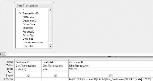
The query shown in Figure 7-1 demonstrates how to use a subquery in the design grid. As you look at this, remember that this is just one example of how a subquery can be used. Subqueries are not limited to use as criteria.
If you were to build the query in Figure 7-1 and switch to SQL view, you would see a SQL statement similar to this one. Can you pick out the subquery? Look for the second SELECT statement.
SELECT CustomerID, Sum(LineTotal) AS SumOfLineTotal
FROM Dim_Transactions
WHERE CustomerID IN
(SELECT [CustomerID] FROM [Dim_Customers] WHERE [State] = "CA")
GROUP BY CustomerID
The idea behind a subquery is that the subquery is executed first, and the results are used in the outer query (the query in which the subquery is embedded) as a criterion, an expression, a parameter, and so on. In the example shown in Figure 7-1, the subquery first returns a list of CustomerIDs for customers in California. Then the outer query uses that list as criteria to filter out any CustomerIDs not in California.
You should know that subqueries often run more slowly than standard queries using joins. This is because subqueries either are executed against an entire dataset or are evaluated multiple times—one time per each row processed by the outer query. This makes them slow to execute, especially if you have a large dataset. So why use them?
Many analyses require multiple step processes that use temporary tables or transitory queries. Although there is nothing inherently wrong with temporary tables and queries, an excess number of them in your analytical processes could lead to a confusing analytical process as well as a database that bloats easily.
Even though using subqueries comes with a performance hit, it may be an acceptable trade for streamlined procedures and optimized analytical processes. You will even find that as you become more comfortable with writing your own SQL statements, you will use subqueries in on-the-fly queries to save time.
There are a few rules and restrictions that you must be aware of when using subqueries.
Your subquery must have, at a minimum, a
SELECTstatement and aFROMclause in its SQL string.You must enclose your subquery in parentheses.
Theoretically, you can nest up to 31 subqueries within a query. This number, however, is based on your system's available memory and the complexity of your subqueries.
You can use a subquery in an expression as long as it returns a single value.
You cannot use the
DISTINCTkeyword in a subquery that includes theGROUP BYclause.
You may have a tendency to shy away from subqueries because you may feel uncomfortable with writing your own SQL statements. Indeed, many of the SQL statements necessary to perform the smallest analysis can seem daunting.
Imagine, for example, that you have been asked to provide the number of account managers that have a time in service greater than the average time in service for all account managers. Sounds like a relatively simple analysis, and it is simple when you use a subquery. But where do you start? Well, you could just write an SQL statement into the SQL view of a query and run it. But the truth is that not many Access users create SQL statements from scratch. The smart ones utilize the built-in functionalities of Access to save time and avoid headaches. The trick is to split the analysis into manageable pieces, as shown in the following steps:
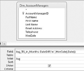
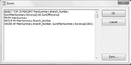
Find the average time in service for all account managers. To do this, create the query shown in Figure 7-2.
Switch to SQL view, shown in Figure 7-3, and copy the SQL statement.
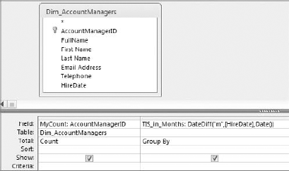
Create a query that will count the number of account managers by time in service. Figure 7-4 does just that.
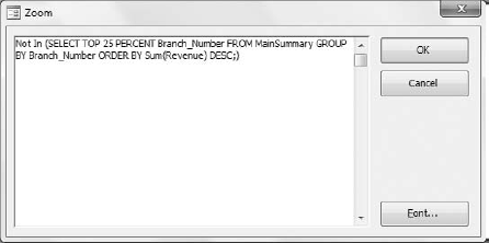
Right-click in the Criteria row under the TIS_in_Months field and select Zoom. This opens the Zoom dialog shown in Figure 7-5. The Zoom dialog does nothing more than help you more comfortably work with text that is too long to be easily seen at one time in the query grid.
With the Zoom dialog box open, paste the SQL statement you copied previously into to the white input area.
Note
Remember that subqueries must be enclosed in parentheses, so you want to enter parentheses around the SQL statement you just pasted. You also need to make sure you delete all carriage returns that were put in automatically by Access.
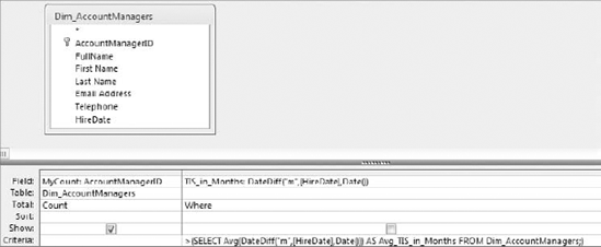
Finish off the query by entering a greater than (
>) sign in from of your subquery and change the aggregate function of the TIS_in_Months row to aWHEREclause. At this point, your query should look like the one shown in Figure 7-6.
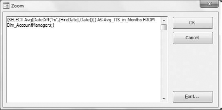
Figure 7.5. Paste the first SQL statement you copied into the Criteria row of the TIS_IN_MONTHS field.
Now if you go to the SQL view of the query shown in Figure 7-6, you will see the following SQL statement:
SELECT Count(AccountManagerID) AS MyCount
FROM Dim_AccountManagers
WHERE (((DateDiff("m",[HireDate],Date()))
>(SELECT Avg(DateDiff("m",[HireDate],Date())) AS Avg_TIS_in_Months
FROM Dim_AccountManagers;)));
The beauty is that you do not have to type all this syntax. You simply use your knowledge of Access to piece together the necessary actions that needed to be taken in order to get to the answer. As you become more familiar with SQL, you will find that you can create subqueries manually with no problems.
The IN and NOT IN operators enable you to run two queries in one. The idea is that the subquery executes first, and then the outer query uses the resulting dataset to filter the final output.
The example demonstrated in Figure 7-7 first runs a subquery that selects all customers based in CA (California). The outer query then uses the resulting dataset as a criteria to return the sum of LineTotal for only those customers that match the customer numbers returned in the subquery.
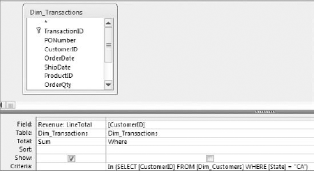
Figure 7.7. This query uses the IN operator with a subquery, allowing you to run two queries in one.
You would use NOT IN to go the opposite way and return the sum of LineTotal for customers that do not match the customer numbers returned in the subquery.
Tip
You can find the query examples in this section in the sample database for this book, located at www.wiley.com.
As its name implies, a comparison operator (=, <, >, <=, >=, <>, and so on) compares two items and returns True or False. When you use a subquery with a comparison operator, you are asking Access to compare the resulting dataset of your outer query to that of the subquery.
For example, to return all customers who have purchases greater than the average purchase for all customers, you can use the following query (Figure 7-8):
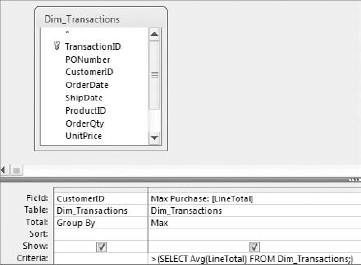
Figure 7.8. Use comparison operators to compare the resulting dataset of your outer query to the results of the subquery.
The subquery runs first, giving you the average purchase for all customers. This is a single value that Access then uses to compare the outer query's resulting dataset. In other words, the max purchase for each customer is compared to the company average. If a customer's maximum purchase is greater than the company average, it is included in the final output; otherwise, it is excluded.
Note
A subquery used with a comparison operator must return a single value.
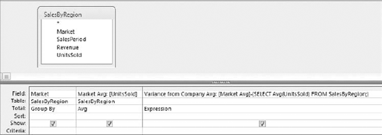
In every example so far, you have used subqueries in conjunction with the WHERE clause, effectively using the results of a subquery as criteria for your outer query. However, you can also use a subquery as an expression, as long as the subquery returns a single value. The query shown in Figure 7-9 demonstrates how you can use a subquery as an expression in a calculation.
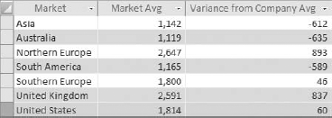
This example uses a subquery to get the average units sold by the entire company; that subquery returns a single value. You are then using that value in a calculation to determine the variance between each market's average units sold and the average for the company. The output of this query is shown in Figure 7-10.
A correlated query is essentially a subquery that refers back to a column that is in the outer query. What makes correlated subqueries unique is that while standard subqueries are evaluated one time to get a result, a correlated subquery has to be evaluated multiple times: once for each row processed by the outer query. To illustrate this point, consider the following two SQL statements.
This SQL statement uses an uncorrelated subquery. How can you tell? The subquery does not reference any column in the outer query. This subquery is evaluated one time to give you the average revenue for the entire dataset.
SELECT MainSummary.Branch_Number,
     (SELECT Avg(Revenue)FROM MainSummary)
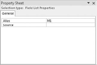
FROM MainSummaryThis SQL statement uses a correlated subquery. The subquery reaches back into the outer query and references the Branch_Number column, effectively forcing the subquery to be evaluated for every row that is processed by the outer query. The result of this query is a dataset that shows the average revenue for every branch in the company. Figure 7-11 demonstrates how this SQL statement looks in Design View.
SELECT MainSummary.Branch_Number,
     (SELECT Avg(Revenue)FROM MainSummary AS M2
     WHERE M2.Branch_Number = MainSummary.Branch_Number) AS AvgByBranch
FROM MainSummary
GROUP BY MainSummary.Branch_NumberThe example shown in Figure 7-9 uses an uncorrelated subquery to determine the variance between each market's average units sold and the average units for the company.
You can apply the same type of technique to correlated subqueries. In the query demonstrated in Figure 7-14, a correlation for each branch number allows you to determine the variance between each employee's annual revenue and the average revenue for that employee's branch.
Action queries can be fitted with subqueries just as easily as select queries can. Here are a few examples of how you would use a subquery in an action query.
This example illustrates how to use a subquery within a make-table query.
SELECT E1.Employee_Number, E1.Last_Name, E1.First_Name
INTO OldSchoolEmployees
FROM Employee_Master as E1
WHERE E1.Employee_Number IN
     (SELECT E2.Employee_Number
     FROM Employee_Master AS E2
WHERE E2.Hire_Date <#1/1/1995#)This example uses a subquery within an append query.
INSERT INTO CustomerMaster (Customer_Number, Customer_Name, State )
SELECT CompanyNumber,CompanyName,State
FROM LeadList
WHERE CompanyNumber Not In
(SELECT Customer_Number FROM CustomerMaster)This example uses a subquery in an update query.
UPDATE PriceMaster SET Price = [Price]*1.1
WHERE Branch_Number In
(SELECT Branch_Number FROM LocationMaster WHERE Region = "South")Domain aggregate functions enable you to extract and aggregate statistical information from an entire dataset (a domain). These functions differ from aggregate queries in that aggregate queries group data before evaluating the values, whereas domain aggregate functions evaluate the values for entire datasets; thus, a domain aggregate function never returns more than one value. To get a clear understanding of the difference between an aggregate query and a domain aggregate function, build the query shown in Figure 7-20.
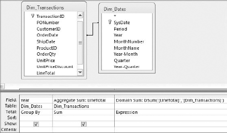
Figure 7.20. This query shows you the difference between an aggregate query and a domain aggregate function.
Run the query to get the results you see in Figure 7-21. You will notice that the Aggregate Sum column contains a different total for each year, whereas the Domain Sum column (the domain aggregate function) contains only one total (for the entire dataset).

Figure 7.21. You can clearly see the difference between an aggregate query and a domain aggregate function.
Note
Although the examples in this chapter show the use of domain aggregate functions in query expressions, keep in mind that you can use these functions in macros, modules, or the calculated controls of forms and reports.
There are 12 different domain aggregate functions in Access, each one performing a different operation. The Table 7-1 lists each function with its purpose and utility.
Table 7.1. Domain Aggregate Functions
Note
DLookup functions are particularly useful when you need to retrieve a value from an outside dataset.
Domain aggregate functions are unique in that the syntax required to make them work varies depending on the scenario. This has produced some very frustrated users who have given up on domain aggregate functions altogether. This section describes some general guidelines that help you in building your domain aggregate functions.
In this example, you are summing the values in the LineTotal field from the Dim_Transactions table (domain). Your field names and dataset names must always be wrapped in quotes.
DSum("[LineTotal]","[Dim_Transactions]")Also, note the use of brackets. Although not always required, it is generally a good practice to use brackets when identifying a field, a table, or a query.
In this example, you are summing the values in the Revenue field from the PvTblFeed table (domain) where the value in the Branch_Number field is 301316. Note that the Branch_Number field is formatted as text. When specifying a criterion that is textual or a string, your criterion must be wrapped in single quotes. In addition, your entire criteria expression must be wrapped in double quotes.
DSum("[Revenue]", "[PvTblFeed]", "[Branch_Number] = '301316' ")Tip
You can use any valid WHERE clause in the criteria expression of your domain aggregate functions. This adds a level of functionality to domain aggregate functions, as they can support the use of multiple columns and logical operators such as AND, OR, NOT, and so on. An example is:
DSum("[Field1]", "[Table]", "[Field2] = 'A' OR [Field2] = 'B'
AND [Field3] = 2")
If you are referencing a control inside of a form or report, the syntax will change a bit.
DSum("[Revenue]", "[PvTblFeed]", "[Branch_Number] =
' " & [MyTextControl] & " ' " )
Notice that you are using single quotes to convert the control's value to a string. In other words, if the value of the form control is 301316, then "[Branch_Number] = ' " & [MyTextControl] & " ' " is essentially translated to read "[Branch_Number] = '301316' ".
In this example, you are summing the values in the LineTotal field from the Dim_Transactions table (domain) where the value in the LineTotal field is greater than 500. Notice that you are not using single quotes, as the LineTotal field is an actual number field.
DSum("[LineTotal]", "[Dim_Transactions]", "[LineTotal] > 500 ")If you are referencing a control inside of a form or report, the syntax changes a bit.
DSum("[LineTotal]", "[Dim_Transactions]", "[LineTotal] >"
[MyNumericControl])
In this example, you are summing the values in the LineTotal field from the Dim_Transactions table (domain) where the value in the OrderDate field is 07/05/2008.
DSum("[LineTotal]", "[Dim_Transactions]", "[OrderDate] = #07/05/08# ")If you are referencing a control inside of a form or report, the syntax changes a bit.
DSum("[LineTotal]", "[Dim_Transactions]", "[OrderDate] =
#" & [MydateControl] & "#")
Notice that you are using number signs to convert the control's value to a date. In other words, if the value of the form control is 07/05/2008, then "[OrderDate] = #" & [MydateControl] & "#" is essentially translated to read "[OrderDate] = #07/05/2008# ".
Like subqueries, domain aggregate functions are not very efficient when it comes to performing large-scale analyses and crunching very large datasets. These functions are better suited for use in specialty analyses with smaller subsets of data. Indeed, you most often find domain aggregate functions in environments where the dataset being evaluated is predictable and controlled (form example, functions, forms, and reports). This is not to say, however, that domain aggregate functions don't have their place in your day-to-day data analysis. This section walks through some examples of how you can use domain aggregate functions to accomplish some common tasks.
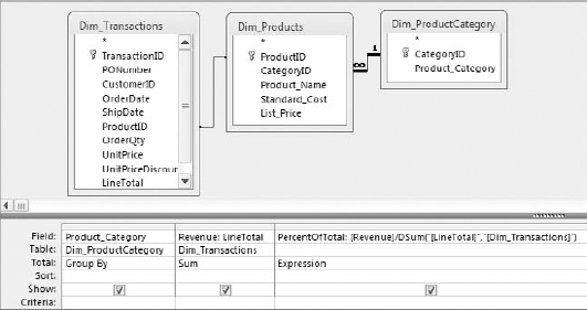
The query shown in Figure 7-22 returns products by group and the sum of LineTotal for each product category. This is a worthwhile analysis, but you can easily enhance it by adding a column that gives you the percent of total revenue for each product.
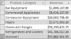
Figure 7.22. You want to add a column that shows the percent of total revenue for each product category.
To get the percent of the total dollar value that each product makes up, you naturally have to know the total dollar value of the entire dataset. This is where a DSum function can come in handy. The following DSum function returns the total value of the dataset:
DSum("[LineTotal]","[Dim_Transactions]")Now you can use this function as an expression in the calculation that returns the "percent of total" for each product group. Figure 7-23 demonstrates how.
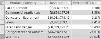
The result, shown in Figure 7-24, proves that this is a quick and easy way to get both total by group and percent of total with one query.
The query in Figure 7-25 uses a DCount function as an expression to return the number of invoices processed on each specific invoice day.
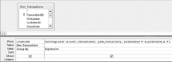
Figure 7.25. This query returns all invoice dates and the number of invoices processed on each date.
Take a moment to analyze what the DCount function is doing.
DCount("[TransactionID]","[Dim_Transactions]","[OrderDate]=
#" & [OrderDate] & "#")
This DCount function retrieves the count of invoices where the invoice date equals (=) each invoice date returned by the query. In the context of the query shown in Figure 7-25, the resulting dataset shows each invoice date and its own count of invoices.
What would happen if you were to alter the DCount function to tell it to return the count of invoices where the invoice date equals or is earlier than (<=) each invoice date returned by the query, as follows?
DCount("[TransactionID]","[Dim_Transactions]","[OrderDate]<=
#" & [OrderDate] & "#")
The DCount function would return the count of invoices for each date and the count of invoices for any earlier date, thereby giving you a running count.
To put this into action, simply replace the = operator in the DCount function with the <= operator, as shown in Figure 7-26.
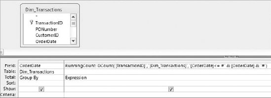
Figure 7.26. Use the <= operator in your DCount function to return the count of invoice dates that equals or is less than the date returned by the query.
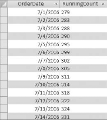
Figure 7-27 shows the resulting running count.
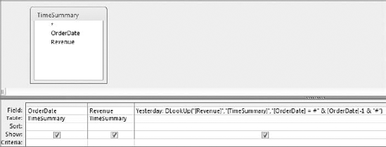
The query in Figure 7-28 uses a DLookup function to return the revenue value from the previous record. This value is placed into a new column called "Yesterday."
This method is similar to the one used when creating a running sum in that it revolves around manipulating a comparison operator in order to change the meaning of the domain aggregate function. In this case, DLookup searches for the revenue value where the invoice date is equal to each invoice date returned by the query minus one (-1). If you subtract one from a date, you get yesterday's date!
DLookUp("[Revenue]","[TimeSummary]","[OrderDate] =
#" & [OrderDate]-1 & "#")
Tip
If you add 1, you get the next record in the sequence. However, this trick does not work with textual fields. This only works with date and numeric fields. If you are working with a table that does not contain any numeric or date fields, create an autonumber field. This gives you a unique numeric identifier that you can use.
Running the query in Figure 7-28 yields the results shown in Figure 7-29.
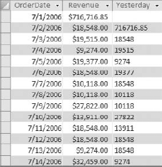
Figure 7.29. You can take this functionality a step further and perform a calculation on the Yesterday field.
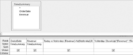
You can enhance this analysis by adding a calculated field that gives you the dollar variance between today and yesterday. Create a new column and enter [Revenue]-NZ([Yesterday],0), as shown in Figure 7-30. Note that the Yesterday field is wrapped in an NZ function in order to avoid errors caused by null fields.
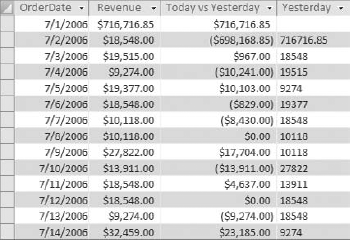
Figure 7-31 shows the result.
Subqueries and domain aggregate functions allow you to build layers into your analysis within one query, eliminating the need for temporary tables or transitory queries. You can leverage both subqueries and domain aggregate functions to streamline your analytical processes, as well as expand and enhance your analysis.
Subqueries are select queries nested within other queries, allowing you to use the results of one query within the execution of another. The idea behind a subquery is that the subquery is executed first, and the results are used in the outer query (the query in which the subquery is embedded) as a criterion, an expression, a parameter, and so on. Although subqueries often run more slowly than standard queries using joins, there are situations where the performance hit may be an acceptable trade for streamlined procedures and optimized analytical processes.
Domain aggregate functions enable you to extract and aggregate statistical information from an entire dataset (a domain). Unlike aggregate queries where the data is grouped before evaluation, domain aggregate functions evaluate the values for the entire dataset. There are 12 different domain aggregate functions: DSum, DAvg, DCount, DLookup, DMin, DMax, DFirst, DLast DStDev, DStDevP, DVar, and DVarP. Domain aggregate functions are ideal for specialty analyses such as calculating the percent of total, creating a running count, creating a running sum, or using values from previous records.

