12
Bench Time: Differential Power Analysis

This lab walks through a complete attack on a bootloader that’s using AES-256 encryption in order to demonstrate how to use side-channel power analysis on practical systems. The AES-256 bootloader in this lab is specifically created for this exercise. The victim microcontroller will receive a command through a serial connection, decrypt the command, and confirm that the included signature is correct. Then, it will save the code into memory only if the signature check succeeded. To make this system more robust against cryptographic attacks, the bootloader will use cipher block chaining (CBC) mode. The goal is to find the secret key and the CBC initialization vector so that we can successfully fake our own firmware. In an actual bootloader, there will be much more functionality, such as reading out fuses, setting up the hardware, and so on, that we don’t implement because it is irrelevant for a side-channel analysis (SCA) attack.
Bootloader Background
In the world of microcontrollers, a bootloader is a specific piece of code that is made to let the user upload new firmware into memory, which is especially useful for devices with complex code that may need to be patched or otherwise updated in the future. The bootloader receives information from a communication line (a USB port, serial port, Ethernet port, Wi-Fi connection, and so on) and stores that data into program memory. Once it has received the full firmware, the microcontroller can happily run its updated code.
Bootloaders have one major security concern. A manufacturer may want to stop arbitrary parties from writing their own firmware and uploading it onto the microcontroller. This could be for protection reasons, as attackers might be able to access parts of the device that weren’t meant to be accessed if they can get early boot access to the microcontroller. Another common reason is to protect a manufacturer’s business interests; in the gaming and printer industries, hardware is sold below manufacturing cost, and that cost is recovered through selling games and cartridges that are locked to a platform. Security features anchored in Secure Boot are used to implement this lock, and bypassing it therefore jeopardizes the business model.
The most common way of stopping execution of arbitrary firmware is to add digital signing (and optionally encryption). The manufacturer can add a signature to the firmware code and encrypt it with a secret key. Then, the bootloader can decrypt the incoming firmware and confirm that it is correctly signed. Users will not know the encryption or signing key tied to the firmware, so they won’t be able to create their own boot code.
In this lab, the bootloader uses a secret AES key to sign and encrypt the firmware. We’ll show you how to extract it.
Bootloader Communications Protocol
For this lab, the bootloader’s communications protocol operates over a serial port at a 38,400 baud rate. The bootloader is always waiting for new data to be sent in this example; in real life, one would typically force the bootloader to enter through a command sequence or a special strap being present during boot (see, for example, the section “The Boot Configuration Pins” in Chapter 3. Figure 12-1 shows what the commands sent to the bootloader look like.

Figure 12-1: The bootloader frame format
The frame in Figure 12-1 has four parts:
- 0x00: One byte of the fixed header.
- Signature: A secret 4-byte constant. The bootloader will confirm that this signature is correct after decrypting the frame.
- Data: Twelve bytes of the incoming firmware. This system forces us to send the code 12 bytes at a time; more complete bootloaders may allow longer, variable-length frames. The bytes are encrypted using AES-256 in CBC mode (described in the next section).
- CRC-16: A 16-bit checksum using the CRC-CCITT polynomial (0x1021). The least significant bit (LSB) of the cyclic redundancy check (CRC) is sent first, followed by the most significant bit (MSB). The bootloader will reply over the serial port, describing whether or not this cyclic redundancy check was valid.
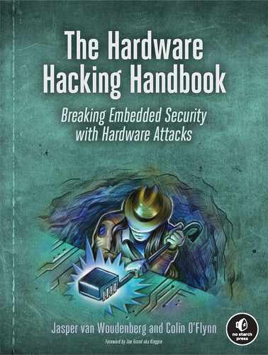
The bootloader responds to each command with a single byte indicating whether the CRC-16 was okay (see Figure 12-2).
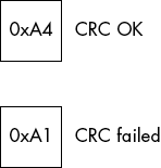
Figure 12-2: The bootloader response format
After replying to the command, the bootloader verifies that the signature is correct. If it matches the expected manufacturer’s signature, the 12 bytes of data will be written to flash memory. Otherwise, the data is discarded. The bootloader provides no indication to the user of whether the signature check passed.
Details of AES-256 CBC
The system uses the AES-256 block cipher in cipher block chaining (CBC) mode. In general, one avoids using encryption primitives as is (that is, Electronic Code Book, or ECB) since it means the same piece of plaintext always maps to the same piece of ciphertext. Cipher block chaining ensures that if you encrypted the same sequence of 16 bytes a bunch of times, the encrypted blocks are all different.
Figure 12-3 shows how AES-256 CBC decryption works. The details of the AES-256 decryption block will be discussed in detail later.

Figure 12-3: Decryption using AES-256 with cipher block chaining: the ciphertext of one block is used in the decryption of the next block, which results in a chain of dependencies on previous ciphertext blocks.
Figure 12-3 shows that the output of the decryption is not used directly as the plaintext. Instead, the output is XORed with a 16-byte value, which is taken from the previous ciphertext. Since the first decryption block has no previous ciphertext to use, an initialization vector (IV) is used instead. For cryptographic security, the IV is usually considered public, but in our example, we’ve kept it secret to show how to recover it if it is not available. If we are going to decrypt the entire ciphertext (including block 0) or correctly generate our own ciphertext, we’ll need to find this IV along with the AES key.
Attacking AES-256
The bootloader in this lab uses AES-256 decryption, which has a 256-bit (32-byte) key, and this means our regular AES-128 CPA attacks won’t work out of the box; we’ll need a few extra steps. First, we perform a “regular” AES-128 CPA attack on the inverse S-box output to get the round 14 key. We target the inverse S-box because it’s a decryption, and the first round of decryption has number 14. Using the found round key, we can calculate the inputs to round 13. Next, we’ll use “one special trick” (described next) to perform CPA on the round 13 inverse S-box output to get a “transformed” round 13 key. Once we have that, we transform this round key into the regular round 13 key. Now we have two round keys, which is sufficient to use the inverse key schedule to recover the full AES-256 key. The magic is in the transformed keys, so let’s dig into those.
First, we assume that we’ve recovered the round 14 key using regular CPA. This allows us to calculate the output of round 14. For an AES decryption, this round 14 output is input to round 13, so we’ll call it X13. We cannot simply do the same CPA attack on round 13 as on round 14 because of the presence of the inverse MixColumns operation (MixColumns–1) in the round 13. The MixColumns–1 operation takes 4 bytes of input and generates 4 bytes of output. Any change in a single byte will result in a change of all 4 bytes of output. We need to perform a guess over 4 bytes instead of 1 byte, which would mean we have to iterate over 232 guesses instead of 28. This would be a considerably more time-consuming operation.
To solve this, we’ll do a little bit of algebra, starting by writing round 13 as an equation. The state at the end of round X13 is a function of the input to round X14 and the round key K13:
X13 = SubBytes–1(ShiftRows–1(MixColumns–1(X14 ⊕ K13)))
MixColumns–1 is a linear function; that is:
MixColumns–1(A ⊕ B) = MixColumns–1(A) ⊕ MixColumns–1(B)
The same holds for ShiftRows–1. We can rewrite the equation for X13 by using this fact:
X13 = SubBytes–1(ShiftRows–1(MixColumns–1(X14)) ⊕ ShiftRows–1(MixColumns–1(K13)))
We’ll introduce K'13, the transformed key for round 13:
K'13 = ShiftRows–1(MixColumns–1(K13)))
And we can use this transformed key to state the output X13 as follows:
X13 = SubBytes–1(ShiftRows–1(MixColumns–1(X14)) ⊕ K'13)
Using this equation, you see that K'13 is just a vector of bits we can recover using CPA, without a dependency on MixColumns–1. Therefore, we can perform a CPA attack on the individual bytes of output of SubBytes–1 to recover each transformed subkey one byte at a time. Once we have a best guess for all transformed subkey bytes, we can recover the actual round key by reversing the transformation:
K13 = MixColumns(ShiftRows(K'13)))
The final step is trivial: using the inverse AES-256 key schedule, we can use the K13 and K14 keys to determine the full AES-256 encryption key. Don’t worry if you’re not fully able to follow this; the Jupyter notebook companion to this chapter (https://nostarch.com/hardwarehacking/) has the necessary code.
Obtaining and Building the Bootloader Code
Follow the instructions at the top of the companion notebook for this chapter to get set up, specifically setting SCOPETYPE correctly. If you are just following along with traces, they are provided in the virtual machine (VM). We recommend you first follow along using the provided pre-captured traces. The companion Jupyter notebook contains all the code to run the analysis, including all the “answers.” To avoid giving everything away directly, we’ve encrypted the answers with military-grade RSA-16. Try to find these answers yourself first.
If you are using the ChipWhisperer hardware as a target, use this notebook to compile the bootloader and load it to the target by running all the cells in the notebook section corresponding to this section. Make sure you can see the flash is programmed and verified.
If you aren’t using the ChipWhisperer as a target, you’ll need to port, compile, and load the bootloader code yourself. The top of the notebook has a link to the code. For porting, check the main() function in bootloader.c for the platform_init(), init_uart(), trigger_setup(), trigger_high(), and trigger_low() calls. The simpleserial library is included, and it uses putch() and getch() to communicate with the serial console. You can see the various hardware abstraction layers (HALs) in the victims/firmware/hal folder. The most basic HAL that you can use as a reference is the ATmega328P HAL in the victims/firwmare/hal/avr folder. If one of the HALs already matches the device you want to run on, it is sufficient to specify PLATFORM=YYY in the notebook with the matching platform YYY based on the HAL folder. Make sure you have firmware built and flashed before proceeding.
Running the Target and Capturing Traces
Let’s get some traces. If you’re running without hardware, this step can be skipped. With hardware, you’ll need to set up the target and send it messages it will accept, so you’ll need to deal with serial communication and calculating that CRC.
If you have access to a ChipWhisperer, try this on ChipWhisperer-Lite XMEGA (“classic”) or ChipWhisperer-Lite Arm platforms. Alternatively, you can follow with your own SCA setup and/or target. We discussed how to set up your own power measurement in Chapter 9; the physical measurements for simple power analysis and correlation power analysis are identical, so refer to that chapter for more details of the setup procedure with your own equipment. The bootloader code we use in this chapter will also run on the ATmega328P, so if you used the Arduino Uno–based power capture setup, you can almost directly run the bootloader code.
In this lab, we have the luxury of seeing the bootloader’s source code, which is generally not something we’d have access to in the real world. We’ll run the lab as if we don’t have that knowledge and later have a look to confirm our assumptions.
Calculating the CRC
If you are running on a physical target, the next step in attacking this target is to communicate with it. Most of the transmission is fairly straightforward, but the CRC is a little tricky. Luckily, there’s a lot of open source code out there for calculating CRCs. In this case, we’ll import some code from pycrc, which can be found on our notebook. We initialize it with the following line of code:
bl_crc = Crc(width = 16, poly=0x1021)Now we can easily get the CRC for our message by calling
bl_crc.bit_by_bit(message)This means our message will pass the basic acceptability test by the bootloader. In real life, you may not know the CRC polynomial, which was the value we passed with the poly parameter in initializing the CRC. Luckily, bootloaders often use one of only several common polynomials. The CRC is not a cryptographic function, so the polynomial is not considered a secret.
Communicating with the Bootloader
With that done, we can start communicating with the bootloader. Recall that the bootloader expects blocks to be formatted as in Figure 12-1, which includes a 16-byte encrypted message. We don’t really care what the 16-byte message is, just that each is different so that we get a variety of Hamming weights for our upcoming CPA attack. We’ll therefore use the ChipWhisperer code to generate random messages.
We can now run the target_sync() function in order to sync with the target. This function should get 0xA1 from the target, meaning the CRC failed. If we don’t get 0xA1 back, we loop until we do. At that point, we’re synchronized with the target. Next, we’ll send a buffer with a correct CRC in order to check that our communication is working properly. We send a random message with a correct CRC, and we should receive 0xA4 as the response.
When we see this response, we know our communication has worked as intended, and we can move on. Otherwise, it’s time to debug. A typical issue is wrong communications parameters (38,400 baud, 8N1, no flow control). Try to connect manually using a serial terminal to the target and press enter until you start seeing responses. Also, a failing serial connection can be debugged using a logic analyzer or oscilloscope. Check that you are seeing line toggles and that they are at the right voltage and baud. If you are seeing no response, it could be the target device isn’t starting up (does it require a clock signal and is one provided?), or you are not connecting to the correct TX/RX pairs.
Capturing Overview Traces
With that out of the way, we can proceed to capturing our traces. Since this is AES implemented in software on a microcontroller, we can visually identify the AES execution by spotting the 14 rounds. We’re performing AES-256 decryption, so round 14 is the first round that is executed!
We’ll take a first capture with the following settings:
- Sampling rate: 7.37 MS/s (mega-samples per second, 1× device clock)
- Number of samples: 24,400
- Trigger: Rising edge
- Number of traces: Three
For the initial capture, we just want to get an overview of the operations happening on the chip, which means for the number of samples, it’s fine to take some really high number that you know for sure can capture the entire operation of interest. Ideally, you want to see the end of the operations clearly. The end is typically characterized by some infinite loop, where the device is waiting for more input, so that is visible at the tail end of a trace as an infinitely repeating pattern. Figure 12-4 shows the overview trace for the XMEGA target, which is cropped only to the AES-256 operation.

Figure 12-4: Power trace of AES-256 execution on the ChipWhisperer XMEGA target
We actually don’t see the end of the operation, but in this case, we’re interested only in the beginning rounds. By zooming in, we can identify that the first two rounds of the decryption are happening within the first 4,000 samples, allowing us to narrow down the number of samples in our follow-up capture.
If your overview trace doesn’t show the AES clearly, consider all connections and configurations of your target and scope and then try to isolate the problem:
- Check that the target correctly outputs the trigger and that the scope responds to the trigger. You can capture the trigger on the scope to debug this.
- Check the signal channel. You’ll need to see some activity on this, even if you don’t recognize the AES in it.
- Check the cables and configuration.
It’s also possible that your target simply doesn’t leak so much (for instance, if you’re using hardware-accelerated crypto). You can then start pinpointing crypto by using correlation analysis or a t-test, as described in Chapters 10 and 11, respectively. For the purpose of this lab, that is out of scope.
Capturing Detailed Traces
Assuming you have an overview trace and have identified the first two rounds, use the following settings and rerun the preceding loop to capture a batch of data:
- Sampling rate: 29.49 MS/s (4× device clock)
- Number of samples: 24,400
- Trigger: rising edge
- Number of traces: 200
The number 200 is an initial guess: software AES on a microcontroller typically leaks like a sieve, so you don’t need many traces. If during analysis you are unable to find any leakage, you may have to increase this number and retry. To give you another data point: any seriously protected implementation, or crypto running on a System-on-Chip (SoC) can require easily millions (and up to tens of millions) of traces to find any leakage.
Analysis
Now that you have power traces, you can perform the CPA attack. As described previously, you’ll need to do two attacks: one to get the round 14 key and another (using the first result) to get the round 13 key. Finally, you’ll do some post-processing to get the 256-bit encryption key.
Round 14 Key
We can attack the round 14 key with a standard, no-frills CPA attack (using the inverse S-box, since it’s a decryption that we’re breaking). Python chews through 24,400 samples rather slowly, so if you want a faster attack, use a smaller range. If you count the rounds in Figure 12-4, you can narrow down the range of samples to only round 14. The sampling frequency in the detailed traces is four times higher than the overview, so make sure to account for that.
When running the analysis code on the pre-acquired traces, we get the table shown in Figure 12-5 as a result. This table contains the key you’re looking for, so peep at it only if you want the answers.

Figure 12-5: The top five candidates and their correlation peak height for each of the 16 subkeys for the round 14 key
The columns in this table show the 16 subkey bytes. The five rows are the five highest-ranking subkey hypotheses, ranked by decreasing (absolute) correlation peak height. The numbers will vary if you run this on hardware; although if all is well, you will get the same key bytes at rank 0. From this table, we can make a few observations. Since this table represents only 128 bits of the full AES-256 key, we cannot use a ciphertext/plaintext pair to verify that this part of the key is correct. In fact, because we don’t have decrypted firmware, we don’t even know the plaintext, so we can’t do that test in the first place.
We could just hope we got this half of the key right and move on. However, if we have one bit wrong in the key for round 14, we will get completely stuck when trying to recover the key for round 13. This is because we’ll need to calculate the inputs for round 13, which relies on a correct round 14 key. If the inputs are calculated incorrectly, we won’t be able to find any correct correlations for CPA.
To gain some confidence that this is indeed the correct key, we look at the correlation values between the different candidates per subkey. For instance, for subkey 0, the correlations for the top five candidates are 0.603, 0.381, 0.339, 0.332, and 0.312. The top candidate’s correlation is much higher than the others, meaning we have a high confidence that 0xEA is the right guess. If the top candidate’s correlation were 0.385, that would give us much lower confidence as it is much closer to the other candidates.
As the table in Figure 12-5 shows, for every subkey, the top candidate has a much higher correlation than the second, so we’re confident enough that we can move on. As a rule of thumb, if for every subkey the difference between the top candidate and the second candidate is an order of magnitude larger than the difference between the second candidate and the third candidate, it’s generally safe to move on.
If you are following along with your own measurements, do that check. If your correlations show poor confidence, either try to take more traces or work on better processing of the traces, which could include any of the techniques described in Chapter 11, such as filtering, alignment, compression, and resynchronization. Also, don’t despair! It’s extremely rare to get proper leakage on a first try, and this is your opportunity to put some real processing and analysis to work.
Next, the notebook gathers the key bytes in the rec_key variable and prints out the correlation values. It’ll also tell you whether you got the key correct! Let’s move on to the next half of the key.
Round 13 Key
For round 13, we’ll need to deal with some misalignment in the XMEGA traces, and we’ll need to add a leakage model using the “transformed” key.
Resyncing Traces
If you’re following along on the XMEGA version of the firmware, the traces become desynced before the leakage in round 13 occurs. Figure 12-6 shows the desynchronized traces. The desynchronization is due to a nonconstant time AES implementation; the code does not always take the same amount of time to run for every input. (It’s actually possible to do a timing attack on this AES implementation. We’ll stay on topic with our CPA attack, though.)
While this does open up a timing attack, it actually makes our AES attack a little harder, since we’ll have to resync (resynchronize) the traces. Luckily, we can do that pretty easily using the ResyncSAD preprocessing module. It takes in a reference pattern (ref_trace and target_window) and matches that to other traces using the sum of absolute differences (explained in the “Resynchronization” section in Chapter 11) to find how much to shift the other traces for alignment. When we apply this module, the traces are aligned around the target window. The bottom graph of Figure 12-6 shows the result.

Figure 12-6: Desynchronized traces on top, and resynchronized traces on the bottom
Leakage Model
The ChipWhisperer code doesn’t have a leakage model for the round 13 key built in, so we’ll need to create our own. The leakage() method in the notebook takes in the 16 bytes of input to the AES-256 decryption in the pt parameter, which it then runs through round 14 of decryption using the previously found round 14 key (in k14), followed by a ShiftRows–1 and a SubBytes–1, which produces x14.
Next, it runs x14 through a partial round 13 decrypt with the transformed key we explained earlier:
X13 = SubBytes–1(ShiftRows–1(MixColumns–1(X14)) ⊕ K'13)
So, we take x14 and run it through MixColumns-1 and ShiftRows–1. Then we XOR in a single byte key guess of the transformed key K'13 (guess[bnum]), and finally we apply an individual S-box. The output X13 is the intermediate value we return for the CPA leakage modeling.
Running the Attack
Like in the round 14 attack, we can use a smaller range of points to make the attack faster. After running this attack, we get the table of results shown in Figure 12-7.
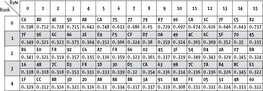
Figure 12-7: The top five candidates and their correlation peak height for each of the 16 subkeys for the transformed round 13 key
The correlations look good for each of the first candidates: the correlation peaks for the candidates ranked 0 are sufficiently higher than for the candidates ranked 1. If they do in your case as well, you can move on.
If it doesn’t look good on your end, check all your parameters (twice), check that the first found key actually had good correlations, and check the alignment for this round. If that doesn’t solve the problem, it’s a mystery indeed; normally the different rounds of AES require the same preprocessing (except for alignment), so it’s odd to reach this point being able to extract the key for round 14 fully and not 13. All we can recommend is to review every step carefully and use a known key correlation or t-test (see the “Test Vector Leakage Assessment” section in Chapter 11) to figure out whether you can find the key when you know the key. As mentioned before, keep chipping away at it.
When you do have the transformed round 13 key, run the block in the notebook so that this key is printed out and recorded in rec_key2. To get the real round 13 key, the notebook runs what you’ve recovered through a ShiftRows and MixColumns operation. Next, it combines the round 13 and 14 keys and then calculates the full AES key by running the AES key schedule appropriately.
You should see the 32-byte key printed out. Celebrate if it’s correct! If not, check your code with the keys we’ve provided to make sure it works properly.
Recovering the IV
Now that we have the encryption key, we can proceed onto an attack of the next secret value: the initialization vector (IV). Often cryptographic IVs are considered public information and are thus available, but the author of this bootloader decided to hide it. We’ll try to recover the IV using a differential power analysis (DPA) attack, which means we’ll need to capture traces of some operation that combines known, varying data with the unknown, constant IV. Figure 12-3 shows that the IV is combined with the output coming out of the AES-256 decrypt block. Since we have recovered the AES key, we know and control this output. That means we have all the ingredients to target the XOR operation that combines the output with the IV using DPA.
What to Capture
The first question to ask is, “When could the microcontroller actually perform the XOR operation?” In this case, “could” refers to hard limits; for instance, we can do the XOR only after all of the inputs to the XOR are known, so we know the XOR will never happen before the first AES decrypt. The XOR will also happen at least before the plaintext firmware is written to flash. If we can find the AES decrypt and the flash write in the power trace, we are certain the XOR will be somewhere in between.
However, often this still leads to a rather large window, so the next question is, “When would the microcontroller actually perform the XOR operation?” In this case, “would” refers to sanity on the developer side. The code will probably apply the XOR soon after the AES decrypt has completed, though that is not a solid guarantee. The developer could have made other choices. Often the developer does something sane, so with a bit of rationalization, you can shrink the acquisition window. If you shrink the window to be too small, you might cut out the operation altogether, which will mean your attack fails. The reason we try to perform such optimization, even with the risk of total failure, is that the smaller window will give us smaller files, meaning a faster attack and ability to capture more traces. In addition, the actual attack will almost always perform better with a smaller window, as a smaller window means you are cutting out unnecessary noise—the noise will ultimately degrade the attack performance.
Going forward, let’s use the completion of the AES-256 as a starting point for our capture of the IV XOR. Recall that the trigger pin is pulled low after the decryption finishes. This means we can start acquisition after the AES-256 function by triggering our scope on a falling edge of the trigger.
The question now is how many samples to capture, which will be a bit of informed guesswork. From our previous capture, we know a 14-round AES fits within 15,000 samples. So, a simple XOR of 16 bytes should be significantly shorter, at least less than one round (say 1,000 samples). However, we don’t know how soon after the AES the XOR is calculated. Just to be safe, we settle on 24,400 samples for the single trace overview.
Getting the First Trace
Now that we have a guess at what to acquire, let’s have a look at the acquisition code. There are a few additional aspects to consider now compared to the acquisition of the AES operation:
- The IV is applied only on the first decryption, which means we’ll need to reset the target before each trace we capture.
- We trigger on the falling edge to capture operations after the AES.
- Depending on the target, we may have to flush the target’s serial lines by sending it a bunch of invalid data and looking for a bad CRC return. This step slows down the capture process significantly, so you may want to try without doing this first.
The notebook code implements the required capture logic, and if the capture is successful, it plots a single trace for us to inspect (see Figure 12-8). The acquisition parameters are as follows:
- Sampling rate: 29.49 MS/s (4× device clock)
- Number of samples: 24,400
- Trigger: Falling edge
- Number of traces: Three
Try to find the range in which you think the IV is calculated before moving on. Think about the order and duration of operations of what could happen after the AES calculation in an AES CBC.
Now, we must make an educated guess as to whether this is a good enough window of the operations to continue. It seems that between 0 and about 1,000 samples there are 16 repetitions, and also between 1,000 and 2,000. Their duration (number of samples) aligns with our expectation of about 1,000 samples. We’ll continue with the assumption that between 0 and 1,000, somewhere the XOR is happening. If we don’t end up finding an IV, we may have to reconsider this assumption.
If you’re not seeing a nice overview trace on your own acquisition, jump back to the “Capturing Overview Traces” section in this chapter for details on getting an overview trace for AES. Sometimes it can be helpful to jump back a few steps if you lose the signal.

Figure 12-8: Power trace just after the AES operation, with the IV XOR hiding somewhere
Getting the Rest of the Traces
Now that we have a proper idea of when the XOR is happening from our overview trace, we can move on to our capture. It’s pretty similar to the last one, except you’ll notice the acquisition will be a lot slower. This is because we must reset the target between each of the captures in order to reset the device to the initial IV.
Now, we’ll store our traces in Python lists and we’ll convert to NumPy arrays later for easy analysis. As for the number of traces, N, let’s take about the same amount as we did for the AES, since the leakage characteristics are probably similar.
You can visually inspect a few captured traces to confirm that they look the same as the overview trace, and then you’re ready to analyze. If they look different, go back and see what changed between capturing the overview trace and these traces.
Analysis
Now that we have a batch of traces, we can perform a classical DPA attack to recover individual bits of the IV. Attacking an XOR is typically harder than attacking crypto because of crypto’s diffusion and confusion properties: any nonlinearity helps correlation as a distinguisher. For instance, in AES, if we guess one bit of a key byte wrong, half of the output bits of an S-box will be guessed incorrectly, and correlation with the traces will drop significantly. For the XOR “key,” the IV, if we guess one key bit wrong, only one bit of the XOR output will be wrong, so correlation with traces drops less significantly. Because we’re attacking a software implementation, we’ll probably be okay because it will have high leakage. However, when the XOR is implemented in hardware, it could take hundreds of millions to billions of traces to get correlation. At that point, you may want to graduate out of Python scripts.
Attack Theory
The bootloader applies the IV to the AES decryption result by performing an XOR, which we’ll write as
PT = DR ⊕ IV
Here, DR is the decrypted ciphertext, IV is the secret initial vector, and PT is the plaintext that the bootloader will use later, each 128 bits. Since we know the AES-256 key, we can calculate DR.
This is enough information for us to attack a single bit of IV by calculating the difference of means: the classical DPA attack (see Chapter 10). Let’s say DRi is the ith bit of DR, and suppose we wanted to get the ith bit IVi. We could do the following:
- Split all of the traces into two groups: those with DRi = 0, and those with DRi = 1.
- Calculate the average trace for both groups.
- Find the difference of means (DoM) for both groups. It should include noticeable spikes, corresponding to all usages of DRi.
- If the direction of the spikes is the same, the IVi bit is 0 (PTi == DRi). If the direction of the spike flips, the IVi bit is 1 (PTi == ~ DRi).
We can repeat this attack 128 times to recover the entire IV.
Doing the One-Bit Attack
Let’s have a look at the direction and location of the spikes, which we’ll have to pinpoint if we want to grab all 128 bits. To keep things simple for now, we’ll only focus on the LSB of each byte of the IV. Per the attack theory, we calculate DR using an AES decrypt, and we calculate the DoM for the LSB of each byte. Finally, we plot these 16 DoMs to see if we can spot the positive and negatives spikes (see Figure 12-9).
Figure 12-9: DPA attack on one bit of each byte of the IV
You should see a few visible positive and negative spikes, but it’s hard to conclude which ones are part of the XOR operation and which ones are “ghost peaks.” Since we’re measuring on an 8-bit microcontroller, the XOR is done with 8 bits in parallel, and there is some for loop around the XOR that runs over all 16 bytes, so we’d expect the peaks for each byte to be equally spaced. We can see this somewhat in Figure 12-9, but we have to do a little more work to automate the extraction of all 128 bits.
We’ll make a scatterplot that allows us to find at what point in time each IV byte leaks. We’ll set it up as follows:
- Each mark in the plot represents a leakage location.
- The x-coordinate represents the byte that leaks.
- The y-coordinate represents the location of the leakage in time.
- Each mark has a shape—a star being a positive peak and a circle being a negative peak. This shape therefore indicates whether the IV bit is a 1 or a 0.
- Each mark has a size representing the size of the peak.
- For each x-coordinate, there are a number of marks, representing the highest peaks for that byte.
Because we assume the IV is XORed in a loop, 8 bits at a time, there will be a linear relation between the x- and y-coordinates. Once we have that relation, we can use it to extract the correct peaks in order to get the bit. Figure 12-10 shows the result.
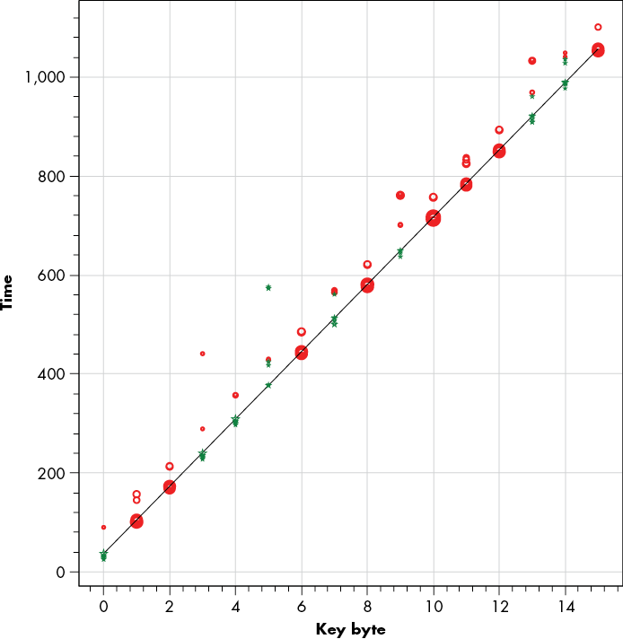
Figure 12-10: Scatterplot showing DPA peaks, allowing us to find the linear relation between bytes and locations in the trace
You may notice there are two reasonable ways of plotting a line through the points. We choose the one where the amplitudes of the peaks are the highest. If this turns out to be wrong, we can try the second line, which is slightly above the black line in Figure 12-10.
Our goal is to extract all IV bits, and we can exploit the regularity of the timing of the XOR operation to create a script to do so.
The Other 127
Now we can attack the entire IV by repeating the 1-bit conceptual attack for each of the bits. The full code is in the notebook, but first try to do this yourself. If you’re stuck, here are a few hints to get you going.
One easy way of looping through the bits is by using two nested loops, like this:
for byte in range(16):
    for bit in range(8):
        # Attack bit number (byte*8 + bit)
The sample to look at will depend on which byte you’re attacking. Remember, all 8 bits in a byte are processed in parallel and will be at the same location in the trace. We had success when we used location = start + byte*slope for the right values of start and slope.
The bit-shift operator and the bitwise-AND operator are useful for getting at a single bit:
#This will either result in a 0 or a 1
checkIfBitSet = (byteToCheck >> bit) & 0x01
Check whether your IV matches the one we have here. If not, first run this script again with the flip variable set to 1. Depending on your target and how you’ve connected it to your scope, the polarity of the peaks may be reversed. You can easily check this by flipping all the found IV bits and trying again.
Attacking the Signature
The last thing we can do with this bootloader is attack the signature. This section shows how you can recover all 4 secret bytes of the signature with an SPA attack. A possible alternative is to use the key to decrypt a single sniffed packet during a firmware load, but that doesn’t involve power measurements, so it doesn’t fit well here.
Attack Theory
One subtle difference you may have spotted when taking traces for the XOR is that in one out of about 256 traces, the operations after the XOR take slightly longer. This effect is probably because the signature comparison has an early termination condition: if the first byte is incorrect, the rest of the bytes aren’t checked. We’ve studied this timing leak effect before in Chapter 8, and we’ll use it here to recover secret information.
To make sure we indeed are observing a timing leak, we can verify it by sending 256 communication packets, each time keeping the ciphertext constant but by varying the first byte of signature to all values from 0 to 255. We’ll observe that exactly one of the packets generates a longer trace, meaning we “guessed” the signature byte correctly. We can then iterate this for the other 3 bytes to create a signature for a packet. Let’s go ahead and verify that our hypothesis is correct (while guessing signatures).
Power Traces
Our capture will be pretty similar to the one we used to break the IV, but now that we know the secret values of the encryption process, we can make some improvements by encrypting the text that we send. This has two important advantages:
- We can control each byte of the decrypted signature (as mentioned earlier, the signature is sent encrypted together with the plaintext), which allows us to hit each possible value once. It also simplifies the analysis, since we don’t have to worry about decrypting the text we sent.
- We need to reset the target only once. We know the IV, and because we know key and plaintext, we can correctly produce the entire CBC chain, which speeds up the capture process considerably.
We’ll run our loop 256 times (one for each possible byte value) and assign that value to the byte we want to check. The next_sig_byte() function in the notebook implements this. We’re not quite sure where the check is happening, so we’ll be safe and capture 24,000 samples. Everything else should look familiar from earlier parts of the lab.
Analysis
After we’ve captured our traces, the actual analysis is pretty simple. We’re looking for a single trace that looks very different from the 255 others. A simple way to find this is to compare all the traces to a reference trace. We’ll use the average of all the traces as our reference. Let’s start by plotting the traces that differ the most from the reference trace. Depending on your target, you might see something like the graph in Figure 12-11.
It looks like there is a trace that is significantly different from the mean, as it creates a huge “band” behind the other traces! However, let’s do this the statistics way. In guess_signature(), we use the correlation coefficient: the closer to 0 the correlation value between the reference trace and the trace-to-test is, the more it deviates from the mean. We want to take the correlation only across where the plots differ, so we choose sign_range, a subset of the plot, where there’s a large difference.
Next, we calculate and print the correlation for the top five traces with the reference:
Correlation values: [0.55993054 0.998865 0.99907424 0.99908035 0.9990855 4]
Signature byte guess: [0 250 139 134 229]
Figure 12-11: The difference between the traces and the reference; one trace significantly differs.
In terms of correlation, one trace is totally different, with much lower correlation (correlation ~0.560, whereas the rest has ~0.999). Because this number is so much lower, it’s probably our correct guess. The second list gives the signature guess that matches each of the preceding correlations. The first number is therefore our best guess of the correct signature byte (in this case, 0).
All Four Bytes
Now that we have an algorithm that works to recover a single byte of the IV, we just need to loop it for all 4 bytes. Basically, we’re using the target as an oracle to guess the correct signature in the worst case (4 × 256 = 1,024 traces) and in the average case (512 traces). The notebook implements this loop and is able to extract the secret signature.
All in all, we’re now able to forge code that the bootloader will accept, and we’re also able to decrypt any existing code by using various power analysis attacks.
Peeping at the Bootloader Source Code
Just for fun, let’s have a look at the code to see whether we can make sense of the traces we found. The bootloader’s main loop does several interesting tasks, as shown in the snippet from bootloader.c, re-created in Listing 12-1. The full bootloader code can be found from the link at the top of the notebook.
  // Continue with decryption
  trigger_high();
  aes256_decrypt_ecb(&ctx, tmp32);
  trigger_low();

  // Apply IV (first 16 bytes)
1 for (i = 0; i < 16; i++){
      tmp32[i] ^= iv[i];
  }

  // Save IV for next time from original ciphertext
2 for (i = 0; i < 16; i++){
      iv[i] = tmp32[i+16];
  }

  // Tell the user that the CRC check was okay
3 putch(COMM_OK);
  putch(COMM_OK);

  // Check the signature
4 if ((tmp32[0] == SIGNATURE1) &&
     (tmp32[1] == SIGNATURE2) &&
     (tmp32[2] == SIGNATURE3) &&
     (tmp32[3] == SIGNATURE4)){

     // Delay to emulate a write to flash memory
     _delay_ms(1);
  }
Listing 12-1: Part of bootloader.c showing the decryption and processing of data
This gives us a pretty good idea of how the microcontroller is going to do its job. The following will use the C file from Listing 12-1.
After the decryption process, the bootloader executes a few distinct pieces of code:
- To apply the IV, it uses an XOR operation applied in a loop 1.
- To store the IV for the next block, it copies the previous ciphertext into the IV array 2.
- It sends 2 bytes on the serial port 3.
- It checks the bytes of the signature, one by one 4.
We should be able to recognize these parts of the code in the power trace. For example, the power trace of the bootloader running on the XMEGA is given in Figure 12-12.
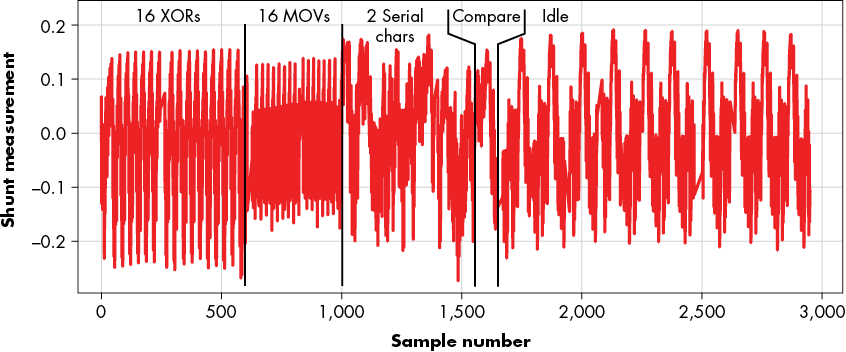
Figure 12-12: A visual inspection of the power trace, with known instructions (based on our knowledge of the code) annotated
The approach to annotating a trace like Figure 12-12 is first to recognize the final “idle” pattern. We can use a trigger to confirm this or just measure a device without sending a command. Then, we can work backward against known operations to build up the annotation. It helps to have an insight into the main loops in the code, because those you can often count in the power trace. These insights can come from code or even just from a hypothesis on what the code should look like, given that it implements some public specification. In this case, we cheated and just used the code.
The location of the peaks we found before aligns in sample numbers with where we are claiming the XOR operations are occurring based on the annotation of the power trace. This suggests we have correctly annotated the power trace.
Timing of Signature Check
The signature check in C looks like this:
if ((tmp32[0] == SIGNATURE1) &&
    (tmp32[1] == SIGNATURE2) &&
    (tmp32[2] == SIGNATURE3) &&
    (tmp32[3] == SIGNATURE4)){
In C, a compiler is allowed to short-circuit calculations of Boolean expressions. When checking multiple conditions, the program will stop evaluating those conditions as soon as it can tell what the final value will be. In this case, unless all four of the equality checks are true, the result will be false. Thus, as soon as the program finds a single false condition, it can stop evaluation of the other conditions.
To look at how the compiler did this, we have to go to the assembly file. Open the .lss file for the binary that was built, available in the same folder as the bootloader code. This is called a listing file, and it lets you see the assembly that the C source was compiled and linked to. Since assembly gives you an exact view of the instructions executed, it can give you a better correspondence to the traces.
Next, find the signature check and confirm that the compiler is using the short-circuit logic (which enables our timing attack). You can confirm this as follows. Let’s take an example of the STM32F3 chip, where the assembly result in the listing file is shown in Listing 12-2.
               //Check the signature
               if ((tmp32[0] == SIGNATURE1) &&
   8000338:   f89d 3018   ldrb.w  r3, [sp, #24]
   800033c:   2b00        cmp r3, #0
   800033e:   d1c2        bne.n   80002c6 <main+0x52>
   8000340:   f89d 2019   ldrb.w  r2, [sp, #25]
 1 8000344:   2aeb        cmp r2, #235    ; 0xeb
 2 8000346:   d1be        bne.n   80002c6 <main+0x52>
                   (tmp32[1] == SIGNATURE2) &&
   8000348:   f89d 201a   ldrb.w  r2, [sp, #26]
 3 800034c:   2a02        cmp r2, #2
 4 800034e:   d1ba        bne.n   80002c6 <main+0x52>
                   (tmp32[2] == SIGNATURE3) &&
   8000350:   f89d 201b   ldrb.w  r2, [sp, #27]
   8000354:   2a1d        cmp r2, #29
   8000356:   d1b6        bne.n   80002c6 <main+0x52>
                   (tmp32[3] == SIGNATURE4)){
Listing 12-2: Sample from a listing file for the signature check
We can see a series of four comparisons around the signature. The first byte is compared 1, and if the comparison fails, a branch of not equal (bne.n) instruction 2 will jump to address 80002c6. This means we are seeing the short-circuiting operation since only a single comparison will happen if the first byte is incorrect. We can also see that each of the four assembly blocks includes a comparison and a conditional branch. All four of the conditional branches (bne.n) return the program to the same location at address 80002c6. You can see the same comparison 1 and conditional jump 2 for the first signature byte as there is at 3 and 4 for the second signature byte. If we opened the disassembly at address 80002c6, we would see the branch target at address 80002c6 is the start of the while(1) loop. All four branches must fail the “not equals” check to get into the body of the if block.
Also note that the author of the code was aware of timing attacks because the signature check is done after the serial I/O is completed. However, either they weren’t aware of SPA attacks or they intentionally put in the SPA backdoor for the purpose of this exercise. We’ll never know.
Summary
In this lab, we attacked a fictitious bootloader that uses a software implementation of AES-256 CBC with a secret key, secret IV, and a secret signature to protect firmware loads. We did this on prerecorded traces, or on ChipWhisperer hardware. If you were brave enough, you also did it on your own target and scope hardware. Using a CPA attack, we recovered the secret key. Using a DPA attack, we recovered the IV, and using an SPA attack, we recovered the signature. This exercise goes through a lot of the basics of power analysis. One important aspect to remember with power analysis is that you may take many steps and decisions before you get to the secret you are targeting, so make the best guesses possible and double-check every step along the way.
To help hone your intuition about what is possible, we’ll introduce a few examples of real-life attacks in the next chapter. However, as you are building up your experience in side-channel power analysis, it can be useful to perform attacks like the one described in this chapter. We had full source code access to the bootloader, so we could better understand what the more complex steps were without needing a complicated reverse engineering process.
Building this intuition using open examples is incredibly valuable. Many real products are built with the same bootloader (or at least the same general flow). One bootloader in particular worth mentioning is called “MCUBoot” (available at https://github.com/mcu-tools/mcuboot/). This bootloader is the basis for the open source Arm “Trusted Firmware-M” and is also the firmware baked into various MCUs (for example, the Cypress PSoC 64 device, https://github.com/cypresssemiconductorco/mtb-example-psoc6-mcuboot-basic/).
Vendor-specific application notes are another helpful source of bootloader examples. Almost every microcontroller manufacturer provides at least one secure bootloader sample application note. The chance a product designer simply uses these sample application notes is very high, so if you are working with a product using a given microcontroller, check whether the microcontroller vendor provides a sample bootloader. In fact, the bootloader in this chapter is loosely based on the Microchip application note AN2462 (which was Atmel application note AVR231). You can find a similar AES bootloader from vendors such as TI (“CryptoBSL”), Silicon Labs (“AN0060”), and NXP (“AN4605”). Any of these examples would make a nice exercise for flexing your power analysis skills.