
2
Describing Graphical Information
Before we represent images and interfaces in a graphical form on a computer screen, the underlying digital information is subject to different processes. Although the surface level is always based on screen pixels, the description of images follows different forms and formats: from bitmap images to 2D and 3D vector graphics, etc. Accordingly, the kind of processes that can be performed varies for each type of image.
When we use a software application to process graphical information, we have at our disposition a series of predefined options, parameters and operations for working with information. This is a practical entry point to start discovering the functionalities harnessed by the software environment. However, we are often also confronted with the necessity of understanding what is happening “under the hood” and sometimes we even want to go further than the given possibilities at hand.
This chapter is devoted to the foundations of graphical information. In this part, we consider images as data and digital information. We look at the technical aspects that define a digital image: from data types and data structures required to render an image on the computer screen to seminal algorithms and image processing techniques. Our aim is to offer a technical overview of how images are handled by the computer and to identify how they are implemented at higher levels of description, that is, in graphical visualizations of data, user interfaces, and image interfaces for exploring information.
2.1. Organizing levels of description
Digital images can be seized from different angles: as a series of pixels on screen, as a computer code, as mathematical descriptions of vertices and edges, or as sequences of bits and bytes. Different forms depend on the level of description at which we study them. Generally speaking, a level of description uses its own language, notation system, and model rules in order to understand and explain the components of a lower level.
Scientist Douglas Hofstadter observes that any aspect of human thinking can be considered a “high level description of a system [the brain] which, at a lower level, is managed by simple and formal rules” [HOF 85, p. 626]. Lower levels can be so complex that for practical reasons, we take for granted their internal mechanisms and we produce a semantic abstraction of them. Thus, “the meaning of an object is not located in its interior” [HOF 85, p. 653]; it rather comes from multidimensional cognitive structures: previous experiences, intuitions, mental representations, etc. Following this argument, we will understand software from its material components and material relationships: programming languages and graphical interfaces that allow using algorithms that have been designed according to determinate data structures and electronic circuitry, that rely on more basic data types that give shape to bytes and bits.
So how and where should we start analyzing digital images and interfaces? If we choose the software level as entry point, then we would have to take for granted lower layers that might be useful in our account. Moreover, which aspect of software should we consider: the compiled application, the source code or the graphical user interface? And what about the relationship between software and hardware, including display, storing and processing components?
With these questions in mind, the model called “generative trajectory of expression”, proposed by semiotician Jacques Fontanille [FON 08] (briefly introduced in section 1.4.2), will help us distinguish among different layers of meaning and description. The term “generative” is borrowed from semiotician Algirdas Greimas, who uses it to accentuate the act and mode of production–creation. The term “trajectory” makes reference to the fact that there are several components that intervene and cooperate in the production mode. This trajectory goes, similar to Hofstadter, from simple to complex, from abstract to concrete levels. Although Fontanille has continued to develop his model in the analysis of practices and forms of life, we have discussed it and adapted it to more fundamental levels regarding digital images.
Table 2.1 summarizes the different levels through which digital images are used and produced. Each level claims a double face (or interface as Fontanille calls them [FON 08, p. 34]), where there is always a formal part that points to a lower level structure, and a material–substantial part directed towards the manifestation in a higher level. In other words, what is formal at one level derives from what is substantial in a lower level; and what is substantial is delimited by its formal support. To study the intricacies at any given level, it is necessary to revise how it is produced from its different components.
In the following parts of this chapter, we will follow this generative trajectory to offer a technical overview of how images are handled by the computer and to identify how they are implemented at higher levels of description. We will develop formally the first three levels: signs, texts and objects. The remaining levels can be implied in the following chapters.
In Table 2.1, the emphasis is made on the “expression plane” rather than on the “content plane”. In semiotic studies, the expression is part of the meaning process that is perceptible, while the content is the abstract, internal and interpretative part that is evoked or suggested in front of an expression.
For a different look at how semiotics has been approached to study computing processes, or if the reader desires more insights from the “content” perspective, we might point to seminal works by Peter Andersen [AND 97], Clarisse de Souza [DES 05] and Kumiko Tanaka-Ishii [TAN 10]. Historically, Heinz Zemanek [ZEM 66] was among the first to study relationships between language and compilers, asking for instance, what do different translating principles and what do different compilers do to the language? The articulation of Zemanek’s semiotic thinking is grounded on the Vienna Circle, which was influenced by Bertrand Russell and Charles Morris, the latter being a follower of Charles Peirce and who distinguished formalization in terms of syntactic, semantic and pragmatic dimensions. More recently, the linguistic turn is also considered by Frederica Frabbeti [FRA 15], who connects saussurean signifiers to voltages and micro-circuitry and to their signified meaning according to the rules of programming languages in which the code is written. She is interested in how the formalization of language makes them an instrument [FRA 15, p. 134]; reading Hayles, Kittler, Derrida and Stiegler, among others, to investigate the larger question of code and metaphysics.
Table 2.1. Levels of description. Semiotic trajectory of expression with an adaptation to digital images
| Level of pertinence | Interface | Expression in digital image (Formal/Material) | Experience |
| 1. Signs | Source of formants | Electron diffusion, binary code | Figuration |
| Recursive formants | Data types, data structures, algorithms (logical and mathematical rules) | ||
| 2. Texts | Figurative isotopies of expression | Syntax and semantics of programming languages, programming styles, elements of the graphical user interface (GUI) | Interpretation |
| Enunciation/inscription device | Programming code, graphical user interfaces, file formats, application software | ||
| 3. Objects | Formal support of inscription | Raster grid | Corporeity |
| Morphological praxis | Display technologies (screens CRT, LCD, LED, DLP); capturing devices (CCD, CMOS); printing devices (2D and 3D) | ||
| 4. Scenes of practice | Predicative scenes | Manipulating, retouching, drawing, designing, experimenting, discovering, etc. | Practice |
| Negotiation processes | Different practices, e.g. artistic, aesthetic, commercial, educational, professional | ||
| 5. Strategies | Strategic management of practices | Fields and domains such as image processing, computer vision, computer graphics, digital humanities, UX/UI | Conjuncture |
| Iconisation of strategic behaviors | Working with images as a scientist, or as an artist, or as a designer, or as a social researcher | ||
| 6. Life forms | Strategic styles | Digital culture, digital society | Ethos and behavior |
2.2. Fundamental signs of visual information
At the beginning of the trajectory, meaning starts to take form in basic units of expression. In the case of digital information, such units are essentially abstract. Digital computers are considered multipurpose precisely because they can be programmed to perform a wide variety of operations. That means the same hardware components can be configured to support many diverse uses and applications. This is possible because the fundamental type of information that digital systems handle is in abstract binary form.
In this section, we explain how fundamental units of expression are configured from abstract to more concrete idealizations that help achieve envisioned operations with digital computers. In other words, our goal is to take a glance at the basic pieces underlying software environments. To do that, we go from data types to data structures in order to identify how they allow the implementation of solutions to recurrent problems. Conversely, it also occurs that the nature of problems dictates how information should be organized to obtain more efficient results.
2.2.1. From binary code to data types
The binary form is represented with binary digits, also called bits. Each bit has only two possible values: 0 or 1. A series of bits is called binary code, and it can express notations in different systems. For example, human users use different notation systems to refer to numbers: instead of using a 4-digit binary code such as 0101, we will likely say 5 in our more familiar decimal system, or we could have written it using another notation: “V” in Roman.
Hence, all sign systems that can be simulated by computers are ultimately transformed into binary code. As we can imagine, sequences of binary code become complex very rapidly because they increase in length while using the same elementary units. On top of binary code, other number systems exist with the intention to overcome this difficulty. While octal and hexadecimal number systems have been used, the latter remains more popular; it compacts four binary digits into one hex digit. Table 2.2 summarizes the equivalencies for numerical values, from 0 to 15, in hexadecimal code and in 4-digit binary code.
Table 2.2. Numerical notations: decimal, hexadecimal and binary
| Decimal number | Hexadecimal | 4-digit binary code |
| 0 | 0 | 0000 |
| 1 | 1 | 0001 |
| 2 | 2 | 0010 |
| 3 | 3 | 0011 |
| 4 | 4 | 0100 |
| 5 | 5 | 0101 |
| 6 | 6 | 0110 |
| 7 | 7 | 0111 |
| 8 | 8 | 1000 |
| 9 | 9 | 1001 |
| 10 | A | 1010 |
| 11 | B | 1011 |
| 12 | C | 1100 |
| 13 | D | 1101 |
| 14 | E | 1110 |
| 15 | F | 1111 |
In terms of memory storage of bits, the industry standard since early 1960s are 8-bit series also called bytes or octets. Generally speaking, a byte can accommodate a keyboard character, an ASCII character, or a pixel in 8-bit gray or color scale. Bytes also constitute the measure of messages we send by email (often in kilobytes), the size of files and software (often in megabytes), or the capacity of computing devices (often in giga or terabytes). As we will see, the formal description in terms of 8-bit series is manifested at higher levels of graphical interface: from the specification to the parameterization of media quality and visual properties.
In practice, binary code is also called machine language. Bits represent the presence or absence of voltage and current electrical signals communicating among the physical components of digital computers such as the microprocessor, the memory unit, and input/output devices. Currently, machine language is of course hardly used. What we use to write instructions to computers are higher-level languages. One step above machine language we find assembly language and, at this level, it is interesting to note that the literature in electrical, electronic and computer engineering distinguishes between “system software” and “applications software” [DAN 02, p. 9].
In general terms, assembly language is used for developing system software such as operating systems (OS), and it is specific to the type of hardware in the machine (for example, a certain kind of processor). On the other hand, applications software run on the OS and can be written in languages on top of assembler, such as C. The passage from one level to another requires what we would call “meta-programs”. An assembler converts assembly into machine language, while a compiler does the same but from higher-level language.
Before moving from the formal level of binary signs into a more material level of programming languages, we should clarify that this level (as it may occur in any other level of the generative trajectory) could be further elaborated if we operate a change of “scale”. We could be more interested to know how, for instance, signals behave among digital components, or how they are processed by more basic units such as the algorithmic and logic unit (ALU), or how circuits are designed logically, or how they are interconnected. In order to do that, we should turn to the area of study called “digital and computer design”.
2.2.2. Data types
As we have seen, bits are assembled to represent different systems of signs. Our question now is: which are those different systems and how do computers describe them? We already saw that binary code is used to describe numbers and letters, and from there we can create words and perform mathematical operations with numbers.
Data types represent the different kinds of values that a computer can handle. Any word and any number are examples of values: “5”, “V”, or “Paris”. From the first specifications of programming languages, we recognize a handful of basic data types, or as computer scientist Niklaus Wirth called them: “standard primitive types” [WIR 04, pp. 13–17]:
- – INTEGER: for whole numbers
- – REAL: numbers with decimal fraction
- – BOOLEAN: logical values, either TRUE or FALSE
- – CHAR: a set of printable characters
- – SET: small sets of integers, commonly no greater than 31 elements
These particular data types were first used in languages in which Wirth was involved, from Algol 68 and Pascal in 1969 to Oberon in 1985. Currently, many programming languages use the same data types although with different names and abbreviations. As a matter of fact, the situation of identifying which data types are supported by any language is experienced most of the time when we learn a new language. Considerable time is spent in distinguishing those syntax differences.
Data types allow performing, programming and iterating actions with them. For example, basic operations with numbers include addition, subtraction, division and multiplication, while operations with words are conjunction and disjunction of characters. However, data types can be combined and organized in order to support more complicated operations, as we will see in the following section.
In the case of graphical information, there are two fundamental approaches to data types. From the standpoint of image processing and computer vision, the accent is placed on bitmap and raster graphics because many significant processes deal with capturing and analyzing images. A different view of data types is that of computer graphics whose focus is on vector graphics as a model to describe and synthetize 2D figures and 3D meshes that can be later rasterized or rendered as a bitmap image. We will now take a brief look at both perspectives.
2.2.2.1. Data types and bitmap graphics
The bitmap model describes an image as a series of finite numerical values, called picture elements or pixels, organized into a 2D matrix. In its most basic type, each value allocates one bit, thus it only has one possible brightness value, either white or black. The described image in this model is also known as monochrome image or 1-bit image.
In order to produce gray scale images, the amount of different values per pixel needs to be increased. We refer to 8-bit images when each pixel has up to 255 different integer values. If we wonder why there are only 255 values, the explanation can be made by recalling Table 2.2: the 4-bit column shows all the different values between 0000 and 1111 and their corresponding decimal notations. An 8-bit notation adds 4 bits to the left and counts from 00000000 to 11111111, where the highest value in decimal notation is 255.
Nowadays, the most common data type used for describing color images is 24-bit color. Taking as primary colors the red, green and blue, every pixel contains one 8-bit layer for each of these colors, thus resulting in a 24-bit or “true color” image. As such, the color for a given pixel can be written in a list of three values. In programming languages such as Processing, the data type COLOR1 exists together with other types, like BOOLEAN, CHAR, DOUBLE, FLOAT, INT and LONG.
The red, green and blue color combination has been adopted as the standard model for describing colors in electronic display devices. From the generic RGB color model, there are more specific color spaces in use, for example:
- – RGBA: adds an extra layer for the alpha channel that permits modification of transparency. In this case, images are 32-bit.
- – sRGB: a standardized version by the International Electrotechnical Commission (IEC) and widely used in displaying and capturing devices.
- – HSB (Hue, Saturation, Brightness) or HSL (Hue, Saturation, Lightness): a color representation that rearranges the RGB theoretical cube representation into a conical and cylindrical form (we will revise those models in section 2.4).
In the form of data types, colors are handled as binary codes of 24 or 32 bits. Table 2.3 shows some RGB combinations, their equivalent in HSB values, in hexadecimal notation, in binary code, and their given name by the World Wide Web Consortium (W3C).
Table 2.3. Color notations: W3C name, RGB, HSB, hexadecimal, binary code
| Name | RGB | HSL | Hex | 24-digit binary code |
| Black | 0, 0, 0 | 0, 0%, 0% | #000000 | 00000000 00000000 00000000 |
| Red | 255, 0, 0 | 0, 100%, 50% | #FF0000 | 11111111 00000000 00000000 |
| Lime (Green) | 0, 255, 0 | 120, 100%, 50% | #00FF00 | 00000000 11111111 00000000 |
| Blue | 0, 0, 255 | 240, 100%, 50% | #0000FF | 00000000 00000000 11111111 |
| Cyan or Aqua | 0, 255, 255 | 180, 100%, 50% | #00FFFF | 00000000 11111111 11111111 |
| Magenta or Fuchsia | 255, 0, 255 | 300, 100%, 50% | #FF00FF | 11111111 00000000 11111111 |
| Yellow | 255, 255, 0 | 60, 100%, 50% | #FFFF00 | 11111111 11111111 00000000 |
| Gray | 128, 128, 128 | 0, 0%, 50% | #808080 | 10000000 10000000 10000000 |
| White | 255, 255, 255 | 0, 0%, 100% | #FFFFFF | 11111111 11111111 11111111 |
| Tomato | 255, 99, 71 | 9, 100%, 64% | #FF6347 | 11111111 01100011 01000111 |
In domains like astronomy, medical imagery, and high dynamic range imagery (HDRI), 48- and 64-bit images are used. For these types, each image component has 16 bits. The reason for adding extra layers is to allocate space for different light intensities in the same image, or to describe pixel values in trillions of colors (what is also called “deep color”). However, although software applications that allow us to manipulate such amounts of data have existed for some time, the hardware for capturing and displaying those images is still limited to specialized domains.
2.2.2.2. Data types and 2D vector graphics
Vector graphics describe images in terms of the geometric properties of the objects to be displayed. As we will see, the description of elements varies depending on the type of images that we are creating – currently 2D or 3D. In any case, such description of images occurs before its restitution on screen; this means that graphics exist as formulae yet to be mapped to a position on the raster grid (such positions are called screen pixels; see section 2.4.1.).
The equivalent to data types in vector graphics are the graphics primitives. In 2D graphics, the elementary units are commonly:
- – Points: represent a position along the X and Y axes. The value and unit of measure for points in space are commonly real (or float) numbers expressed in pixels, for example, 50.3 pixels. Furthermore, the size and color of points can be modified. Size is expressed in pixels, while color can be specified with values according to RGB, HSL or HEX models (see Table 2.3).
- – Lines: represent segments by two points in the coordinate system. Besides the position of points and the color of points, the line or both, line width and line style can also be modified. The latter with character strings (solid, dot or dash pattern), and the former with pixel values.
- – Polylines: connected sequences of lines.
- – Polygons: closed sequences of polylines.
- – Fill areas: polygons filled with color or texture.
- – Curves: lines with one or more control points. The idea of control points is to parameterize the aspect of the curve according to the polygonal boundary created by the set of control points, called the convex hull. Thus, we can position points in space but also the position of control points, both expressed in real number values. There are several kinds of curves, each of them representing different geometrical properties, conditions and specifications:
- – Quadratic curves: curves with one control point.
- – Cubic curves: curves with two control points.
- – Spline curves (or splines): curves with several cubic sections.
- – Bézier curves: curves based on Bernstein polynomials (mathematical expressions of several variables).
- – B-splines (contraction of basis splines): curves composed of several Bézier curves that introduce knots, a kind of summarization including different control points from single Bézier curves.
- – Circles, ellipses and arcs: a variety of curves with fill areas properties. That means that while a circle can be easily imagined to have a color or texture fill, it is also the case for only a fragment of its circumference. In that instance, the segment is an arc that closes the shape at its two points. The ellipse is a scaled circle in a non-proportional manner.
Today, many programming languages provide combinations of already made prototypical shapes. The most common examples are ellipses and rectangles, which means that triangles and other polygons (pentagons, hexagons, irregular shapes with curved edges, etc.) have to be specified through vertices points. Another case is text, which typically needs to load an external font file (file extensions OTF (OpenType Font) or TTF (TrueType Font)) containing the description of characters in geometrical terms.
2.2.2.3. Data types and 3D vector graphics
In 3D graphics, the notion of graphics primitives depends on the modeling technique used to construct a digital object. In general, we can identify two major approaches: surface methods and volumetric methods. The first method implies the description and representation of the exterior surface of solid objects while the second method considers its interior aspects. Allow us to explore briefly both the approaches.
- – Surface methods: polygons can be extended to model 3D objects, in an analogous fashion to 2D graphics. Today, many software applications include what are called standard graphics objects, which are predefined functions that describe basic solid geometry such as cubes, spheres, cones, cylinders and regular polyhedra (tetrahedron, hexahedron, octahedron, dodecahedron and icosahedron, containing 4, 6, 8, 12 and 20 faces, respectively).
For different kinds of geometries, another technique of modeling objects consists of considering basic graphics units in terms of vertices, edges and surfaces. In this respect, it is necessary to construct the geometry of an object by placing points in space. The points can then be connected to form edges, and the edges form planar faces that constitute the external surface of the object.
Besides polygons, it is also possible to model surfaces from parametric curves. We talk about spline surfaces, Bézier surfaces, B-spline surfaces, beta-splines, rational splines, and NURBS (non-uniform rational B-splines). The main advantage of using curves over polygons is the ability to model smooth curved objects (through interpolation processes). Overall, a spline surface can be described from a set of at least two orthogonal splines. The several types of curves that we mentioned stand for specific properties of control points and boundary behaviors of the curve2.
- – Volumetric approaches: we can mention volume elements (or voxels) as basic units for a type of modeling that is often used for representing data obtained from measuring instruments such as 3D scanners. A voxel delimits a cubic region of the virtual world, in a similar manner to pixels, but of course a voxel comprises the volume of the box. If an object exists in a particular region, then it could be further described by subdividing the interior of the region into octants, forming smaller voxels. The amount of detail depends on the necessary resolution to be shown adequately on the screen.
A couple of other different techniques for space-partitioning representation can be derived from combining basic elements. For instance, constructive solid geometry methods unveil superposed regions of two geometrical objects. Basically, there are three main operations on such sets: union (both objects are joined), intersection (only the intersected area is obtained) and difference (a subtraction of one object from the other). The second case is called extrusion or sweep representations. It consists of modeling the volume of an object from a curve that serves as a trajectory and a base model that serves as the shape to be extruded.
The other example of the volumetric approach considers scalar, vectors, tensors and multivariate data fields as the elementary type for producing visual representations (in the next section, we will cover vectors such as data structures in more detail). These cases are more used in scientific visualization, and they consist of information describing physical properties such as energy, temperature, pressure, velocity, acceleration, stress and strain in materials, etc. The kind of visual representations that are produced from these kinds of data types usually take the form of surface plots, isolines, isosurfaces, and volume renderings [HEA 04, pp. 514–520].
As can be inferred from the last example, an object should be further described in order to parameterize its color, texture, opacity, as well as how it reacts to light (reflecting and refracting it, for instance). Without this information, it could be impossible to explore or see inside a volumetric object. Together with its geometrical description, a digital object also includes data called surface normal vectors, which is information that defines the simulated angle of light in relation to the surface.
Finally, for all cases in 3D graphics, we can also think about triangles as primitive elements. Any surface of an object is tessellated into triangles or quadrilaterals (the latter being a generalization of the former because any rectangle can be divided into two triangles) in order to be rendered as an image on screen. Even in the case of freeform surfaces, they often consist of Bézier curves of degree 3 as they can be bounded into triangles more easily.
2.2.3. Data structures
Generally speaking, we can approach data structures or information structures as a special form of organizing data types. We create data structures for practical reasons; for example, a data structure can hold information that describes a particular geometrical form or, more simply, it can store a bunch of data as a list. In fact, the way in which data is structured depends on what we intend to do with that data. Therefore, data structures are intimately related to algorithms – which are the specific topic of section 2.2.4.
Computer scientist Niklaus Wirth considered data structures as “conglomerates” of already existing data types. One of the main issues of grouping and nesting different types of information has always been arranging them efficiently, both for retrieval and access, but also for storing. Data representation deals with “mapping the abstract structure onto a computer store… storage cells called bytes” [WIR 04, p. 23]. Wirth distinguished between static and dynamic structures that he implemented in the programming languages where he was involved as a developer. Static structures had a predefined size, and thus the allocated memory cells were found in a linear order. Examples of this type are arrays, records, sets and sequences (or files). On the contrary, dynamic structures derivate from the latter but vary in size, values, and can be generated during the execution of the program. In this case, the information is distributed along different non-sequential cells and accessed by using links. Examples of this type are pointers, linked lists, trees and graphs.
With similar goals but different perspective, computer scientist Donald Knuth categorized information structures into linear and nonlinear. Porting his theoretical concepts to his programming language MIX, Knuth counts as linear structures: arrays, stacks, queues and simple lists (circular and doubly linked) [KNU 68, p. 232]. Nonlinear structures are mainly linked lists and trees and graphs of different sorts: binary trees, free trees, oriented trees, forests (lists of trees) [KNU 68, p. 315].
Data structures are used extensively at different levels of the computing environment: from the design and management of OS to the middleware to the web applications layer. Moreover, data structures can be nested or interconnected, becoming larger and complex. In some cases, it is necessary to transform them, from one structure to another. Although it is out of our scope to study data structures in detail, we review those that seem to be fundamental for visual information.
2.2.3.1. Data structures for image processing and analysis
In the last section, we mentioned that common techniques for image processing are performed on bitmap images, which are composed of picture values named pixels. Such values are orderly arranged into a bi-dimensional array of data called a matrix. A bitmap is thus a kind of array data structure.
- – Arrays: the array is one of the most popular data structure of all time. It defines a collection of elements of the same type, organized in a linear manner and that can be accessed by an index value that is, in its turn, an integer data type.
- – Matrices: elements of the array can also be themselves structured. This kind of array is called a matrix. A matrix whose components describe two element values is a 2D matrix. In the case of bitmap images, those values constitute the rows and columns of the pixel values that describe an image (X and Y coordinates). Of course, different kinds of matrices exist: multidimensional matrices (as in 3D images) or jagged arrays (when the amount of elements in arrays is not regular), to mention a couple.
- – Quadtrees: these are known as nonlinear data structures. They are based on the concept of trees or graphs. A quadtree structure is created on top of a traditional rectangular bitmap in order to subdivide it in four regions (called quadrants). Then the structure decomposes a subregion into smaller quadrants to go into further detail. The recursive procedure extends until the image detail arrives at the size of a pixel. In the following section, we will illustrate some of the uses and applications of quadtrees.
- – Relational tables: Niklaus Wirth thought of them as matrices of heterogeneous elements or records. Tables associate rows and columns by means of keys. By combining a tree structure to detect boundaries and contours, the table can be used to associate semantic descriptions with the detected regions.

2.2.3.2. Data structures for image synthesis
Image synthesis is a broad field interested in image generation. In visual computing, it is the area of computer graphics that deals more specifically with image synthesis. From this perspective, we observe three main models for image representation: 1) meshes; 2) NURBS and subdivisions (curves and surfaces); and 3) voxels. The first model has been widely adopted for image rendering techniques (for rasterizing vector graphics), the second in object modeling (shaping surfaces and objects), and the third in scientific visualization (creating volumetric models out of data).
Each one of these models takes advantage of the fundamental data structures (arrays, lists, trees) in order to build more complex structures adapted to special algorithmic operations. These structures are known as graphical data structures, including geometrical, spatial and topological categories. By abstraction and generalization of their properties, they have been used to describe and represent 1D, 2D and 3D graphics.
At the most basic level, graphics consist of vertices and edges. One way to describe them is according to two separate lists: one for the coordinates of vertices and the other for the edges, describing pairs of vertices. The data structure for this polyline is called 1D mesh [HUG 14, p. 189].
Of course, points coordinates are not the only way to describe a line. Vector structures are a different approach that exploits two properties: magnitude and direction. In this sense, the line is no longer fixed in the space, but becomes a difference of points. It maintains its properties even if the positions of points are transformed. The magnitude property defines the distance between two points while the direction defines the angle with respect to an axis. As we mentioned earlier, vectors are used in scientific domains because it is straightforward to simulate velocity and force with them as both the phenomena show magnitude and direction properties. The latter quantity is the amount of push/pull and the former quantity refers to the speed of moving an object.
Here we should evoke briefly tensors, which are a generalization of vectors. Tensors are defined by coefficient quantities called ranks, for example, the number of multiple directions at one time. They are useful, for instance, to simulate transformation properties like stress, strain and conductivity. For terminology ends, tensors with rank 0 are called scalars (magnitude but no direction); with rank 1 are called vectors (magnitude and direction); with rank 2 are called matrices; with rank 3 are often called triad; and with rank 4 tetrads, and so on. As we will explore in further chapters, vectors and tensors have gained popularity as they are used for modeling particle systems, cellular automata, and machine learning programs.
In 2D and 3D, vertices and edges are grouped in triangles. A series of triangles connected by their edges produce a surface called triangle mesh. In this case, the data structure consists mainly of three tables: one for vertices, one for triangles and one for the neighbor list. The latter table helps identify the direction of the face and the normal vectors (this is important when surfaces are illuminated, and it is necessary to describe how light bounces off or passes through them).
Besides triangle meshes, it is also possible to model objects with quadrangles (also named quads) and other polygons of more sides. A simple case of using quads would be to insert a simple bitmap image (a photograph, an icon, etc.) inside a container plane (sometimes called a pixmap). There is today some debate around the reasons to choose quads over triangles (most notably in the digital modeling and sculpting communities); however, current software applications often process in the background the necessary calculations to convert quads into triangles. Triangles anyhow are preferred because of their geometric simplicity: they are planar, do not self-intersect, they are irreducible and therefore are easier to join and to rasterize.
With the intention to keep track, find intersections, and store values and properties of complex objects and scenes, the field of computer graphics has developed spatial data structures. Such structures are built on the concept of polymorphism, which states that structures of some primitive type be allowed to implement their operations on a different type. We can cite two main kinds of spatial data structures: lists and trees.
- – Lists: they can be considered as a sequence of values whose order is irrelevant for the operations that they support. Lists are among the most basic and earliest forms of data structure. Donald Knuth, for example, identified and implemented two types of lists still popular today: stacks and queues. Stacks allow deleting or inserting elements from one side of the list (the top, for instance, representing the latest element added and the first element deleted). Queues allow deleting data from one side (for example, the first element) while adding new data to the other end. In the case of visual information, lists can be generalized to higher dimensions: each element of the list can be a different structure, for instance, an array containing two or three position values.
- – Trees: as we mentioned earlier, trees are nonlinear structures that store data hierarchically. The elements of trees are called nodes, and the references to other nodes are edges or links. There are several variations of trees (some lists have tree-like attributes): linked lists (where nodes point to another in a sequential fashion); circular linked lists (where the last node points back to the first); doubly linked lists (where each node points to two locations, the next and the precedent node); binary trees and binary search trees (BST) (where each node points simultaneously to two nodes located at a lower level).

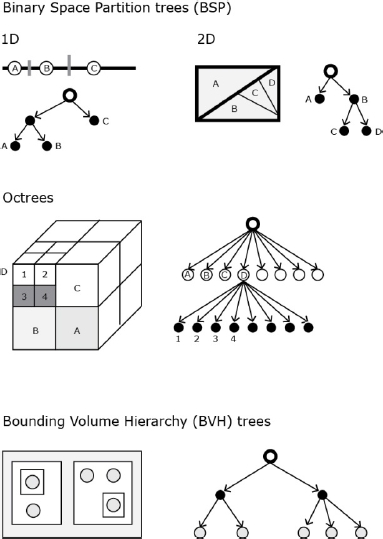
Applied to visual information, there are three important variations of trees:
- – Binary space partition (BSP) tree: while a 2D spatial tree will divide the space by means of 2D splitting lines, a BSP will partition the inner space of volumes into subspaces. Depending on the algorithmic operations, subspaces can be 2D polygons, 3D polyhedra or higher-dimensional polytopes [HUG 14, p. 1084].
- – Octrees: octrees extend the idea of quadtrees from two dimensions to three dimensions. The tree structure consists of nodes pointing to eight children that describe the volume space. The principle is to start from the cube volume that surrounds a model and to recursively subdivide it into smaller cubes. As in the case of quadtrees, each division is performed at the center of its parent.
- – Bounding volume hierarchy (BVH) tree: this structure separates space in nesting volumes by means of axis-aligned boxes (bounding tight clusters of primitives). Its implementation requires first a BSP tree and then boxes form bottom-top (from the leaves to the root). Even though boxes at the same level often overlap in this passage, it has demonstrated better efficiency over octrees and has gained recent popularity for ray tracing and collision detection operations.
To close this section, we should point to the fact that image synthesis considers the generated or modeled graphical object together with the virtual world, or environment, where it exists. For example, in 3D graphics, the data structure scene graph arranges the whole universe of the image, from the scene to the object to its parts.
2.2.4. Algorithms
If we imagine data structures as objects, algorithms then would be the actions allowed on those objects. The close relationship between both can be seized from what we expect to do with our data. Just as in dialectic situations, a data structure is conceived to support certain operations, but algorithms are also designed based on the possibilities and limits of data structures.
Computer scientist Donald E. Knuth defined algorithms simply as a “finite set of rules that gives a sequence of operations for solving a specific type of problem” [KNU 68, p. 4]. In this approach, the notion can be related to others like recipe, process, method, technique, procedure or routine. However, he explains, an algorithm should meet five features [KNU 68, pp. 4–6]:
- – Finiteness: an algorithm terminates after a finite number of steps. A counter example of an algorithm that lacks finiteness is better called a computational method or procedure, for example, a system that constantly communicates with its environment.
- – Definiteness: each step must be precisely, rigorously and unambiguously defined. A counter example would be a kitchen recipe: the measures of ingredients are often described culturally: a dash of salt, a small saucepan, etc.
- – Input: an algorithm has zero or more inputs that can be declared initially or that can be added dynamically during the process.
- – Output: it has one or more quantities that have a relation with the inputs.
- – Effectiveness: the operations must be basically enough so that they could be tested or simulated using pencil and paper. Effectiveness can be evaluated in terms of the number of times each step is executed.
Algorithms have proliferated in computer science and make evident its relationship to mathematics. Because data types are handled as discrete numerical values, an algorithm takes advantage of calculations based on mathematical concepts: powers, logarithms, sums, products, sets, permutations, factorials, Fibonacci numbers, asymptotic representations. Besides those, in visual computing, we also found: algebra, trigonometry, Cartesian coordinates, vectors, matrix transformations, interpolations, curves and patches, analytic geometry, discrete geometry, geometric algebra. The way in which an algorithm implements such operations varies enormously, in the same sense that various people might solve the same problem very differently. Thus, there are algorithms that are used more often than others, not only because they can be used in several distinct data structures, but also because they solve a problem in the most efficient yet simple fashion.
To describe an algorithm, its steps can be listed and written in a natural language, but it can also be represented as mathematical formulae, as flow charts, or as diagrams depicting states and sequences3 (Figure 2.4). The passage from these forms to its actual execution goes through its enunciation as a programming code (the topic of section 2.3.1).

Figure 2.4. Euclid’s algorithm and flowchart representation [KNU 68, pp. 2–3]
Before diving into algorithms for visual information, we briefly review the two broadest types of algorithms used in data in general: sorting and searching.
2.2.4.1. Sorting
Sorting, in the words of Niklaus Wirth, “is generally understood to be the process of rearranging a given set of objects in a specific order. The purpose of sorting is to facilitate the later search for members of the sorted set” [WIR 04, p. 50]. D. E. Knuth exemplifies the use of sorting algorithms on items and collections by means of keys. Each key represents the record and establishes a sort relationship, either a < b, or b < a, or a = b. By the same token, if a < b and b < c, then a < c [KNU 73, p. 5]. There exist many different sorting algorithms and methods; among the most used, we have:
- – Sorting by insertion: items are evaluated one by one. Each item is positioned in its right place after each iteration process of the steps.
- – Sorting by exchange: pairs of items are permutated to their right locations.
- – Sorting by selection: items are separated, or floated, starting with the smallest and going up to the largest.
The first and the most basic algorithms evolved as the amounts and type of data to be sorted increased and differed. Examples of advanced algorithms invented around the 1960s but still in use today are: Donald Shell’s diminishing increment, polyphase merge, tree insertion, oscillating sort; Tony Hoare’s quicksort; J. W. J. William’s heapsort.
2.2.4.2. Searching
Searching is related to processes of finding and recovering information stored in the computer’s memory. In the same form of sorting, data keys are also used in searching. D. E. Knuth puts the problem as: “algorithms for searching are presented with a so-called argument, K, and the problem is to find which record has K as its key” [KNU 73, p. 389]. Generally speaking, there have been two main kinds of searching methods: sequential and binary.
- – Sequential searching starts at the beginning of the set or table of records and potentially visits all of them until finding the key.
- – Binary searching relies in sorted data that could be stored in tree structures. There are different binary searching methods. Knuth already identifies binary tree searching (BTS), balanced trees, multiway trees, and we observe more recent derivations such as red-black trees or left-leaning red-black trees (LLRB) (which were evoked at the end of the last section as an example of esoteric data structure). Anyhow, the overall principle of these searching methods is to crawl the tree in a symmetric order, “traversing the left subtree of each node just before that node, then traversing the right subtree” [KNU 73, p. 422].
We will now discuss some algorithms introduced specifically within the context of visual data. For practical reasons, we continue distinguishing techniques from different fields in visual computing4, and we also relate how these techniques apply on specific data structures.
2.2.4.3. Geometric Transformations
Geometric transformations imply modification of the coordinates of pixels in a given image. They are based consistently on arrays and matrices data structures. They define operations for translating (i.e. moving linearly along the axes), rotating (along two or three axes) and scaling (i.e. dimensioning an image). These techniques can be applied globally – that is, to the entire bitmap image – or only onto smaller layered images contained in the space, such as sprites in 2D graphics or meshes in 3D graphics.
Common variations of these methods include: stretching or contracting, shearing or skewing, reflecting, projecting (rotating and scaling to simulate perspective). More complex methods exist such as nonlinear distortions. In this case, the points are mapped onto quadratic curves resulting in affine, projective, bilinear, twirl, ripple and spherical transformations, for example.
2.2.4.4. Image transformation (image filtering)
The second important family of transformations that are also based on arrays and matrices of pixels are filters. The general idea of filtering is to define a region of pixels inside the image (also called a neighborhood or spatial mask, kernel, template, window), then to perform an operation on that region before applying it to the entire image space [GON 08, p. 167]. There are two main types of filtering in visual computing literature. First, those performed on the image space:
- – Intensity transformations: such as negative transformations, contrast manipulation, and histogram processing.
- – Smoothing filters: used for blurring and noise reduction, either by averaging or ranking (ordering) the pixels in the mask.
- – Sharpening filters: enhance edges by spatial differentiation [GON 08, p. 179].
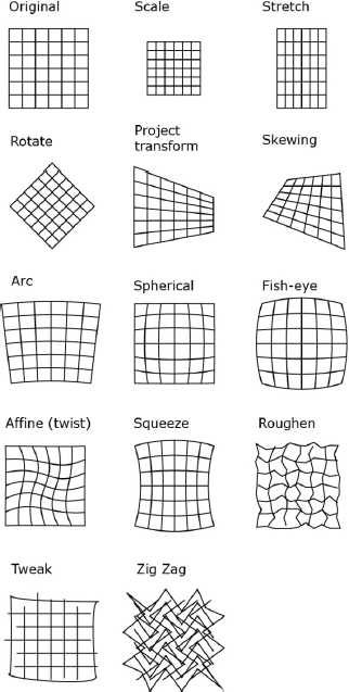
Figure 2.5. Geometrical transformations (created with Adobe Illustrator filters)
Second, there are filters that perform better when the image is viewed as a signal. As with sound frequency and amplitude, images also show variations of visual information that can be associated with frequencies. The standard mechanism to transform image coordinates into frequencies is the Fourier transform.
- – Fourier transform: this helps to determine the amount of different frequencies in a signal. To do this, the surface of the image is first converted to sine and cosine curves. “The values of the pixels in the frequency domain image are two component vectors” [PAR 11, p. 254]. Variations of this transform are discrete Fourier transform or DFT (applied to sampled signals) and the fast Fourier transform or FFT (an optimization of the latter).
- – High-pass filters: these are based on small frequencies; they apply transformations to edges and small regions.
- – Low-pass filter: refer to slow variation in visual information such as big objects and backgrounds.

Figure 2.6. Image filtering. FFT images were produced with ImageJ, all other with Adobe Photoshop
As it might be guessed, some filter operations can be achieved faster in the frequency space than in the image space, and vice versa: particular methods like correlation and convolution5 address those issues. Nowadays, there are new techniques and ongoing research that extend the use of image filtering into specialized fields within the domains of image processing and computer vision dedicated to image enhancement, image correction, image restoration, image reconstruction, image segmentation, image measurement, image and object detection, and image and object recognition. Among many other standalone or combined filters introduced for special uses, we may cite: noise, noise reduction, thresholding, and motion blur.
2.2.4.5. Color quantization (color segmentation)
Color quantization refers to those procedures by which the amount of colors available in a bitmap image is reduced or mapped or indexed to a different scale. Today, this is mainly used for image acquisition (for example, when an image is captured through the camera lens, the colors of the natural world have to be sampled for digital representation) and for image content-based search [PAR 11, p. 399].
Two main categories of methods for color quantization can be identified: 1) the scalar method, which converts the pixels from one scale to another in a linear manner; and 2) the vector method, which considers a pixel as a vector. The latter technique is used more for image quality and counts more efficient algorithms, including: the popularity algorithm (takes the most frequent colors in the image space to replace those which are less frequent); the octree algorithm, which as we saw in the last section is a hierarchical data structure. It partitions the RGB cube consecutively by eight nodes, where each node represents a sub-range of the color space); and the median cut algorithm (similar to the partitions in the octree, but it starts with a color histogram and the representative color pixel corresponds to the median vector of the colors analyzed) [BUR 09, p. 89].

Figure 2.7. Color segmentation. Images were produced with Color Inspector 3D for ImageJ. For a color version of the figure, see www.iste.co.uk/reyes/image.zip
As with the frequency space view, vector-based color segmentations work better with the 3D view of the RGB color space in order to facilitate the evaluation of color distributions and proximities.
2.2.4.6. Image compression
Another family of algorithms that builds on pixel values is dedicated to image storing and transmission purposes. Broadly speaking, the goal of image compression algorithms is to reduce the amount of data necessary to restitute an image. Such algorithms can be classified as lossless or lossy: the former is used to preserve in its entirety the visual information that describes an image, while the latter reduces the file size mainly through three methods [GON 08, p. 547]: by eliminating coding redundancy, by eliminating spatial redundancy, and by eliminating information invisible for human visual perception.
Lossy algorithms have been successfully implemented in image file formats like JPEG and PNG (section 2.3.3 deals with image formats in more detail). The way in which pixel values are handled implies transforming them into code symbols that will be interpreted at the moment of image restitution (the process is called encode/decode; codecs are the programs in charge of performing these operations). PNG files, for example, are based thoroughly on spatial redundancies. The format uses the LZW algorithm (developed by Lempel, Ziv and Welch in 1984) for assigning predefined code symbols to visual information.
On the other hand, formats like JPEG use the Huffman coding algorithm (introduced in 1952 and also used for text compression) in order to determine “the smallest possible number of code symbols” [GON 08, p. 564] based on ordering probabilities. Moreover, just like the Fourier transform, JPEG formats also use a frequency field representation called discrete cosine transform. The difference image describes visual variations “only with cosine functions of various wave numbers” [BUR 09, p. 183] which are ordered by their importance to represent those visual variations (spatial regions, chromatic values, etc.)
2.2.4.7. Image analysis and features
Image analysis also constructs on pixel values. It extends image-processing techniques by taking a different direction towards feature detection and object recognition techniques. The algorithms designed for such tasks analyze a digital space according to two categories: image features and shape features.
- – Image features are those properties that can be measured in an image such as points, lines, surfaces and volumes. Points delimit specific locations in the image (the surrounding area is called keypoint features or interest points, for example, mountain peaks or building corners [SZI 10, p. 207]), while lines are used to describe broader regions based on object edges and boundaries. Formal descriptors for these features are SIFT (scale invariant feature transform) and SURF (speeded up robust features).
- – Shape features constitute the metrics or numerical properties of descriptors that characterize regions inside an image. There are several types, classifications and terminologies of shape descriptors:
- – Geometrical features: they are algorithms to determine the perimeter, area and derivations based on shape size (eccentricity, elongatedness, compactness, aspect ratio, rectangularity, circularity, solidity, convexity [RUS 11, p. 599]).
- – Fractal analysis: mostly used to summarize the roughness of edges into one value. A simple calculation implies starting at any point on the boundary and follow the perimeter around; “the number of steps multiplied by the stride length produces a perimeter measurement” [RUS 11, p. 605].
- – Spectral analysis (Fourier descriptors or shape unrolling): this describes shapes mathematically. It starts by plotting the X and Y coordinates of the region boundary and then converting the resulting values into the frequency field.
- – Topological analysis: these descriptors quantify shape in a structural manner, which means they describe, for example, how many regions or holes between borders are in an image. Algorithms for optical character recognition (OCR) are an example where topological analysis is applied: they describe the topology of characters as a skeleton.
Later in this book, we will show some applications using shape descriptors and we will note that they can be combined. They can also be generalized to 3D shapes and, more recently, they are available as programmatic categories in order to implement machine learning algorithms.
2.2.4.8. Image generation (computational geometry)
These types of algorithm make reference to methods and techniques that generate or synthesize geometric shapes. From a mathematical perspective, a distinction is made between a geometrical and topological description of shapes. Geometry simply defines positions and vertices coordinates, while topology sees the internal properties and relationships between vertices, edges and faces. When pure geometrical description is needed, a set of vertices or an array of positions is enough, but it is common to use a vertex list data structure that organizes the relations between vertices and faces and the polygon. We will now explore prominent techniques for image generation.
- – Voronoi diagrams and Delaunay triangulation: these geometric structures are closely interrelated although they can be studied and implemented separately. Voronoi diagrams are commonly attributed to the systematic study of G. L. Drichlet in 1850 and later adapted by G. M. Voronoi in 1907 [DEB 08, p. 148]. Basically, they divide planar spaces into regions according to a “mark” or “seed” (which can be a given value, or a cluster or values, or a given shape inside an image); the following step consists of tracing the boundaries of regions by calculating equal distances from those “marks”. On its own, the resulting geometry of the diagram can help identify emptier and larger spaces, and also to calculate distances from regions and points (through the nearest neighbor algorithm, for example).
Voronoi diagrams can be extended into Delaunay triangulations by relaying the marker points and tracing perpendicular edges to the boundaries. While there are several triangulation methods, the popularity of Delaunay’s algorithm (named after its inventor, mathematician Boris Delone) resides in its efficiency for reducing triangles with small angles (a situation that is desired for their subsequent uses such as creating polygonal and polyhedral surfaces)6.
- – Particle systems: these are typically collections of points where each dot is independent from the others, but follows the same behavior. More clearly, single points have physics simulation attributes such as forces of attraction, repulsion, gravity, friction and constraints such as collisions and flocking clusters. It is documented that the term “particle system” was coined in 1983 by William Reeves after the production of visual effects for the film Star Trek II: the wrath of Khan at Lucasfilm [SHI 12, ch. 4]. As in that case, particle systems are used to generate and simulate complex objects such as fire, fireworks, rain, snow, smog, fog, grass, planets, galaxies or any other object composed of thousands of particles. Because particle systems are often used in computer animation, algorithms for velocity and acceleration are also used. Common methods involve considering particles as vectors and adapting array list data structures to keep track and ensure collision detection procedures.
- – Fractals: these are geometric shapes that, following the definition by mathematician Benoît Mandelbrot who coined the term in 1975, can be divided into smaller parts, but each part will always represent a copy of the whole. In terms of image generation, fractals use iteration and recursion. That means a set of rules is applied over an initial shape and, as soon as it finishes, it starts again on the resulting image. Famous examples of fractal algorithms are the Mandelbrot set, the Hilbert curve, the Koch curve and snowflake.
Fractals have been adapted into design programs by using grammars. The idea of grammar-based systems comes from botanist Aristid Lindenmayer, who in 1968 was interested in modeling the growth pattern of plants. His L-system included three components: an alphabet, an axiom, and rules. The alphabet is composed of characters (e.g. A, B, C), the axiom determines the initial state of the system, and the rules are instructions applied recursively to the axiom and the new generated sentences (e.g. (A→AB)) [SHI 12, ch. 8].
- – Cellular automata: these are complex systems based on cells that exist inside a grid and behave according to different states of a neighborhood of cells. The states are evaluated and the system evolves in time. The particularity of these systems is their behavior: it is supposed to be autonomous, free, self-reproducing, adapting, and hierarchical [TER 09, p. 168]. Uses and applications of cellular automata can be seen in video games (such as the famous Game of Life by John Conway in 1970), modeling of real-life situations, urban design, and computer simulation.
- – Mesh generation: procedures of this kind are related to 3D reconstruction techniques, tightly bounded to surface and volumetric representation as well as mesh simplification methods. Mesh generation is commonly associated with creating 3D models, useful in medical imaging, architecture, industrial design, and recent approaches to 3D printing. The design of these algorithms first considers the kind of input data because clean mesh surfaces are not always the starting points (i.e. planar, triangle-based, with explicit topology that facilitate interpolation or simplification).
- – Points: these algorithms consider scattered points around the scene. They can be seen as generating a particle system as a surface. A simple method tends “to have triangle vertices behave as oriented points, or particles, or surface elements (surfels)” [RUS 11, p. 595].
- – Shape from X: this is a generalization of producing shapes from different sources, for example, shades, textures, focuses, silhouettes, edges, etc. The following section will give an overview of shading and texturing, but the principle in here is to reconstruct shapes by implying the illumination model and extracting patterns of texture elements (called textels).
- – Image sequences: let’s suppose we have a series of images positioned one after another along the Z-axis, like a depth stack. Algorithms have been designed to register and align the iterated closest matches between the surfaces (the ICP algorithm). Then, another algorithm such as the marching cubes can help generate the intersection points between the surface and the edges of cubes through vertices values. In the end, a triangulation method can generate the mesh tessellation. Of course the differences between a clean mesh surface and one generated as an isosurface reside in the complexity and quantity of vertices and edges. It is precisely for these cases that mesh decimation or mesh triangulation are used to reduce and simplify the size of models.
2.2.4.9. Image rendering
Once an object has been generated, either within a 2D or a 3D world, there is a necessary passage from the geometrical information to the visual projection on the screen. In other words, we go from image pixel values to “screen pixel values”, a process generally called image rendering. There are actually two main rendering methods, rasterization and ray casting. Both take into account more visual information than geometry.
- – Viewing and clipping: image viewing is related to the virtual camera properties. This is the same as choosing the right angle, position, tilt and type of lens before we take a photograph. In the case of visual information, image viewing consists of four main transformations: position, orientation, projection (lens, near and far plans, or view frustrum), and viewport (shape of the screen). In parallel, image clipping relates to eliminating geometrical information outside the viewing volume of the scene. Algorithms such as Sutherland and Hodgman are adapted to clip polygons [HUG 14, p. 1045].
- – Visible surface determination: this family of algorithms is also called hidden surface removal depending on the literature and specificities ([HEA 04] argues that the case of wire-frame visibility algorithms might invigorate the term visible surface determination as it is more encompassing). Anyhow, their main goal is to determine which parts of the geometrical information will be indeed shown on the screen. Although there are abundant algorithms depending on the hardware, software or type of geometry, we can exemplify two broad approaches. On the one hand, the family of image space methods, such as the depth-buffer or z-buffer algorithms, builds on hardware graphics power to trace, screen pixel by screen pixel, all polygons existing in the virtual world, and showing only those closest to the view point. On the other hand, the family of object space methods, such as the depth sorting or the painter’s algorithm, first sort objects according to the view point. Then, they render from the farthest object to the closest, like layers on a canvas or celluloid sheets. It is interesting to note that the latter method is currently implemented in graphical user interfaces (see section 2.3.2).
- – Lighting and shading: objects and meshes do not have only solid colors to be visible. Mainly for photorealistic objectives, the visual aspect of surfaces can be considered a combination of colors, textures and light that bounces around the scene. This is essentially what we call shading. The model of light underlying shading algorithms consists of the light source itself (its location, intensity, and color spectrum) as well as its simulated behavior on surfaces:
- - Diffuse reflection (Lambertian or matte reflection): distributes light uniformly in all directions.
- - Specular reflection (shine, gloss or highlight): mostly depends on the direction of the bouncing light.
- - Phong shading: a model that combines diffuse and specular with ambient illumination. It follows the idea that “objects are generally illuminated not only by point light sources but also by a general diffuse illumination corresponding to inter-reflection” [SZI 10, p. 65].
The BDRF (bidirectional reflectance distribution function) is a model that also takes into account diffuse and specular components; nevertheless, more recent programming environments embrace vertex and fragment shaders functions that allow for integrating more complex models in real-time rendering.
- – Texturing: another visual feature of objects is their simulated texture. That means that instead of geometrically modeling the tiniest corrugation, we use 2D images as textures that simulate such depth. Lastly, the 2D image is handled as an array whose elements are called textels. In terms of [ANG 12, p. 366]: “The mapping algorithms can be thought of as either modifying the shading algorithm based on a 2D array (the map), or as modifying the shading by using the map to alter surface parameters, such as material properties and normal.” There are three main techniques:
- – Texture mapping: this is the texture in its common sense meaning. One way to do this is to associate a texture image with each triangle of the mesh. Other methods unwrap the surface onto one or more maps (called UV mapping).
- – Bump mapping: the goal of this technique is to alter the normal vectors of models in order to simulate shape imperfections (recall that normal vectors designate the direction of faces according to the convex hull).
- – Environment mapping: this refers to techniques where an image is used to recreate how objects in the scene reflect light, but without tracing the actual rays of light. Most of the time, these maps are built on polar coordinates or parametric coordinates [HUG 14, p. 549].
- – Ray tracing: in contrast to the last paragraph, these algorithms actually trace the path of light rays in a scene. The method consists of starting from a screen pixel and then searching for intersections with objects. Of course although in the physical world there are endless light bounces, in here it is necessary to delimit the depth of level of intersections (often three levels). In the end, it is possible to “combine the color of all the rays which strike our image plane to arrive at the final color for each pixel” [GOV 04, p. 179]. An alternative contemporary method to ray tracing is called radiosity, which is inspired by thermal heat transfer to describe light as energy emitters and receivers.
2.3. Visual information as texts
The next level in our generative trajectory refers to texts, which we understand in a broader sense. Texts have to do with configurations that are made out of the entities encountered at the fundamental level (data types, data structures, and algorithms). Texts are enunciations: manifest interpretations of how and which information is present (to the emitter and the receiver). Thus, for text to be comprehensible and transferable, it should follow some syntactic and semantic rules shared by the sender and the receiver. Moreover, as occurs with texts in general (for example, a narrative prose and a poem are structurally different from scientific texts), programming codes have writing styles that reflect on computation models underlying the representation they make of data.
In this section, we describe how the units of the fundamental level are manifested in the form of text. We have chosen three main entry points. The first is in terms of programming code, and we will discuss programming languages and their categorizations. The second concerns graphical user interfaces. At the end of the section, we take a look at file formats as they can also be seen as texts.
2.3.1. Programming languages
In section 2.2.1, we evoked different levels of programming languages. At the closest part to the binary code (the lowest level), there are machine languages. Then, on top of them, we identify assembly languages, which facilitate programming by conventionalizing instructions, that is, using mnemonic conventions instead of writing binary code. A third layer consists of high-level programming languages, which assist in focusing on the problem to be tackled rather than on the lower-level computing details (such as memory allocation). These languages are essentially machine-independent (we can write and execute them in different OS) and generally can be regarded as compiled or interpreted. Compiled languages are commonly used for developing standalone applications because the code is converted into its machine language equivalent. On the other hand, interpreted languages use a translator program to communicate with a hosting software application (that means the code executes directly on the application). Examples of the first category include languages like Java and C++, while the second is associated with languages such as JavaScript and Python, among many others.
Programming languages provide the means to manipulate data types and data structures as well as to implement algorithms. Computer scientist Niklaus Wirth has observed analogies between methods for structuring data and those for structuring algorithms [WIR 04, p. 129]. For instance, a very basic and recurrent operation in programming is to “assign an expression’s value to a variable”. This is done simply on scalar and unstructured types. Another pattern is “repetition over several instructions”, written with loop sentences on an array structure. Similarly, the pattern “choosing between options” would build on conditional sentences using records. As we will see, in programming terms, sentences are called statements (also known as commands or instructions): they contain expressions (the equivalent of text phrases), and they can be combined to form program blocks (the equivalent of text paragraphs).
In this section, we will observe the overall characteristics of programming languages, from the syntactic, semantic and pragmatic point of view. Then we will present some programming styles (also called paradigms or models) and conclude by revisiting major programming languages for visual information.
2.3.1.1. Syntactics, semantics and pragmatics
In contrast to natural languages such as English, French, Spanish, etc., programming languages are formal languages. That means they are created artificially to describe symbolic relationships, like in mathematics, logics, and music notation. One way of studying programming languages has been to distinguish between the syntactic, semantic and pragmatic dimensions, just as they were originally envisioned by semiotician Charles Morris (see section 2.1) and early adopted in computer science literature [ZEM 66].
Syntactics refers broadly to the form of languages. We can say it encompasses two main parts: the symbols to be used in a language, and their correct grammatical combinations.
The first part of syntactics is known as concrete syntax (or context-free grammars); it includes the character set (alphanumerical, visual or other alphabet), the reserved special words (or tokens, which are predefined words by the language), the operators (specific symbols used to perform calculations and operations), and grouping rules (such as statement delimiters – lines or semicolons – or delimiter pairs – parentheses, brackets, or curly brackets).
The second part is named syntactic structure or abstract grammar. It defines the logical structure or how the elements are “wired together” [TUR 08, p. 20]. This part gives place to language constructs where we can list, ranging from simple to complex: primitive components, expressions, statements, sequences and programs. Expressions like “assigning value to a variable” demand using the dedicated token for the data type, the identifier of the variable, an assignment operator and the assigned value (for example, int num = 5). Regarding statements, there are several types (conditional, iteration and case), each identified with their own tokens (if-else, for or while, switch) and delimited by grouping rules. A statement is considered by many languages as the basic unit of execution.
Semantics refers to the meaning of programs at the moment of their execution. In other words, it is about describing the behavior of what language constructs do when they are run. Because programs are compiled or interpreted on machine and layers of software, it is said that semantics depends on the context of execution or the computational environment. Although most of the time we express the semantics in natural language prose as informal description (as it occurs in language references, documentation, user’s guides, the classroom, workshops, etc.), there are a several methods to formalize the semantics of programming language, which are mainly used for analysis and design.
Even though it is not our intention to deal with semantic issues, we only evoke two common methods for specifying programming languages. First, denotational semantics, which explains meaning in terms of subparts of language constructs. And, complementary, operational semantics, which observes language constructs as a step-by-step process. Examples of programming language subparts are: 1) the essential core elements (the kernel); 2) the convenient constructs (syntactic sugar); and 3) the methods provided by the language (the standard library) [TUR 08, p. 207]. Examples of operations at execution are naming, states, linking, binding, data conversions, etc. Together, these methods are useful for identifying and demonstrating language properties (for instance, termination7 or determinism8).
Before tackling pragmatics, we illustrate two practical cases of syntactics and semantics at the heart of most programming languages. Table 2.4 summarizes different operators: the symbol and its meaning at execution. Table 2.5 extends operators by showing their implementation, from a mathematical notation into programming language syntax. We have chosen JavaScript language syntax for both the tables.
Table 2.4. Common operator symbols and their description in the JavaScript language
| Operator symbol | Description |
| + | Addition |
| - | Subtraction |
| * | Multiplication |
| / | Division |
| % | Modulus (division remainder) |
| ++ | Increment |
| -- | Decrement |
| == | Equal to |
| === | Equal value and equal type |
| != | Not equal |
| !== | Not equal value or not equal type |
| > | Greater than |
| < | Less than |
| >= | Greater than or equal to |
| <= | Less than or equal to |
| && | And |
| || | Or |
| ! | Not |
Pragmatics refers to the use and implementation of programming languages. It has to do with the different forms of solving a problem, like managing the resources available in the most efficient way (memory, access to peripherals). In computer science literature, pragmatics is associated with programming models (also referred to as programming styles and programming paradigms).
Table 2.5. From mathematical notation to programming syntax, adapted from Math as code by Matt DesLauriers9. A reference of mathematical symbols for UTF-8 formatting is also available online10
| Mathematical notation | Description | Programming code |
| √(x)2 = x i = √-1 |
Square root. Complex numbers. JavaScript requires an external library such as MathJS. |
Math.sqrt(x); var math = require(‘mathjs’); var a = math.complex(3, −1); var b = math.sqrt(−1); math.multiply(a,b); |
| 3k o j | Vector multiplication. Other variations are: Dot or scalar product of a vector (K o j) and cross product k × j. |
var s = 3; var k = [ 1, 2 ]; var j = [ 2, 3 ]; var tmp = multiply(k, j); var result = multiplyScalar(tmp, s); function multiply(a, b) { return [ a[0] * b[0], a[1] * b[1] ] } function multiplyScalar(a, scalar) { return [a[0] * scalar, a[1] * scalar ] } |
| Sigma or summation. Some derivations are: |
var sum = 0; for (var i = 1; i <= 100; i++) { sum += i } |
|
| Capital Pi or big Pi. | var value = 1; for (var i = 1; i <= 6; i++) { value *= i; } |
|
| |x| | Absolute value. | Math.abs(x); |
| ||v|| | Euclidean norm. “Magnitude” or “length” of a vector. |
var v = [ 0, 4, −3 ]; length(v); function length (vec) { var x = vec[0]; var y = vec[1]; var z = vec[2]; return Math.sqrt(x * x + y * y + z * z); } |
| |A| | Determinant of matrix A. | var determinant = require(‘glmat2/determinant’); var matrix = [ 1, 0, 0, 1 ]; var det = determinant(matrix); |
| â | Unit vector. | var a = [ 0, 4, -3 ]; normalize(a); function normalize(vec) { var x = vec[0]; var y = vec[1]; var z = vec[2]; var squaredLength = x * x + y * y + z * z; if (squaredLength > 0) { var length = Math.sqrt(squaredLength); vec[0] = vec[0] / length; vec[1] = vec[1] / length; vec[2] = vec[2] / length; } return vec; } |
| A ={3, 9, 14}, 3 ∈ A | An element of a set. | var A = [ 3, 9, 14 ]; A.indexOf(3) >= 0; |
| Set of real numbers. | function isReal (k) { return typeof k === ‘number’ && isFinite(k); } |
|
| Functions can also have multiple parameters. | function length (x, y) { return Math.sqrt(x * x + y * y); } |
|
| Functions that choose between two “sub-functions” depending on the input value. | function f (x) { if (x >= 1) { return (Math.pow(x, 2) - x) / x; } else { return 0; } } |
|
| The signum or sign function. | function sgn (x) { if (x < 0) return −1; if (x > 0) return 1; return 0; } |
|
| cos θ sin θ |
Cosine and sine functions. | Math.cos(x); Math.sin(x); |
| f′(x) = 2x | A value similar to another, while keeping the same name. It can describe the “next value” after some transformation. | function f (x) { return Math.pow(x, 2); } function fPrime (x) { return 2 * x; } |
| Floor and ceil functions to round float numbers. | Math.floor(x); Math.ceil(x); |
|
| A ⇒ B | Used in logic for material implication. That is, if A is true, then B is also true. | if (A === true) { assert(B === true); } |
| k ≫ j | Significant inequality. That is, k is an order of magnitude larger than j. | orderOfMagnitude(k) > orderOfMagnitude(j); function log10(n) { return Math.log(n) / Math.LN10; } function orderOfMagnitude (n) { return Math.trunc(log10(n)); } |
| k > 2 ∧ k < 4 ⇔ k = 3 | Logical conjunction ∧. Analogous to operator AND. | if (k > 2 && k < 4) { assert(k === 3); } |
| A ∨ B | Logical disjunction ∨. Analogous to operator OR. | A || B |
| x ≠ y ⇔ ¬ (x = y) | Symbols ¬, ~ and ! are used to represent logical NOT. | if (x !== y) { assert(!(x === y)); } |
| x ∈ [0,1]3 | Intervals. Numbers restricted to some range of values, e.g. a point x is in the unit cube in 3D. Also related are set operations: union ∪, intersection ∩ and difference −. |
var nextafter = require(‘nextafter’) var a = [nextafter(0, Infinity), nextafter(1, -Infinity)]; var b = [nextafter(0, Infinity), 1] ; var c = [0, nextafter(1, -Infinity)] ; var d = [0, 1] ; |
From this standpoint, programming languages have been divided into styles by the way in which they adapt a computational model. For example, two prominent paradigms used today are the imperative model and the object-oriented model. The former is implemented by procedural languages and is based on the use of sequences or blocks to compute step-by-step procedural hierarchies. The latter defines objects that have properties and behaviors previously declared as a data class. Classes thus have class variables and class methods, which can also be nested and combined with other classes (something called inheritance). Other paradigms that we might cite are: functional, logic, declarative, concurrent11 and, more recently, multi-paradigms and emerging ones such as reactive programming. Of particular importance for our study will be the visual programming approach, which adds functionalities of graphical user interfaces to languages (see next section 2.3.2).
Let’s now present some of the main programming languages that are used to handle visual information, namely Java, C++, Python, JavaScript and OpenGL. These languages are of course very popular and too vast; they are used for a large number of different applications. The following account has no intention to introduce programming techniques, but only to have a glance at the main characteristics and general behaviors, for “a programmer is greatly influenced by the language in which programs are written” [KNU 68, p. ix]. In the next chapter, we will explore concrete implementations for specific image-interface scenarios.
2.3.1.2. Java
Java 1.0 was introduced in 1996 by Sun Microsystems. At the moment of writing these lines, its current version is Java 8, maintained by Oracle Corporation (which acquired Sun). In little more than 20 years, the Java programming language has grown from roughly 200 classes organized in 8 packages to more than 4000 and 200 packages (we will see later what classes and packages are).
Java can be seized as a programming ecosystem that includes the language specification, a compiler, the run-time environment, and its various APIs (application programming interfaces) that extend its basic functionalities. Moreover, because Java is general-purpose, there are actually several versions: Java Mobile Edition (Java ME), Java Standard Edition (Java SE), Java Enterprise Edition (Java EE) and Open Java Development Kit (JDK). However, vendors and companies (Apple, IBM, Red Hat, among others) have worked together on interoperability standards to maximize compatibility.

Figure 2.8. Network graph of main tokens, statements and types in Java, Python, C++ and JavaScript programming languages. For a color version of the figure, see www.iste.co.uk/reyes/image.zip
As with the other programming languages, the Java syntax can be seen in a hierarchical categorization. From simple to complex, we may list: tokens, data types, statements, methods, classes, packages and programs. In Figure 2.8, we summarize the differences and similarities between tokens, primitive types, and statements supported in the languages reviewed here12. For Java in particular, the syntax levels are based on 53 tokens and 8 primitive types.
One of the strengths of Java is the manner in which it supports object-oriented programming, where methods and classes play a major role. A method has been defined as “a named sequence of Java statements that can be invoked by other Java code. When a method is invoked, it is passed zero or more values known as arguments.” [EVA 15, p. 66], and classes are “a named collection of fields that hold data values and methods that operate on those values” [EVA 15, p. 72].
The idea of classes is built on the concept of data structures. Classes define new types by combining several primitive types within a constructor, which is a block of code that specifies the properties and behaviors of the class. However, a class exists only virtually, as a formal and abstract rule that needs to be materialized. The instance of a class is called an object which holds the same properties and behaviors of its class, and which can be instantiated indefinitely. Another interesting part of objects is that they can be nested and can inherit properties from other classes.
In the following upper level of syntax complexity, classes are grouped into packages. In Java, all predefined packages start with the token “java”, such as java.util, java.lang, and it is also possible to create our own packages. The highest level of syntax is a program: it consists of one or several files of source code. If a Java file contains a class, it is expected to be named according to that class (e.g. Filename.java would contain the class Filename). Then, when they are compiled, the file is transformed into Java byte code, creating a file with extension “.class” (i.e. Filename.class) that can be executed by the run-time environment for a given type of computer processor.
Among the many APIs available to extend the basic functionalities of Java, there are mainly two devoted to synthesizing images: Java 2D13 and Java 3D14. Furthermore, there is also a binding for the OpenGL library called JOGL15 (later in this section, we present OpenGL). Finally, Java is also the foundation for the development of seminal programming environments dedicated to working with visual information, among others: RStudio, ImageJ and Processing.
2.3.1.3. C++
C++ was initiated in 1985 at Bell/AT&T and was standardized in 1988 by ISO/IEC. Although it was initially inspired by the C language with the intention to facilitate some tasks, it has grown separately and can be considered a different language. Currently, the latest published version is C++14 (from 2014), maintained by the Standard C++ Foundation (a non-profit organization with members from Google, Microsoft, Intel, among others).
C++ is a compiled language that might feel of lower level than Java because of its abstractions (e.g. access to memory management, pointers and preprocessing). It supports a generic programming paradigm that constructs mainly on procedural and object-oriented (recall Pragmatics in section 2.3.1.1). To work with C++ programming code, it is necessary to have an editor and a compiler, or an IDE (integrated development environment, offering an editor, a compiler, and a file management system in a bundle such as Eclipse16 or NetBeans17, both multi-language, multiplatform, and freely available tools). Anyhow, there also exist commercial implementations of C++ that extend the primary functions of the language.
C++ comprises 74 tokens and 15 primitive types. As we mentioned before, Figure 2.8 shows a map of relationships of types, tokens and statements used in languages of this section. Besides that, the hierarchical syntax of C++ is similar to Java, from expressions to statements, classes, templates, the standard library, projects and programs.
The particular notion of template is similar to the classes and objects behavior in Java; it makes reference to a model for creating classes or functions as instances of the template. However, in C++ template-based programming, a class or a function can be defined “independently of its parameters (which can be values, types, or even other templates)” [LIS 03, p. 174]. The C++ standard library concerns types, macros, functions and objects that can be used in programs: these all are called headers. In C++14, there are 51 headers and it is mandatory to add the directive #include, for example: #include <header> (third-party libraries are also called projects, like Boost18 and many others19).
At compilation time, the header is entirely replaced by the content of the file to which it makes reference. A C++ program may consist of several files, each containing zero, one or more headers. Conventionally, files comprising headers only bare the file extension .h or .hpp, while their implementation is in files with extension .c or .cpp.
The main form in which C++ handles visual information is through libraries (also called C++ projects). One of the most famous is the OpenGL library for computer graphics, but there are others specially designed for computer vision (OpenCV), image processing (Magick++), and artistic images (Cinder and OpenFrameworks). Given its lower level nature, ultimately many software applications can be developed or extended with C++, including Pure Data, RStudio and MATLAB.
2.3.1.4. Python
Python was initiated by Guido van Rossum in 1990, and it is currently maintained by the non-profit Python Software Foundation. It supports procedural and object-oriented programming styles and is considered of higher level than C++ and Java mainly because it is run on an interpreter and does not require any further compilation (thus it is known as an interpreted language).
Python can also be seen as a software ecosystem containing the language, an interpreter, and a series of extension modules. There are two main modes of using Python: Classic Python (CPython), which is the most widely used, and Jython, which is an implementation of the language for Java. In the first case and for basic operations, it is recommended to install the Python IDE (called IDLE) that offers an editor, an interpreter and a debugger available for multiple platforms. For complex operations using different libraries and packages, [MON 16] recommends to install a Python distribution like Anaconda20.
The syntax of Python programs follows the previously explored principles, constructing from expressions to statements, modules, packages and programs. The 33 keywords reserved in Python 3 are summarized in Figure 2.8. In Python terminology, sets and dictionaries would be the equivalents to lists and arrays in other languages. Actually, dictionaries support mapping; therefore, they can be thought of as associative arrays (the equivalent of “map,” “hash table,” or “hash” in other languages). Another difference that should be mentioned is that lines of code written in Python are equal to physical lines. That means there is no semicolon to indicate the end of a statement, but it is rather the end of the line itself. The same situation occurs with indentation, which is used to “express the block structure of a program” [MAR 06, p. 34].
One of the central notions in Python is the module. Modules are chunks of programming code, stored in different files with the idea of making them reusable and portable. Modules can be called between them using the import statement (creating a namespace to access the properties of such modules) and, because in Python all types are objects, “a function can return a module as the result of a call. A module, just like any other object, can be bound to a variable, an item in a container, or an attribute of an object” [MAR 06, p. 140]. The standard library has predefined objects known as built-ins (hence, they do not require the import statement, contrary to extensions), covering 68 functions dedicated to types and algorithms.
A complete Python program may have different files. The file extension used for modules is .py (.pyc is also used for compiled files in bytecode). Given the popularity of the language, a large number of libraries exist as extension modules that can be bundled in packages. Of special interest to this book is PIL (Python Imaging Library) and its derivative Pillow adaptation. Furthermore, it is often the case to use a visual information library together with other packages: Tkinter for graphical user interfaces, SciPy for mathematics and graphics, Panda3D for games, to mention some.
2.3.1.5. JavaScript
JavaScript was designed by Brendan Eich at Netscape. Strictly speaking, the name JavaScript is protected by Sun Microsystems (acquired by Oracle in 2010), but the standard version received the name ECMAScript in 1997 (after the European Computer Manufacturer’s Association). Currently, JavaScript 1.5 is of the same ECMAScript 5 standard, though the most recent version is 7, released in 2016.
JavaScript is largely known to be the scripting language of the Web, as it is an interpreted, high-level language that can be run on web browsers (although there are derivations of the language used to script software applications such as ExtendScript for Adobe Photoshop, Illustrator, and After Effects). JavaScript has evolved to support several programming styles (functional and object-oriented) thanks to its API for understanding and manipulating a document model (most notably HTML).
The overall lexical structure of JavaScript is inspired from Java. It delimits 29 keywords to formulate expressions and statements. Besides the five primitive types (numbers, strings, Boolean, and null or undefined), everything else can be an object. For example, basic arithmetic expressions combine values with operators (+, −, /, *), but when it is necessary to perform more complex operations, we have to use the Math object and its predefined methods: Math.sin(), Math.cos(), Math.floor(), Math.random(), etc.
There are three important kinds of objects in JavaScript: arrays, functions and objects. Arrays represent an ordered collection of elements with dedicated methods to access them. It is interesting to note that elements of an array can be of different types, making it possible to create complex data structures such as arrays of arrays, arrays of objects, multidimensional arrays, etc. Functions are objects with “executable code associated with it” [FLA 11, p. 30]. They can be launched asynchronously from other objects and return a computed value, that could be yet another function. Finally, functions are widely used to create new objects via constructors, in the fashion of object-oriented programming. For practical matters, there are several predefined classes of objects such as Date, RegExp and Error, which help create methods and objects that represent dates, regular expressions and syntax bugs at runtime, respectively.
As can be guessed, objects in JavaScript constitute the main component of the language. We have already said that objects can have properties and methods of different types and that can also be inherited and nested. When JavaScript is run on web browsers, for example, it starts by creating a model of the document (the DOM, or Document Object Model). But the document is already included in a larger object, which is the browser window. The Window object allows access to properties such as name, innerWidth, innerHieght, screenLeft, screenTop, etc., and methods such as alert(), scrollTo(), prompt(), confirm(), etc.21 Then, at the Document level, the object describes the HTML elements displayed as the content of the page through methods like getElementById()22. Further down the Document object, there is the Element object, which distinguishes HTML elements individually. This functionality is important for manipulating visual attributes associated with styles defined in the Cascade StyleSheets (CSS) standard but also to event handler properties triggered by input devices (e.g. typing a key of the keyboard, click or double-clicking the mouse). Besides Document and Element objects and the Window object, there are also properties and methods for Location23, Screen24, Navigator25 and History26 objects.
A complete JavaScript program might consist of one or more files recognized with the file extension js. Within a web browser context, .js files can be added to an HTML document via the script tag or invoked with the javascript: protocol as an attribute of an HTML element (for instance, <button onclick=“javascript:hello();”>). More recently, JavaScript programs have gained popularity as distributed in the form of “bookmarklets”. These are .js files stored in a server and added as a bookmark to a browser. Then, the browser executes the code “as if it were a script on the page and can query and set document content, presentation, and behavior” [FLA 11, p. 316]. Finally, it is also possible to place the JavaScript code within an HTML document itself, without any reference to external files.
Regarding visual information, JavaScript on the web takes advantage of two main technologies: on the one hand, the HTML5 <canvas> element and, on the other, the SVG (Scalable Vector Graphics) language. HTML5 canvas introduced a drawing API (developed by Apple for Safari 1.3 in 2006) that defines methods for graphics such as lines, curves, polygons, text, shadows, gradients, images and pixel manipulation (these shapes also include 15 visual properties such as lineWidth, fill, shadowColor, etc.). From this perspective, graphics can be considered similar to pixel-based images or bitmaps because they exist within the 2D context of the canvas tag (specifying the width and height of the visible space). Conversely, SVG is a vector image format based on XML, that is, images are structured like a tree, similar to the HTML DOM. Of course, the SVG model varies from that in HTML, but it is worth noting that basic shape elements such as <circle>, <rect>, <line>, or <polygon> can also be grouped and nested into <path> or <g> tags, thus creating the tree-like structure. SVG files have the file extension .svg, natively supported by browsers and software applications like Adobe Illustrator or Photoshop (as smart object). Table 2.6 compares the visual properties that can be accessed with Canvas and SVG, and OpenGL.
The graphics possibilities of the web do not rely exclusively on <canvas> and SVG. As browsers evolve, CSS3 becomes tightly integrated, supporting animation and 3D graphics. Furthermore, HTML5 defines native support for <audio> and <video>, opening access to multimedia file formats to communicate with the HTML DOM (for example, via media events like playing, ended, or volumechange among a total of 22 events and recent recommendations such as WebRTC).
One final word regarding web graphics is the recent support of the OpenGL library. OpenGL ES (Embedded Systems) was adapted from the OpenGL specification in order to operate in consoles, phones, devices, vehicles and web browsers. WebGL is the name given by the Khronos Group to the 3D graphics API. While the first version of WebGL was released in 2011, based on OpenGL ES 2.0 (published in 2008), the second version appeared in 2017 and adopts OpenGL ES 3.0 (published in 2015). JavaScript can use the WebGL API via the <canvas> element. Because OpenGL ES 2.0 specifies shader-based graphics, WebGL also implements vertex and fragment shaders. This is generally a difficult task since the language gets closer to the level of Graphical Processing Units (GPU); thus, several JavaScript libraries have emerged (such as three.js27 or PhiloGL28).
Table 2.6. List of visual attributes in CSS, SVG and OpenGL
| Canvas29 | SVG30 | OpenGL31 |
| addColorStop(), arc(), arcTo(),beginPath(), bezierCurveTo(), clearRect(), clip(), closePath(), createImageData(), createLinearGradient(), createPattern(), createRadialGradient(), data, drawImage(), fill(), fillRect(), fillStyle, fillText(), font, getImageData(), globalAlpha, globalCompositeOperatio n, height, isPointInPath(), lineCap, lineJoin, lineTo(), lineWidth, measureText(), miterLimit, moveTo(), putImageData(), quadraticCurveTo(), rect(), rotate(), scale(), setTransform(), shadowBlur, shadowColor, shadowOffsetX, shadowOffsetY, stroke(), strokeRect(), strokeStyle, strokeText(), textAlign, textBaseline, transform(), translate(), width | alignment-baseline, attributeName, attributeType, azimuth, baseFrequency, baseline-shift, baseProfile, begin, bias, calcMode, class, clip, clip-path, clip-rule, color, color-interpolation, color-interpolation-filters, color-profile, color-rendering, contentScriptType, contentStyleType, cursor, cx, cy, diffuseConstant, direction, display, dominant-baseline, dur, dx, dy, edgeMode, elevation, end, fill, fill-opacity, fill-rule, filter, filterRes, flood-color, flood-opacity, font-family, font-size, font-size-adjust, font-stretch, font-style, font-variant, font-weight, from, fr, fx, fy, gradientTransform, height, href, k1, kernelMatrix, kernelUnitLength, kerning, keySplines, keyTimes, lengthAdjust, letter-spacing, lighting-color, limitingConeAngle, local, marker-end, marker-mid, marker-start, markerHeight, markerUnits, markerWidth, mask, maskContentUnits, maskUnits, max, min, opacity, operator, order, overflow, overline-position, overline-thickness, paint-order, pathLength, patternTransform, pointer-events, points, pointsAtX, pointsAtY, pointsAtZ, preserveAlpha, preserveAspectRatio, r, radius, refX, repeatCount, repeatDur, restart, result, rx, ry, scale, seed, shape-rendering, specularConstant, specularExponent, stdDeviation, stitchTiles, stop-color, stop-opacity, strikethrough-position, strikethrough-thickness, stroke, stroke-dasharray, stroke-dashoffset, stroke-linecap, stroke-linejoin, stroke-miterlimit, stroke-opacity, stroke-width, style, surfaceScale, tabindex, targetX, targetY, text-anchor, text-decoration, text-rendering, textLength, to, transform, type, underline-position, underline-thickness, values, version, viewBox, visibility, width, word-spacing, writing-mode, x, x1, x2, xlink:href, xlink:show, xlink:title, y, y1, y2 | glutInitDisplayMode glColor glIndex glutSetColor(); glEnable(); glBlendFunc (); glEnableClientState(); glColorPointer(); glIndexPointer(); glPointSize(); glLineWidth(); glEnable(); glEnable(); glLineStipple(); glPolygonStipple(); glPolygonMode glEdgeFlag glFrontFace glEnable glGet glPushAttrib glPopAttrib(); |
2.3.1.6. OpenGL
The first version of OpenGL was introduced in 1994 by Silicon Graphics. It was a major achievement in separating software from hardware regarding graphics packages (or Graphics Libraries, GL), in the same line as DirectX and VRML (Virtual Reality Modeling Language). Today, OpenGL is maintained by the non-profit Khronos Group (current release is 4.5) and is widespread across multiple platforms and devices (through, as we sought, OpenGL ES and WebGL).
Technically speaking, OpenGL is not a programming language, but rather a library designed to support 3D and 2D graphics programs. As a matter of fact, it is intended to be independent of any language, yet offers bindings for at least the most common programming languages that we have seen before (Java, C++, Python, JavaScript). Thus, the programmatic capabilities of graphics will depend on the hosting system and language in which OpenGL is implemented.
The syntax of OpenGL describes more than 500 commands. The function names pertaining to the core library can be recognized by the prefix gl. In an analogous manner, the built-in data types contain the prefix GL: GLbyte, GLshort, GLint, GLfloat, GLdouble, GLboolean. Being a multi-purpose library, there are no descriptions of models and surfaces; therefore, it is necessary to construct them programmatically from basic geometry: GL_POINTS, GL_LINES, GL_LINE_STRIP, GL_LINE_LOOP, GL_TRIANGLES, GL_TRIANGLE_STRIP, GL_TRIANGLE_FAN, and GL_PATCHES [HEA 04, p. 30]. Of course, there are many OpenGL libraries specially conceived to facilitate some tasks: the famous GLUT (OpenGL Utility Toolkit), for instance, provides a screen-windowing system. If programming in C++, for example, templates can be added using the C++ syntax: #include <GL/glut.h>.
Since OpenGL 2.0, graphics are heavily based on shaders. For that matter, the GLSL (OpenGL Shading Language) was introduced. The main idea is to provide means to extend the basic data types into more complex structures such as vectors and matrices of two, three and four components (e.g. a float type can be declared as a vector with the variables vec2, vec3, vec4, and as matrices with mat2, mat3, mat4, and derivations like mat2x3; the same logic applies to integers: ivec2, ivec3, etc.). There are operations to truncate, lengthen and combine components, as long as they share the same components: (x, y, z, w) associated with positions, (r, g, b, a) with colors, (s, t, p, q) with texture coordinates [SHR 13, p. 43].
The two main kinds of shaders in the OpenGL pipeline are vertex shaders and fragment shaders. When the geometric data is stated (points, lines, and geometric primitives), the vertex shading stage is in charge of processing the data in the buffer. Then, when it is passed to the rasterizer, the fragment shading phase generates samples, colors, depth values, for the geometry inside the clipping boundaries [SHR 13, p. 35]. Finally, there are libraries and extensions for GLSL as well as additional and optional shadings that can be taken into account: precisely, tessellation shading and geometry shading that allow modifying geometry before it is rasterized.
2.3.2. Graphical interfaces
When visual information is rendered on a screen, it is hardly done in a static manner. First of all, the image on the screen is always dynamic as the computer monitor is refreshed at a rate of 60 Mhz (section 2.4.1 will address this issue). However, images are also dynamic in the sense that they might have animation properties, interaction (scrolling or orbiting around the virtual environment), and parameters for modifying specific parts in real time. In practice, a combination of these three often occurs.
As we know, the diversification of software applications to analyze or synthesize visual information is not limited to command line interfaces. Graphical interfaces constitute that special kind of visual configuration explicitly created to interact with digital information. In later chapters of this book, we will analyze productions in which images and data representations convey themselves methods to act on visual attributes, using in creative manners three aspects: the graphics or the image itself, the ambience in which it is rendered (the window and the screen), and second-order graphics that add to the scene (the graphical interface elements).
Graphical interfaces can be regarded as texts in several ways. First, the available interface components are defined at the programming language level. That means that interface elements exist in programming code, as package, extension or library. Second, interface menus and dialogs are written in natural language, using terms and notions from different domains. Third, graphical interfaces follow a model or structure (either explicit or implicit, systematic or intuitional). Several aspects, such as the hierarchical organization, the kind of values that we can manipulate, and the way in which the system makes us aware that values can be manipulated (i.e. the selected interface element) can be seized as enunciation acts, as windows that reflect the design choices behind the system, and ultimately as pieces of culture that will endure or not as the system is used.
While the first graphical interfaces were tightly bound to specific hardware and software configurations, they were eventually abstracted and generalized. Anyhow, we should notice that many of the pioneering models and ideas remain valid nowadays. In 1963, computer scientist Ivan Sutherland presented Sketchpad [SUT 63], a revolutionary system dedicated to digital drawing, by means of using a light pen directly on the screen. This scheme is recognized and implemented today as the Model-View-Constraint paradigm. In Sketchpad, many buttons existed as hardware, not as graphical representation in software. Among its many innovations, digital graphics were thought to be modular (created from other shapes) and constrained (their properties could be controlled according to geometric relationships). Images could be grasped and manipulated, just like other interactive object.
The generalized idea of graphical interfaces that largely subsists in present days is the so-called WIMP (acronym for Windows, Icons, Menus, and Pointers). A complete evolutionary account of how the model was forged requires looking at inventors, managers, users, among other actors. In here, we only want to evoke some major salient points. In 1970, Xerox PARC was established with the intention of working on the future of personal computing. In 1972, the Xerox Alto computer was introduced, developed by teams led by Alan Kay and Robert Taylor, and taking into account lessons from Sutherland and Douglas Engelbart (mainly his On-Line System). The Alto also came with an early object-oriented programming language, Smalltalk; an early word-processor, Bravo; and early drawing applications, Draw and Markup [WIN 96, p. 32].
By 1978, one of the first object-oriented software applications was developed: ThingLab, written with Smalltalk by Alan Borning. In 1981, the Xerox Star consolidated the work begun with the Alto and adapted direct-manipulation, desktop metaphor, and a WYSIWYG model (What You See Is What You Get) [WIN 96, p. 33]. In 1984, Apple introduced the Macintosh inspired by the Star and added a consistent style to all the applications: menu commands, use of dialog boxes, and windows. In 1987, the software HyperCard was delivered for free in every Mac. Bill Atkinson’s hypermedia system was based on the metaphor of stacks as programs and catapulted creative uses: writing, reading and prototyping applications. In 1988 came Macromedia Director (later acquired by Adobe) and MasterArchitect (a program used for building information modeling, or BIM).
By 1990s, the era of cultural software, as media theorist Lev Manovich calls it, was already established [MAN 13b, p. 247]. Programs for image editing and design flourished such as Aldus PageMaker (1985), Director (1988), Adobe Photoshop (1989), After Effects (1993), Maya (1998), among many others. In the next chapter, we will talk in more detail about software applications; for now, we want to note by that time the emergence of visual programming environments (or associative programming) and parametric design, where the graph constructed between objects to control visual attributes is the graphical interface itself.
In this part, we focus on the state of current graphical interfaces. We start by reviewing their relevance to devices and data; then we show an inventory of major elements and models.
2.3.2.1. Graphical input data
Graphical input data is used to map numeric values from input devices. Indeed, devices can be classified from the kind of data they provide. Typically, there are six main categories [HEA 04, p. 670]:
- – Coordinate locator devices: specify one coordinate position such as the location of the screen cursor. The mouse, the arrow keys and joysticks provide this kind of data.
- – Stroke devices: specify a set of coordinate positions as happens upon continuous movement of a mouse while dragging.
- – String devices: specify character and strings input, most often with a keyboard.
- – Valuator devices: specify a scalar value like velocity, tension, volume, etc. It is common to use control dials, sliders, rotating scales, or detect the pressure of click.
- – Choice devices: allow the selection of processing options, parameter values. We can point with the mouse and click on buttons or enter text with the keyboard, and use voice commands.
- – Pick devices: allow the selection of a subpart or region of a picture. For example, the combination between mouse and screen cursor is used to select or to draw surfaces, faces, edges and vertices.
Graphics packages provide functions for selecting devices and data classes. In OpenGL, for example, this is carried out with GLUT because input data operates on a windowing system. GLUT specifies around 20 functions for mouse, keyboard, tablet, spaceball, dials, etc.32 Functions look like glutMouseFunc (mouseFcn), where mouseFcn has four parameters: button (left, middle, right), event (up/down), location X and location Y. Besides GLUT, there are other libraries specially dedicated to create and handle complex graphical interfaces (see next paragraph).
Inheriting from the Sketchpad tradition, several techniques have been identified for drawing pictures with input devices and data. We have already mentioned dragging, but there are also constraints (when shapes adjust to a specific delimitation), grids, rubber-band methods (stretching or contracting parts of shapes), and gravity-magnetic fields (aligning shapes to arbitrary objects rather than to grids).
2.3.2.2. Graphical interface elements
The state of graphical interface development has diversified with the variety of devices and hardware available today. Graphical interfaces are seldom hard-coded; it is preferable to use a toolkit that will help interface between the final result and the deeper details of computing operations. Toolkits and frameworks exist for different platforms and programming languages. For instance, Java applications might be extended with AWT (Abstract Window Toolkit) and Swing; Python with Tkinter or wxPython; JavaScript with jQuery UI or dat.GUI; C++ and OpenGL with GLUT or GTK+.
GUI libraries organize their elements into different categories. For example, GTK+, a toolkit originally designed for the GIMP software (see further section 3.6), has 13 display elements, 16 buttons, 2 entries, 16 containers, and 11 windows33. Another example is the Tkinter module delivered with Python. It offers simple widgets, containers, menus, text, canvas, layout management, and events34. For Tkinter, a simple widget could be: button, checkbutton, entry, label, listbox, radiobutton, scale and scrollbar. All widgets share common properties such as length/width dimension, color and number of characters allowed inside of it. Finally, all widgets have associated methods to graphical input data: get, config, set, quit, update, wait, info width, info height.
Although a library can be very exhaustive, its final implementation will depend on the OS or the software application that hosts the GUI. In technical terms, GUIs are programmed as objects of graphics and drawing classes. Within this context, the controls that users see on-screen are called widgets (buttons, sliders, etc.). In a robust environment such as Qt, controls are only a small part of a larger ecosystem.
Qt was initiated in 1994 in Norway by computer scientists Nord and Chambe-Eng. Today, it has grown in popularity and it is distributed in two licenses, GNU LGPL or commercial. It consists of a series of tools dedicated to the development of GUIs: Qt Designer (a GUI builder software), Qt Linguist (supporting translation services), Qt Assistant (a help browser) and Qt Creator (an Integrated Development Environment). Qt is based on C++ and can be used standalone or as a library (for example, in sophisticated software like Autodesk Maya, Adobe Photoshop, or Adobe Illustrator).
The language specification behind Qt is Qt QML, a declarative, JavaScript-like syntax programming language. It includes 13 principal modules (Qt Core, Qt GUI, Qt Multimedia, Qt Multimedia Widgets, Qt Network, Qt QML, Qt Quick, Qt Quick Controls, Qt Quick Dialogs, Qt Quick Layouts, Qt SQL, Qt Test, and Qt Widgets) and add-ons like Qt Canvas 3D, Qt SVG, Qt Data Visualization, or Qt Sensors, among 30 others.
Qt supplies two main forms of GUI: traditional widgets and QML GUIs. The first type is claimed to be more adapted for common desktop applications, with no need for multi-device scaling. Qt supports more than 100 classes in 9 categories (basic, advanced, abstract, organization, graphics, view, window, style, and layout35). The second type supports scaling, but also better communication with other Qt modules: render engines, coordinate systems, animation and transition effects, particles and shader effects, web engine. Figure 2.9 shows a representation of the 25 different control widgets available in the Qt Quick Controls module36.
In web environments, controls are associated with forms and input elements. While HTML5 specifies 13 standardized form elements, and 22 different types of input tag, extensibility of GUI elements can be achieved with JavaScript libraries such as jQuery UI or dat.GUI. Table 2.7 illustrates the variety of HTML forms, input types, jQuery UI widgets and jQuery UI interaction methods.
Finally, a different manner to explore the diversity of graphical interface elements is to use a GUI builder, which are software applications that support the design and creation of GUI templates, usually by dragging, dropping and parameterizing the elements on-screen. Examples of GUI builders are Qt Designer or Glade37 for GTK+, both cross-platform free software.
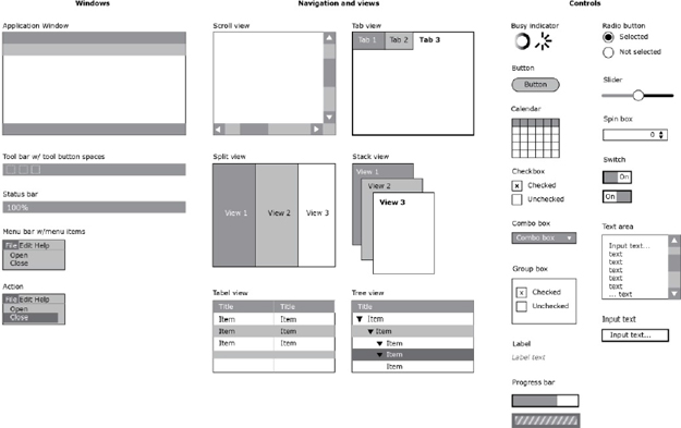
Figure 2.9. Different types of control widgets as they are rendered on the computer screen, inspired from Qt Quick Controls module. The graphic style has been simplified. It may actually change in different platforms
Table 2.7. HTML forms, input types, jQuery UI widgets and interaction methods
| HTML form tags | HTML input tag types | jQuery UI widgets | jQuery UI interaction |
| <form>, <input>, <textarea>, <button>, <select>, <optgroup>, <option>, <label>, <fieldset>, <legend>, <datalist>, <keygen>, <output> | button, checkbox, color, date, datetime-local, email, file, hidden, image, month, number, password, radio, range, reset, search, submit, tel, text, time, url, week | Accordion, Autocomplete, Button, Checkboxradio, Controlgroup, Datepicker, Dialog, Menu, Progressbar, Selectmenu, Slider, Spinner, Tabs, Tooltip | Draggable, Droppable, Resizable, Selectable, Sortable, |
2.3.2.3. Graphical interface models, structures, patterns
While the semantics of GUI elements is discovered through direct manipulation (pressing, releasing, dragging, stretching, launching actions, etc.), it is also recommended to satisfy a user’s model and to fulfill the expected user’s experiences. A user’s model approach implies designing in terms of needs and usefulness. From this strand, developing a GUI requires to have a clear idea of the following questions: what is its purpose (what can we do, how can it help to do something)? What is the profile of a typical user (background, domain, language, age)?
Throughout the evolution of user interfaces, various approaches have placed special interest on how GUI elements will be organized. One of the most famous initiatives has been the Apple Human Interface Guidelines, initiated in 1987 and still in use today for designing desktop applications using the Mac environment and tools38. In a similar manner, Google introduced in 2015 its own view called Material Design including guidelines and a vast gallery of resources39.
In a broader sense, computer scientist Siegfried Treu proposed the term interface structures to signify organizational and relational patterns among GUI elements. Inspired by the same logic behind object-oriented programming and taking into account research from cognitive sciences, Treu considered three types of representations: propositional (objects, ideas, symbols, words), analogical (dimensions, shapes, sizes) and procedural (instructions, actions, lists, sets) [TRE 94, p. 60]. He identified seven patterns or structures:
- – Object-oriented structures: objects are explicitly linked as networks of nodes;
- – Set structures: elements are grouped together according to some criteria;
- – Horizontal and vertical structures: elements follow hierarchical or sequential organizations;
- – Spatial structures: elements float around the visible space at any position (this pattern can be extended to volumes in 3D);
- – Context-providing structures: central elements are enveloped or surrounded by other elements at determinate distance;
- – Language structures: elements react to each other in a conversational or action–reaction sequence.
More recently, the notion of user interface has broadened with the variety of platforms, devices and software applications. In fact, interface models are no longer limited to considering widgets as the basic interface elements, but also the spatial configurations of visual components. Following interface designer Jenifer Tidwell, what we observe today are interface idioms (prototypical styles of a kind of interface: it is in these terms that we speak about word processor interfaces, paint interfaces, or spreadsheet interfaces) and “a loosening of the rules for putting together interfaces from these idioms” [TID 11, p. xvi]. In this respect, Tidwell also identifies patterns from a wide variety of domains. More precisely, she identifies 101 patterns or best practices organized in nine categories (see Table 2.8): navigation, layout, lists, actions and commands, trees and charts, forms and controls, social media, mobile devices, and visual style.
Table 2.8. Interface patterns, from [TID 11]
| Navigation | Clear entry points; menu page; pyramid (tree); modal panel; deep-linked state; escape hatch; fat menus; sitemap footer; sign-in tools; sequence map; breadcrumbs; annotated scrollbar; animated transition |
| Layout | Visual framework; center stage; grid of equals; titled sections; module tabs; accordion; collapsible panels; movable panels; right/left alignment; diagonal balance; responsive disclosure; responsive enabling; liquid layout |
| Lists | Two-panel selector; one-window drilldown; list inlay; thumbnail grid; carousel; row striping; pagination; jump to item; alphabet scroller; cascading lists; tree table; new-item row |
| Actions and commands | Button groups; hover tools; action panel; prominent “done” button; smart menu items; preview; progress indicator; cancelability; multi-level undo; command history; macros |
| Trees and charts | Overview plus detail; datatips; data spotlight; dynamic queries; data brushing; local zooming; sortable table; radial table; multi-y graph; small multiples; treemap |
| Forms and controls | Forgiving format; structured format; fill-in-the-blanks; input hints; input prompt; password strength meter; autocompletion; dropdown chooser; list builder; good defaults; same-page error messages |
| Social media | Editorial mix; personal voices; repost and comment; conversation starters; inverted nano-pyramid; timing strategy; specialized streams; social links; sharing widget; news box; content leaderboard; recent chatter |
| Mobile devices | Vertical stack; filmstrip; touch tools; bottom navigation; thumbnail-and-text list; infinite list; generous borders; text clear button; loading indicators; richly connected apps; streamlined branding |
| Visual style | Deep background; few hues, many values; corner treatments; borders that echo fonts; hairlines; contrasting font weights; skins and themes |
To conclude this part, we will discuss how graphical interfaces also consist of linkage structures, that is, the web of links between the visual components. Within the domain of hypertext and hypermedia, this approach is broadly studied as rhetoric of hypertext: how information is written and read through user interfaces. Computer scientist Mark Bernstein, in his seminal article [BER 98] identifies different patterns of hypertext:
- – Cycles: the structure of a text is recognized by returning over an entry point and departing towards a new path. This can be experienced when returning to the same home page in websites. When several web pages or entire hypertexts are linked together, the cycle can be known as a web ring.
- – Mirrorworlds: two or more different sets of nodes are put together in order to favor comparison. The structure is recognized implicitly by the reader, who identifies different parallel statements.
- – Tangle: links do not explicitly help the reader to distinguish the destination or action that will occur upon making a choice. This structure makes the reader aware of the existence of new and unknown information.
- – Sieves: these are tree-like structures representing layers of choice and organization.
- – Montage: various spaces appear together, maybe overlapping or freely floating around a larger space. Spaces can be distinguished from each other, and also each space has its own information and identity.
- – Neighborhood: similar to the context-providing structures in [TRE 94]; nodes emphasize the associative structure of texts by visual properties and proximity.
- – Missing links or nodes: the structure is suggested by explicit missing elements (like a blank space among list items) or suggested links, using rhetorical figures like allusion or narrative techniques like ellipsis.
- – Feint: shows the diverse entry points or the overall parts of a text. It might provide access to individual parts and, more importantly, it creates the structure of possibilities that can be navigated further after.
Although these patterns have been observed for creative writing purposes in spatial hypertext systems, they are also found in the design of multipurpose systems. Systems such as Tinderbox exploit visual attributes of nodes and links, and also provide an environment to express structure through several spatial models [BER 12a]. This is also the case in visual or associative programming software like Pure Data or Max/MSP devoted to audio signal processing (the next chapter discusses examples in more detail).
2.3.3. Image file formats
Image file formats refer to the stored representation of visual information. Commonly, we identify two types of formats, vector and bitmap formats, and both handle information in a sequential alphanumeric manner.
2.3.3.1. Vector formats
Although the name vector format derives historically from images specifically created for vector displays (also known as random-scan systems such as oscilloscopes monitors), they have been eventually replaced by raster-scan systems. Nevertheless, vector formats are recurrent in literature and denote an image representation in terms of geometric information.
We have already mentioned the SVG graphics language in section 2.3.1. The syntax and structure of SVG is defined in an XML namespace. Accordingly, an SVG image is composed of a sequence of tags and attributes in a text form. Another format based on XML is COLLADA, introduced in 1982 and currently maintained by the Khronos Group. COLLADA is a format dedicated to 3D graphics. One of its goals is to facilitate the exchange of assets (or models) between software applications. The current version is 1.5 (specified in 2008) and supports graphics defined with OpenGL ES 2.040.
Some vector formats support different representations, either as ASCII or as binary code. In the first case, the visual information is described with only ASCII characters, meanwhile the binary form relies on series of bits and algorithms to make the reading and writing of large files more efficient. A binary file would often be preferred if the file size is a constraint. Examples of formats that support both configurations are: DXF (acronym of Drawing Exchange Format) developed for Autodesk AutoCAD in 1982, and STL (acronym of Stereolithography), introduced in 1987 by 3D systems (a pioneer company in 3D printing systems).
Table 2.9. Data keywords in the OBJ file format41
| Vertex data | Elements | Free-form curve/surface attributes |
| v: geometric vertices v vt: texture vertices vn: vertex normals vp: parameter space vertices |
p: point l: line f: face curv: curve curv2: 2D curve surf: surface |
cstype: rational or non-rational forms of curve or surface type: basis matrix, Bezier, B-spline, Cardinal, Taylor deg: degree bmat: basis matrix step: step size |
| Free-form curve/surface body statements | Grouping and Connectivity between free-form surfaces | Display/render attributes |
| parm: Parameter values trim: outer trimming loop hole: inner trimming loop scrv: special curve sp: special point end: end statement |
g: group name s: smoothing group mg: merging group o: object name con: connect |
bevel: bevel interpolation c_interp: color interpolation d_interp: dissolve interpolation lod: level of detail usemtl: material name mtllib: material library shadow_obj: shadow casting trace_obj: ray tracing ctech: curve approximation stech: surface approximation |
One of the most used formats is OBJ, developed in 1992 by Wavefront Technologies (later merged with Alias and later acquired by Autodesk) and available as an open format. OBJ offers a clear specification to exemplify the structure of data inside a file. It determines seven classes; each one identified with a specific keyword. Once a model or surface has been generated and exported to OBJ, the file contains a series of lines referring to the data keywords and their values.
2.3.3.2. Raster file formats
Raster file formats are the most common image file formats today. They can be seen as a direct interface between the visual information and the screen monitor. Indeed, for graphics systems, the color screen is represented as a series of RGB values. These values are stored in the frame buffer, which is refreshed continuously (typically at the rate of 60 Mhz). The RGB values are stored as non-negative integers and the range of values depends on the number of bits per pixel position. As we said earlier, in true color images, each pixel has three color components (red, blue and green), each of 8 bits. If we recall the binary conversions in Table 2.3, the maximum values that one component allocates is 256 (or 255 if we start to count from 0). Anecdotally, the term bitmap image was referred originally to monochrome images, while pixmap was used for multiple bits per pixel. However, the name bitmap is used indistinctly to signify raster images [HEA 04, p. 779].
In raster images, the visual information is structured in a binary form, and it might include additional information such as metadata, look-up tables, or compression types. Moreover, some formats may act as containers or metafiles (i.e. a format like PDF can contain JPEG images). Examples of raster formats are BMP, GIF, PNG and JPEG, among hundreds of others. Here, we briefly describe them.
BMP (or simply bitmap) was one of the earliest image formats, introduced by Microsoft for applications like Paint and Paintbrush in 1985. The structure of a .bmp consists of a header part (which uses 14 bytes of memory for specifying types, size and layout); the bitmap information part (which uses 40 bytes and specifies dimensions, compression type, and color format); and the bitmap data, consisting of values representing rows of the image in left-to-right order.
GIF (Graphics Interchange Format) was developed in 1987 by UNYSIS and CompuServe. It initiated as an adapted format for electronic transmission. In 1989, the format was modified to support animation (animated GIFs), which has propelled its popularity among online social networks in recent years. The file structure has five parts: the signature, the screen descriptor, the color map, the image descriptor, and the GIF terminator.
PNG (Portable Network Graphics) started as an open alternative to GIF license fees. Its first specification was published in 1996 (four years after JPEG). Among other features of PNG, we highlight the support to 48-bit images, which allow the addition of transparency layers into 24-bit color images, as well as color correction information. The structure of PNG files is given in the form of block chunks (using the PNG jargon). There are different kinds of chunks: critical, public, private, and safe-to-copy. We note that PNG files can be extended with additional metadata, such as the XMP recommendation: physically, this information goes inside the text block iTXt, with the identifier XML:com.adobe.xmp.
JPEG (Joint Photographic Experts Group) was first published in 1992 and standardized by ISO/IEC 10918-1. JPEG actually covers a variety of specifications regarding digital images: first, the coding technology; second, the compliance testing; and third, the extensions and format. As a matter of fact, it is this third part, the JFIF (JPEG File Interchange Format) which is generally referred as the JPEG file format. These specifications are not freely available.
JPEG has become the most popular format because of its great compression rate. There are actually four compression methods: lossless, sequential, progressive and hierarchical. The first two modes are almost the only ones used; they are known as Huffman-encoded with 8-bit samples. The lossless has been superseded by other standards and the hierarchical bares the barrier of its complexity. When we refer to sampling, this is the first step in the JPEG encoding scheme. Sampling implies converting RGB colors into YCbCr color space. Y stands for luminance (it is a black and white representation of the image), Cb for the blueness of the image, and Cr for its redness. After sampling, the image is compressed into data units (8 x 8 pixel blocks). The technique uses operations in the frequency domain, a DCT (discrete cosine transform) to store data as cosine functions. The third step is quantization, where non-essential cosine functions are eliminated in order to recreate the original. The last step is the Hoffman coding, where only quantized DCT coefficients are encoded.
The structure of a JPEG file is decomposed by means of markers. There are 2 bytes per marker: the first part is always FF values and the second part denotes the code of the market type. A typical structure is:
Before closing this part, it is important to recall one last format technique heavily used in web environments via the HTML5 canvas element. Base 64 is a base encoding of data used in situations where only ASCII characters are allowed (e.g. a URL name address). It is constructed from a subset of 64 characters42: letters from A to Z (uppercase), a to z (lowercase), numbers from 0 to 9, underscore and minus sign. The 65th character (equal sign) is dedicated to represent processing functions. Among its implementations, the HTML5 canvas method toDataURL() can be used to generate compressed images and to distribute them directly in the URL bar of web browsers. The identifier starts with the protocol and instruction: data:image/png;base64.
| Values | Symbol used by JPEG | Description |
| FFD8 | SOI | Start of image |
| FFE0-FFEF | APP | Application-specific data or associated information. It is in this part that metadata like EXIF and XMP is added |
| FFC4 | DHT | Define Huffman Table |
| FFDB | DQT | Define Quantization Table |
| FFCD | SOF | Start of frame. In JPEG terminology, a frame is the equivalent of a picture |
| Second tables: DHT or DQT | ||
| FFDA | SOS | Start of scan. A scan is a pass through the pixel color values; a segment is a group of blocks, and a block is a series of 8 x 8 pixels |
| Scan Data 1 | This is the only part of a JPEG file that does not happen within a marker; however, it always follows an SOS marker | |
| N tables: DHT or DQT N SOS: start of scan n times Scan Data n times |
||
| FFD9 | EOI | End of image |
2.4. Objectual materiality of visual information
The third level of our trajectory depicted in Table 2.1 focuses on the materialization and effects of computing, as it is perceptible in the physical world through our senses. The inscription devices that we explored in the last section (GUIs, programming languages, file formats) participate now as formal supports of image interfaces. That means the technical, material and corporal characteristics of the screen and other devices are determined and configured to respond to them. However, this is also a dialectic process. While hardware is built on top of other levels of computing, it can also modify those levels (following a downward direction in the trajectory, innovating new algorithms, new data structures, new data types).
From the perspective of visual information and visual interfaces, we often talk about graphics systems as complex apparatuses that combine CPU (central processing units), GPU (graphics processing unit), screens, and interaction devices (mouse, keyboard, etc.) The most important material support for our study will be the computer screen. But, more broadly, we will focus on the relationship between materials and visual information: how they handle it, how are they are conceived to communicate with each other. Hence, we will also take a look at capturing devices (sensors, lenses) and printing devices (both 2D and 3D).
2.4.1. Screen
Images appear on screen following the canonical raster display model. This is also true for video projectors, touch screens, and as we will see later, for capturing and printing devices. The overall idea is that the surface display is represented as a rectangular grid of screen pixels, each one of these directly associated with the image samples (the fundamental pixel values that constitute the digital image). In the raster scan model, an electron beam sweeps across the screen, left-to-right and top-to-bottom43, varying its intensity at each screen pixel position. Rows are named scan lines and the total screen area is called a frame. The representation of one state of the screen is saved in the frame buffer.
A digital image described as pixel values (0 for black and 255 for white) has its corresponding visual representation in a raster grid. Rectangular grids are by far the most common types of sampling grids44. To simplify, we show in Figure 2.10 a 5 × 5 grid and, in Figure 2.11, logical operations, AND, NOT, XOR, performed on rectangular grids. These operations are applied from the new incoming values (source) to those already stored in the frame buffer (destination).

Figure 2.10. Common types of grids

Figure 2.11. Logical operations (transfer modes)
In current display systems, there are several properties that can be identified:
- – Resolution: the amount of screen pixels to be illuminated. Different resolutions depend on the aspect ratio, but screens have evolved from 640 × 480 (4:3 ratio) in the 1990s to the more recent 1920 × 1080 (16:9 ratio) in the 2010s.
- – Aspect ratio: the relation given between the number of screen pixel columns divided by the number of scan lines that can be displayed. Historically, screens have moved from square ratios (4:3) to more rectangular widescreen ratios (16:9).
- – Refresh rate: the amount of time at which the frame is rescanned. From film studies, we know that below 24 frames per second (fps), the human eye might detect gaps between images. Later, with the arrival of television and video, the rate used was 30 fps according to the time in which phosphor decays. In recent systems, frame cycles are measured in Hertz. Typically, we use 60 Hz because interlaced images require twice the time to sweep a frame (30 fps per pass), but higher cycles include 80 or 120 Hz.
- – Color: the common standard is the true color system, containing 24 bits per pixel in the frame buffer, “allowing 256 voltage settings for each electron gun, nearly 17 million color choices for each pixel” [HEA 04, p. 44].
Although the raster model initiated with cathode ray tube (CRT) display technologies, it remains valid in recent screen devices based on light-emitting diodes (LEDs) or liquid crystal displays (LCDs). While in CRT monitors, the screen pixels produce a glowing (“circular area containing an RGB triad of phosphors on the screen” [HUG 14, p. 20]), in LCD monitors, each screen pixel is a set of three rectangles corresponding to the red, green and blue spectra. Then, there is backlight behind the screen that is filtered by these rectangles. Even though there is a small space between color dots or stripes, they are not visible when the space is less than 200 micrometers, thus producing a continuous image [RUS 11, p. 55].
2.4.2. Cameras, sensors, lenses
Digital cameras are imaging systems composed of photosensitive sensors, a lens and electronic circuitry that digitizes the image. They are of course not the only system used for image acquisition. Given the variety of wavelengths in the electromagnetic spectrum (see section 1.1.1), there are multiple devices and components designed for different purposes (from microscopes to space probes). The example of digital cameras is worth noting because of their popularity, available in a wide range of devices.
The overall process for image acquisition through digital cameras is as follows. When visible light hits the lens, it projects the viewed scene to the sensors, which converts the light energy to voltages. Then, electronic circuitry transforms the output into analog and digital signals, resulting in a 2D digital image. Let’s now analyze in more detail each component in relation to visual information.
The physical quantity measured by lenses is irradiance, also referred to as brightness or intensity. In order to match the projected scene, the ultimate goal is to make a straight ray correspond directly from the scene to the sensor (this is also called the pinhole model). In practice, this is not the case because lenses introduce optics aberrations that need to be handled in software. The five main types of aberrations are: spherical distortion, coma, astigmatism, curvature of field, and color aberration [SON 08, pp. 86–87]. Curvature of field includes geometric distortions such as barrel (dispersion away from the observed scene) and pincushion effects (dispersion towards the image center). Another example of distortion is vignetting, caused by the loss of visual information at the edges of the image boundaries. Figure 2.12 shows barrel and pincushion effects as they are simulated and available through Nik Colleciton45, precisely the Analog Efex Pro 2→Lens distortion.
As we mentioned, photosensitive image sensors convert photons to electrical signals. Technically, sensors can be grouped according to two principles. On the one hand, those based on photo emission, as used in vacuum tube television cameras, and on the other hand, those based on photovoltaic principles, as used in the development of semiconductors. In this line, there have been two types applied to cameras: CCD (charged-coupled devices) and CMOS (complementary metal oxide semiconductor). The latter has become the de facto standard in devices requiring low power consumption (such as mobile devices). Sensors are commonly arranged in the form of a 2D array with an additional color filter to create a color camera. The most common filter pattern is the Bayer mosaic which assigns “twice as many detectors for green as for red or blue, which mimics to some extent the human eye’s greater sensitivity to green” [RUS 11, p. 17].

Figure 2.12. Barrel and pincushion effects in Nik Collection
At this level, it is interesting to note two things. First, the small capacity of CMOS chips results in lowering the brightness resolution of captured images. However, images are stored in 8-bit per channel anyway, to cope with the standard model. Second, it is the combination of color filter and the interpolation algorithms used in the camera that is used as a signature to identify the model or to check if any alteration has been made.
2.4.3. 2D and 3D printing devices
Printing implies moving an image beyond the screen into a rigid physical support. The technique to achieve this goal is also based on the raster grid model. In 2D, there are several kinds of printers, inks and papers that are used to obtain the desired result. Printing is based on two fundamental concepts: the density of dots and the pattern in which such dots are arranged.
Density of dots is also known as dpi (dots per inch). A general rule is that the lower the dpi, the lower the quality of images (characterized by a jagged or “pixelated” effect). To solve this issue, it is possible to increment the number of dpi in an image. A value of approximately 300 dpi is satisfactory for house and reports, but professional imaging material relies on 1200 dpi at least. The basic problem is that the computer screen is based on 72 dpi. Moreover, the type of ink and paper will also be important, as ink might spread and dry differently.
Dots produced by the printer are arranged through the halftone technique. This is necessary because the size and the intensity of dots cannot be modulated. Ideally, an image pixel can be represented as a halftone cell. For instance, a 4 × 4 array can group 16 dots with 17 possible gray levels (white being the absence of dots, given by the surface of the paper). In theory then, “if each pixel corresponds to a halftone cell, then an image can be printed with about the same dimension as it appears on the screen” [RUS 11, p. 143]. But if screen resolutions range from 72 to 100 dpi, it is necessary to preview with software the lack of physical space.
In the case of printing colors, there is a fundamental passage from the screen to paper. Printers are based on the subtractive color scheme (also known as CMYK), which starts from the white of the paper. Cyan, magenta and yellow are added in order to remove the complementary colors red, green and blue. The full color model includes a layer of black in order to conserve as much as possible the use of other inks and to obtain a more contrasting black tone. The way in which CMYK halftones dictates avoiding moiré patterns by rotating the CMYK rectangular layers by 45, 70, 90 and 105 degrees, respectively: “This aligns the colored screens to form small rosettes that together make up the color” [RUS 11, p. 154].
Regarding 3D printing, the process has been named more accurately as additive manufacturing. It is additive because the techniques involve adding layers of raw material to form a solid object. And it is more related to manufacturing because of the complexity and delicateness of materials: sometimes the expected result fails; sometimes the material needs special handling (masks, gloves).
The first era of 3D printers occurred during the 1980s, but it was not until the year 2005 that 3D printing received serious attention, thanks in large extent to the “maker” and DIY (do it yourself) movements. We can identify two main types of 3D printers:
- – Selection deposition printers: this is one of the pioneering and also safest printers, available in early models for home, office and schools. The main characteristic is they “squirt, spray, or squeeze liquid, paste, or powdered raw material through some kind of syringe or nozzle”. The principal raw material is plastic, which hardens once printed.
- – Selective binding printers: these printers use light or lasers to solidify two main kinds of materials. On the one hand, a light sensitive photopolymer is used in stereolitography (SL), in which: “The printer sweeps a laser beam over the surface of a special type of plastic, a UV-sensitive photopolymer that hardens when exposed to UV light. Each sweep of the laser traces the outline and cross-section of the printed shape in consecutive layers” [LIP 13, p. 73]. On the other hand, laser sintering (SL) uses a similar process, but uses powder instead of liquid photopolymers.
In any case, just as 2D image files have a direct relationship with the printed version, the same holds true for 3D. A file format like STL organizes the geometric information (in triangles and polygons) that will be interpreted as “slices” or virtual layers by the printer firmware.