
7 Understanding Java performance
- Why performance matters
- The G1 garbage collector
- Just-in-time (JIT) compilation
- JFR—the JDK Flight Recorder
Poor performance kills applications—it’s bad for your customers and your application’s reputation. Unless you have a totally captive market, your customers will vote with their feet—they’ll already be out the door, heading to a competitor. To stop poor performance from harming your project, you need to understand performance analysis and how to make it work for you.
Performance analysis and tuning is a huge subject, and too many treatments focus on the wrong things. So, we’re going to start by telling you the big secret of performance tuning. Here it is—the single biggest secret of performance tuning: You have to measure. You can’t tune properly without measuring.
And here’s why: the human brain is pretty much always wrong when it comes to guessing what the slow parts of systems are. Everyone’s is. Yours, mine, James Gosling’s—we’re all subject to our subconscious biases and tend to see patterns that may not be there. In fact, the answer to the question, “Which part of my Java code needs optimizing?” is quite often, “None of it.”
Consider a typical (if rather conservative) ecommerce web application, providing services to a pool of registered customers. It has an SQL database, web servers fronting Java services, and a fairly standard network configuration connecting all of it. Very often, the non-Java parts of the system (database, filesystem, network) are the real bottleneck, but without measurement, the Java developer would never know that. Instead of finding and fixing the real problem, the developer may waste time on micro-optimization of code aspects that aren’t really contributing to the issue.
The kinds of fundamental questions that you want to be able to answer are these:
-
If you have a sales drive and suddenly have 10 times as many customers, will the system have enough memory to cope?
-
What is the average response time your customers see from your application?
Notice that all of these example questions are about aspects of your system that are directly relevant to your customers—the users of your system. There is nothing here about topics such as
The inexperienced performance engineer will often make the mistake of assuming that user-visible performance is strongly dependent upon, or closely correlated with, the microperformance aspects that the second set of questions addresses.
This assumption—essentially a reductionist viewpoint—is actually not true in practice. Instead, the complexity of modern software systems causes overall performance to be an emergent property of the system and all of its layers. Specific microeffects are almost impossible to isolate, and microbenchmarking is of very limited utility to most application programmers.
Instead, to do performance tuning, you have to get out of the realm of guessing about what’s making the system slow—and slow means “impacting the experience of customers.” You have to start knowing, and the only way to know for sure is to measure.
You also need to understand what else performance tuning isn’t. It isn’t the following:
Be especially careful of the “tips and tricks” approaches. The truth is that the JVM is a very sophisticated and highly tuned environment, and without proper context, most of these tips are useless (and may actually be harmful). They also go out of date very quickly as the JVM gets smarter and smarter at optimizing code.
Performance analysis is really a type of experimental science. You can think of your code as a type of science experiment that has inputs and produces “outputs”—performance metrics that indicate how efficiently the system is performing the work asked of it. The job of the performance engineer is to study these outputs and look for patterns. This makes performance tuning a branch of applied statistics, rather than a collection of old wives’ tales and applied folklore.
This chapter is here to help you get started. It’s an introduction to the practice of Java performance tuning. But this is a big subject, and we have space to give you only a primer on some essential theory and some signposts. We’ll try to answer the following most fundamental questions:
-
What aspects of the JVM make it potentially complex to tune?
-
How should performance tuning be thought about and approached?
We’ll also give you an introduction to the following two subsystems in the JVM that are the most important when it comes to performance-related matters:
This should be enough to get you started and help you apply this (admittedly somewhat theory-heavy) knowledge to the real problems you face in your code. Let’s get going by taking a quick look at some fundamental vocabulary that will enable you to express and frame your performance problems and goals.
7.1 Performance terminology: Some basic definitions
To get the most out of our discussions in this chapter, we need to formalize some notions of performance that you may be aware of. We’ll begin by defining some of the following important terms in the performance engineer’s lexicon:
A number of these terms are discussed by Doug Lea in the context of multithreaded code, but we’re considering a much wider context here. When we speak of performance, we could mean anything from a single multithreaded process all the way up to an entire cluster of services hosted in the cloud.
7.1.1 Latency
Latency is the end-to-end time taken to process a single work unit at a given workload. Quite often, latency is quoted just for “normal” workloads, but an often-useful performance measure is the graph showing latency as a function of increasing workload.
The graph in figure 7.1 shows a sudden, nonlinear degradation of a performance metric (e.g., latency) as the workload increases. This is usually called a performance elbow (or “hockey stick”).

7.1.2 Throughput
Throughput is the number of units of work that a system can perform in some time period with given resources. One commonly quoted number is transactions per second on some reference platform (e.g., a specific brand of server with specified hardware, OS, and software stack).
7.1.3 Utilization
Utilization represents the percentage of available resources that are being used to handle work units, instead of housekeeping tasks (or just being idle). People will commonly quote a server as being, for example, 10% utilized. This refers to the percentage of CPU processing work units during normal processing time. Note that the difference can be very large between the utilization levels of different resources, such as CPU and memory.
7.1.4 Efficiency
The efficiency of a system is equal to the throughput divided by the resources used. A system that requires more resources to produce the same throughput is less efficient.
For example, consider comparing two clustering solutions. If solution A requires twice as many servers as solution B for the same throughput, it’s half as efficient.
Remember that resources can also be considered in cost terms—if solution A costs twice as much (or requires twice as many staff to run the production environment) as solution B, then it’s only half as efficient.
7.1.5 Capacity
Capacity is the number of work units (such as transactions) that can be in flight through the system at any time. That is, it’s the amount of simultaneous processing available at a specified latency or throughput.
7.1.6 Scalability
As resources are added to a system, the throughput (or latency) will change. This change in throughput or latency is the scalability of the system.
If solution A doubles its throughput when the available servers in a pool are doubled, it’s scaling in a perfectly linear fashion. Perfect linear scaling is very, very difficult to achieve under most circumstances—remember Amdahl’s law.
You should also note that the scalability of a system depends on a number of factors, and it isn’t constant. A system can scale close to linearly up until some point and then begin to degrade badly. That’s a different kind of performance elbow.
7.1.7 Degradation
If you add more work units, or clients for network systems, without adding more resources, you’ll typically see a change in the observed latency or throughput. This change is the degradation of the system under additional load.
The degradation will, under normal circumstances, be negative. That is, adding work units to a system will cause a negative effect on performance (such as causing the latency of processing to increase). But some circumstances exist under which degradation could be positive. For example, if the additional load causes some part of the system to cross a threshold and switch to a high-performance mode, this can cause the system to work more efficiently and reduce processing times, even though there is actually more work to be done. The JVM is a very dynamic runtime system, and several parts of it could contribute to this sort of effect.
The preceding terms are the most frequently used indicators of performance. Others are occasionally important, but these are the basic system statistics that will normally be used to guide performance tuning. In the next section, we’ll lay out an approach that is grounded in close attention to these numbers and that is as quantitative as possible.
7.2 A pragmatic approach to performance analysis
Many developers, when they approach the task of performance analysis, don’t start with a clear picture of what they want to achieve by doing the analysis. A vague sense that the code “ought to run faster” is often all that developers or managers have when the work begins.
But this is completely backward. To do really effective performance tuning, you should have think about some key areas before beginning any kind of technical work. You should know the following things:
-
How you’ll recognize when you’re done with performance tuning
-
What the maximum acceptable cost is (in terms of developer time invested and additional complexity in the code) for the performance tuning
Most important, as we’ll say many times in this chapter, you have to measure. Without measurement of at least one observable, you aren’t doing performance analysis.
It’s also very common when you start measuring your code to discover that time isn’t being spent where you think it is. A missing database index or contended filesystem locks can be the root of a lot of performance problems. When thinking about optimizing your code, you should always remember that it’s possible that the code isn’t the issue. To quantify where the problem is, the first thing you need to know is what you’re measuring.
7.2.1 Know what you’re measuring
In performance tuning, you always have to be measuring something. If you aren’t measuring an observable, you’re not doing performance tuning. Sitting and staring at your code, hoping that a faster way to solve the problem will strike you, isn’t performance analysis.
Tip To be a good performance engineer, you should understand terms such as mean, median, mode, variance, percentile, standard deviation, sample size, and normal distribution. If you aren’t familiar with these concepts, you should start with a quick web search and do further reading if needed. Chapter 5 of Leonard Apeltsin’s Data Science Bookcamp (Manning, 2021. http://mng.bz/e7Oq) is a good place to start.
When undertaking performance analysis, it’s important to know exactly which of the observables we described in the last section are important to you. You should always tie your measurements, objectives, and conclusions to one or more of the basic observables we introduced. Some typical observables that are good targets for performance tuning follow:
-
Average time taken for the
handleRequest()method to run (after warmup) -
The 90th percentile of the system’s end-to-end latency with 10 concurrent clients
-
The degradation of the response time as you increase from 1 to 1,000 concurrent users
All of these represent quantities that the engineer might want to measure and potentially tune. To obtain accurate and useful numbers, a basic knowledge of statistics is essential.
Knowing what you’re measuring and having confidence that your numbers are accurate is the first step. But vague or open-ended objectives don’t often produce good results, and performance tuning is no exception. Instead, your performance goals should be what are sometimes referred to as SMART objectives (for specific, measurable, agreed, relevant, and time-boxed).
7.2.2 Know how to take measurements
We have really only the following two ways to determine precisely how long a method or other piece of Java code takes to run:
-
Measure it directly, by inserting measurement code into the source class.
-
Transform the class that is to be measured at class loading time.
These two approaches are referred to as manual and automatic instrumentation, respectively. All commonly used performance measuring techniques will rely on one (or both) of these techniques.
Note There is also the JVM Tool Interface (JVMTI), which can be used to create very sophisticated performance tools, but it has drawbacks, notably that it requires the use of native code, which impacts both the complexity and safety of tools written using it.
Direct measurement is the easiest technique to understand, but it’s also intrusive. In its simplest form, it looks like this:
long t0 = System.currentTimeMillis();
methodToBeMeasured();
long t1 = System.currentTimeMillis();

long elapsed = t1 - t0;
System.out.println("methodToBeMeasured took "+ elapsed +" millis");
This will produce an output line that should give a millisecond-accurate view of how long methodToBeMeasured() took to run. The inconvenient part is that code like this has to be added throughout the codebase, and as the number of measurements grows, it becomes difficult to avoid being swamped with data.
There are other problems too—for example, what happens if methodToBeMeasured() takes under a millisecond to run? As we’ll see later in this chapter, there are also cold-start effects to worry about: JIT compilation means that later runs of the method may well be quicker than earlier runs.
There are also more subtle problems: the call to currentTimeMillis() requires a call to a native method and a system call to read the system clock. This is not only time-consuming but can also flush code from the execution pipelines, leading to additional performance degradation that would not occur if the measurement code was not there.
Automatic instrumentation via class loading
In chapters 1 and 4, we discussed how classes are assembled into an executing program. One of the key steps that is often overlooked is the transformation of bytecode as it’s loaded. This is incredibly powerful, and it lies at the heart of many modern techniques in the Java platform.
One example of it is the automatic instrumentation of methods. In this approach, methodToBeMeasured() is loaded by a special class loader that adds in bytecode at the start and end of the method to record the times at which the method was entered and exited. These timings are typically written to a shared data structure, which is accessed by other threads. These threads act on the data, typically either writing output to log files or contacting a network-based server that processes the raw data.
This technique lies at the heart of many professional-grade Java performance-monitoring tools (such as New Relic), but actively maintained open source tools that fill the same niche have been scarce. This situation may now be changing with the rise of the OpenTelemetry OSS libraries and standards and their Java auto-instrumentation subproject.
Note As we’ll discuss later, Java methods start off interpreted, then switch to compiled mode. For true performance numbers, you have to discard the timings generated when in interpreted mode, because they can badly skew the results. Later we’ll discuss in more detail how you can know when a method has switched to compiled mode.
Using one or both of these techniques will allow you to produce numbers for how quickly a given method executes. The next question is, what do you want the numbers to look like when you’ve finished tuning?
7.2.3 Know what your performance goals are
Nothing focuses the mind like a clear target, so just as important as knowing what to measure is knowing and communicating the end goal of tuning. In most cases, this should be a simple and precisely stated goal, such as the following:
In more complex cases, the goal may be to reach several related performance targets at once. You should be aware that the more separate observables that you measure and try to tune, the more complex the performance exercise can become. Optimizing for one performance goal can negatively impact on another.
Sometimes it’s necessary to do some initial analysis, such as determining what the important methods are, before setting goals, such as making them run faster. This is fine, but after the initial exploration, it’s almost always better to stop and state your goals before trying to achieve them. Too often developers will plow on with the analysis without stopping to elucidate their goals.
7.2.4 Know when to stop
In theory, knowing when it’s time to stop optimizing is easy—you’re done when you’ve achieved your goals. In practice, however, it’s easy to get sucked into performance tuning. If things go well, the temptation to keep pushing and do even better can be very strong. Alternatively, if you’re struggling to reach your goal, it’s hard to keep from trying out different strategies in an attempt to hit the target.
Knowing when to stop involves having an awareness of your goals but also a sense of what they’re worth. Getting 90% of the way to a performance goal can often be enough, and the engineer’s time may well be spent better elsewhere.
Another important consideration is how much effort is being spent on rarely used code paths. Optimizing code that accounts for 1% or less of the program’s runtime is almost always a waste of time, yet a surprising number of developers will engage in this behavior.
Here’s a set of very simple guidelines for knowing what to optimize. You may need to adapt these for your particular circumstances, but they work well for a wide range of situations:
-
Hit the most important (usually the most often called) methods first.
-
Take low-hanging fruit as you come across it, but be aware of how often the code that it represents is called.
At the end, do another round of measurement. If you haven’t hit your performance goals, take stock. Look and see how close you are to hitting those goals, and whether the gains you’ve made have had the desired impact on overall performance.
7.2.5 Know the cost of achieving higher performance
All performance tweaks have a price tag attached, such as the following:
-
There’s the time taken to do the analysis and develop an improvement (and it’s worth remembering that the cost of developer time is almost always the greatest expense on any software project).
-
There’s the additional technical complexity that the fix will probably have introduced. (There are performance improvements that also simplify the code, but they’re not the majority of cases.)
-
Additional threads may have been introduced to perform auxiliary tasks to allow the main processing threads to go faster, and these threads may have unforeseen effects on the overall system at higher loads.
Whatever the price tag, pay attention to it, and try to identify it before you finish a round of optimization.
It often helps to have some idea of what the maximum acceptable cost for higher performance is. This can be set as a time constraint on the developers doing the tuning, or as numbers of additional classes or lines of code. For example, a developer could decide that no more than a week should be spent optimizing, or that the optimized classes should not grow by more than 100% (double their original size).
7.2.6 Know the dangers of premature optimization
One of the most famous quotes on optimization is from Donald Knuth (“Structured Programming with go to Statements,” Computing Surveys, 6, no. 4 [December 1974].):
Programmers waste enormous amounts of time thinking about, or worrying about, the speed of noncritical parts of their programs, and these attempts at efficiency actually have a strong negative impact ... premature optimization is the root of all evil.
This statement has been widely debated in the community, and in many cases, only the second part is remembered. This is unfortunate for several reasons:
-
In the first part of the quote, Knuth is reminding us implicitly of the need to measure, without which we can’t determine the critical parts of programs.
-
We need to remember yet again that it might not be the code that’s causing the latency—it could be something else in the environment.
-
In the full quote, it’s easy to see that Knuth is talking about optimization that forms a conscious, concerted effort.
-
The shorter form of the quote leads to the quote being used as a fairly pat excuse for poor design or execution choices.
Some optimizations, in particular, the following, are really a part of good style:
In the following snippet, we’ve added a check to see if the logging object will do anything with a debug log message. This kind of check is called a loggability guard. If the logging subsystem isn’t set up for debug logs, this code will never construct the log message, saving the cost of the call to currentTimeMillis() and the construction of the StringBuilder object used for the log message:
But if the debug log message is truly useless, we can save a couple of processor cycles (the cost of the loggability guard) by removing the code altogether. This cost is trivial and will get lost in the noise of the rest of the performance profile, but if it genuinely isn’t needed, take it out.
One aspect of performance tuning is to write good, well-performing code in the first place. Gaining a better awareness of the platform and how it behaves under the hood (e.g., understanding the implicit object allocations that come from the concatenation of two strings) and thinking about aspects of performance as you go lead to better code.
We now have some basic vocabulary we can use to frame our performance problems and goals and an outline approach for how to tackle problems. But we still haven’t explained why this is a software engineer’s problem and where this need came from. To understand this, we need to delve briefly into the world of hardware.
7.3 What went wrong? Why do we have to care?
For a few halcyon years up until the mid-2000s, it seemed as though performance was not really a concern. Clock speeds were going up and up, and it seemed that all software engineers had to do was to wait a few months, and the improved CPU speeds would give an uptick to even badly written code.
How, then, did things go so wrong? Why are clock speeds not improving that much anymore? More worryingly, why does a computer with a 3 GHz chip not seem much faster than one with a 2 GHz chip? Where has this trend for software engineers across the industry to be concerned about performance come from?
In this section, we’ll talk about the forces driving this trend, and why even the purest of software developers needs to care a bit about hardware. We’ll set the stage for the topics in the rest of the chapter and give you the concepts you’ll need to really understand JIT compilation and some of our in-depth examples.
You may have heard the term “Moore’s law” bandied about. Many developers are aware that it has something to do with the rate at which computers get faster but are vague on the details. Let’s get under way by explaining exactly what it means and what the consequences are of it possibly coming to an end in the near future.
7.3.1 Moore’s law
Moore’s law is named for Gordon Moore, one of the founders of Intel. Here is one of the most common formulations of his law: The maximum number of transistors on a chip that is economic to produce roughly doubles every two years.
The law, which is really an observation about trends in computer processors (CPUs), is based on a paper he wrote in 1965, in which he originally forecast for 10 years—that is, up until 1975. That it has lasted so well is truly remarkable.
In figure 7.2 we’ve plotted a number of real CPUs from various families (primarily Intel x86 family) all the way from 1980 through to the latest (2021) Apple Silicon (graph data is from Wikipedia, lightly edited for clarity). The graph shows the transistor counts of the chips against their release dates.

This is a log-linear graph, so each increment on the y-axis is 10 times the previous one. As you can see, the line is essentially straight and takes about six or seven years to cross each vertical level. This demonstrates Moore’s law, because taking six or seven years to increase tenfold is the same as roughly doubling every two years.
Keep in mind that the y-axis on the graph is a log scale—this means that a mainstream Intel chip produced in 2005 had around 100 million transistors. This is 100 times as many as a chip produced in 1990.
It’s important to notice that Moore’s law specifically talks about transistor counts. This is the basic point that must be understood to grasp why Moore’s law alone isn’t enough for the software engineer to continue to obtain a free lunch from the hardware engineers (see Herb Sutter, “The Free Lunch Is Over: A Fundamental Turn Toward Concurrency in Software,” Dr. Dobb’s Journal 30 (2005): 202–210).
Moore’s law has been a good guide to the past, but it is formulated in terms of transistor counts, which is not really a good guide to the performance that developers should expect from their code. Reality, as we’ll see, is more complicated.
Note Transistor counts aren’t the same thing as clock speed, and even the still-common idea that a higher clock speed means better performance is a gross oversimplification.
The truth is that real-world performance depends on a number of factors, all of which are important. If we had to pick just one, however, it would be this: how fast can data relevant to the next instructions be located? This is such an important concept to performance that we should take an in-depth look at it.
7.3.2 Understanding the memory latency hierarchy
Computer processors require data to work on. If the data to process isn’t available, then it doesn’t matter how fast the CPU cycles—it just has to wait, performing no-operation (NOP) and basically stalling until the data is available.
This means that two of the most fundamental questions when addressing latency are, “Where is the nearest copy of the data that the CPU core needs to work on?” and “How long will it take to get to where the core can use it?” The main possibilities follow (in the so-called Von-Neumann architecture, which is the most commonly used form):
-
Registers—A memory location that’s on the CPU and ready for immediate use. This is the part of memory that instructions operate on directly.
-
Main memory—Usually DRAM. The access time for this is around 50 ns (but see later on for details about how processor caches are used to avoid this latency).
-
Solid-state drive (SSD)—It takes 0.1 ms or less to access these disks, but they’re still typically more expensive compared to traditional hard disks.
-
Hard disk—It takes around 5 ms to access the disk and load the required data into main memory.
Moore’s law has described an exponential increase in transistor count, and this has benefited memory as well—memory access speed has also increased exponentially. But the exponents for these two have not been the same. Memory speed has improved more slowly than CPUs have added transistors, which means there’s a risk that the processing cores will fall idle due to not having the relevant data on hand to process.
To solve this problem, caches—small amounts of faster memory (SRAM, rather than DRAM)—have been introduced between the registers and main memory. This faster memory costs a lot more than DRAM, both in terms of money and transistor budget, which is why computers don’t simply use SRAM for their entire memory.
Caches are referred to as L1 and L2 (some machines also have L3), with the numbers indicating how physically close to the core the cache is (closer caches will be faster). We’ll talk more about caches in section 7.6 (on JIT compilation) and show an example of how important the L1 cache effects are to running code. Figure 7.3 shows just how much faster L1 and L2 cache are than main memory.

As well as adding caches, another technique that was used extensively in the 1990s and early 2000s was to add increasingly complex processor features to try to work around the latency of memory. Sophisticated hardware techniques, such as instruction-level parallelism (ILP) and chip multithreading (CMT), were used to try to keep the CPU operating on data, even in the face of the widening gap between CPU capability and memory latency.
These techniques came to consume a large percentage of the transistor budget of the CPU, and the impact they had on real performance was subject to diminishing returns. This trend led to the viewpoint that the future of CPU design lay in chips with multiple (or many) cores. Modern processors are essentially all multicore—in fact, this is one of the second-order consequences of Moore’s law: core counts have gone up as a way to utilize available transistors.
The future of performance is intimately tied to concurrency—one of the main ways that a system can be made more performant overall is by utilizing more cores. That way, even if one core is waiting for data, the other cores may still be able to progress (but remember the impact of Amdahl’s law, which we introduced in chapter 5). This connection is so important that we’re going to say it again:
We’ve only scratched the surface of the world of computer architecture as it relates to software and Java programming. The interested reader who wants to know more should consult a specialist text, such as Computer Architecture: A Quantitative Approach, 6th edition, by Hennessy et al. (Morgan Kaufmann, December 2017).
These hardware concerns aren’t specific to Java programmers, but the managed nature of the JVM brings in some additional complexities. Let’s move on to take a look at these in the next section.
7.4 Why is Java performance tuning hard?
Tuning for performance on the JVM (or, indeed, any other managed runtime) is inherently more difficult than for code that runs unmanaged. In a managed system, the entire point is to allow the runtime to take some control of the environment, so that the developer doesn’t have to cope with every detail. This makes programmers much more productive overall, but it does mean that some control has to be given up.
This shift in emphasis makes the system as a whole harder to reason about because the managed runtime is an opaque box to the developer. The alternative is to give up all the advantages that a managed runtime brings, forcing programmers of, say, C/C++, to do almost everything for themselves. In this case, the OS supplies only minimal services, such as rudimentary thread scheduling, which is almost always a much higher overall time commitment than the additional effort required to performance tune.
Some of the most important aspects of the Java platform that contribute to making tuning hard follow:
These aspects can interact in subtle ways. For example, the compilation subsystem uses timers to decide which methods to compile. The set of methods that are candidates for compilation can be affected by concerns such as scheduling and GC. The methods that are compiled could be different from run to run.
As you’ve seen throughout this section, accurate measurement is key to the decision-making processes of performance analysis. An understanding of the details (and limitations) of how time is handled in the Java platform is, therefore, very useful if you want to get serious about performance tuning.
7.4.1 The role of time in performance tuning
Performance tuning requires you to understand how to interpret the measurements recorded during code execution, which means you also need to understand the limitations inherent in any measurement of time on the platform.
Quantities of time are usually quoted to the nearest unit on some scale. This is referred to as the precision of the measurement. For example, times are often measured to millisecond precision. A timing is precise if repeated measurements give a narrow spread around the same value.
Precision is a measure of the amount of random noise contained in a given measurement. We’ll assume that the measurements made of a particular piece of code are normally distributed. In that case, a common way of quoting the precision is to quote the width of the 95% confidence interval.
The accuracy of a measurement (in our case, of time) is the ability to obtain a value close to the true value. In reality, you won’t normally know the true value, so the accuracy may be harder to determine than the precision.
Accuracy measures the systematic error in a measurement. It’s possible to have accurate measurements that aren’t very precise (so the basic reading is sound, but random environmental noise exists). It’s also possible to have precise results that aren’t accurate.
An interval quoted at nanosecond precision as 5945 ns that came from a timer accurate to 1 μs is really somewhere between 3945–7945 ns (with 95% probability). Beware of performance numbers that seem overly precise; always check the precision and accuracy of the measurements.
The true granularity of the system is that of the frequency of the fastest timer—likely the interrupt timer, in the 10 ns range. This is sometimes called the distinguishability, the shortest interval between which two events can be definitely said to have occurred “close together but at different times.”
As we progress through layers of OS, JVM, and library code, the resolution of these extremely short times becomes basically impossible. Under most circumstances, these very short times aren’t available to the application developer.
Most of our discussion of performance tuning centers on systems where all the processing takes places on a single host. But you should be aware that a number of special problems can arise when doing performance tuning of systems spread over a network. Synchronization and timing over networks is far from easy, and not only over the internet—even Ethernet networks will show these issues.
A full discussion of network-distributed timing is outside the scope of this book, but you should be aware that in general, it’s difficult to obtain accurate timings for workflows that extend over several boxes. In addition, even standard protocols such as NTP can be too inaccurate for high-precision work.
Let’s recap the most important points about Java’s timing systems:
-
Higher-precision time needs careful handling to avoid drift.
-
You need to be aware of the precision and accuracy of timing measurements.
Before we move on to discuss garbage collection, let’s look at an example we referred to earlier—the effects of memory caches on code performance.
7.4.2 Understanding cache misses
For many high-throughput pieces of code, one of the main factors reducing performance is the number of L1 cache misses that are involved in executing application code. Listing 7.1 runs over a 2 MiB array and prints the time taken to execute one of two loops. The first loop increments 1 in every 16 entries of an int[]. Almost always 64 bytes are in an L1 cache line (and a Java int is 4 bytes wide), so this means touching each cache line once.
Note that before you can get accurate results, we need to warm up the code, so that the JVM will compile the methods you’re interested in. We’ll talk about JIT warmup in more detail later in the chapter.
Listing 7.1 Understanding cache misses
public class Caching {
    private final int ARR_SIZE = 2 * 1024 * 1024;
    private final int[] testData = new int[ARR_SIZE];

    private void touchEveryItem() {
        for (int i = 0; i < testData.length; i = i + 1) {
            testData[i] = testData[i] + 1;                    ❶
        }
    }

    private void touchEveryLine() {
        for (int i = 0; i < testData.length; i = i + 16) {
            testData[i] = testData[i] + 1;                    ❷
        }
    }

    private void run() {
        for (int i = 0; i < 10_000; i = i + 1) {              ❸
            touchEveryLine();
            touchEveryItem();
        }
        System.out.println("Line     Item");
        for (int i = 0; i < 100; i = i + 1) {
            long t0 = System.nanoTime();
            touchEveryLine();
            long t1 = System.nanoTime();
            touchEveryItem();
            long t2 = System.nanoTime();
            long el1 = t1 - t0;
            long el2 = t2 - t1;
            System.out.println("Line: "+ el1 +" ns ; Item: "+ el2);
        }
    }

    public static void main(String[] args) {
        Caching c = new Caching();
        c.run();
    }
}
The second function, touchEveryItem(), increments every byte in the array, so it does 16 times as much work as touchEveryLine(). But here are some sample results from a typical laptop:
Line: 487481 ns ; Item: 452421
Line: 425039 ns ; Item: 428397
Line: 415447 ns ; Item: 395332
Line: 372815 ns ; Item: 397519
Line: 366305 ns ; Item: 375376
Line: 332249 ns ; Item: 330512
The results of this code show that touchEveryItem() doesn’t take 16 times as long to run as touchEveryLine(). It’s the memory transfer time—loading from main memory to CPU cache—that dominates the overall performance profile. touchEveryLine() and touchEveryItem() have the same number of cache line reads, and the data transfer time vastly outweighs the cycles spent on actually modifying the data.
Note This demonstrates a key point: we need to develop at least a working understanding (or mental model) of how the CPU actually spends its time.
Our next topic is a discussion of the garbage collection subsystem of the platform. This is one of the most important pieces of the performance picture, and it has tunable parts that can be very important tools for the developer doing performance analysis.
7.5 Garbage collection
Automatic memory management is one of the most important parts of the Java platform. Before managed platforms such as Java and .NET, developers could expect to spend a noticeable percentage of their careers hunting down bugs caused by imperfect memory handling.
In recent years, however, automatic allocation techniques have become so advanced and reliable that they have become part of the furniture—a large number of Java developers are unaware of how the memory management capabilities of the platform work, what options are available to the developer, and how to optimize within the constraints of the framework.
This is a sign of how successful Java’s approach has been. Most developers don’t know about the details of the memory and GC systems because they usually just don’t need to know. The JVM can do a pretty good job of handling memory for most applications without the need for any special tuning.
So, what can do when you’re in a situation where you do need to do some tuning? Well, first you’ll need to understand what the JVM actually does to manage memory for you. So, in this section we’ll cover basic theory, including
7.5.1 Basics
The standard Java process has both a stack and a heap. The stack is where local variables are stored. Local variables that hold primitives directly store the primitive value in the stack.
Note Primitives hold bit patterns that will be interpreted according to their type, so the two bytes 00000000 01100001 will be interpreted as a if the type is char or 97 if the type is short.
On the other hand, local variables of reference type will point at a location in Java’s heap, which is where the objects will actually be created. Figure 7.4 shows where storage for variables of various types is located.
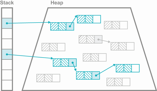
Note that the primitive fields of an object are still allocated at addresses within the heap. As a Java program runs, new objects are created in the heap, and the relationships between the objects changes (as fields are updated). Eventually, the heap will run out of space for new objects to be created. However, many of the objects that have been created will no longer be needed (e.g., temporary objects that were created in one method and not passed to any other method, or returned to the caller).
Space in the heap can therefore be reclaimed, and the program can continue to run. The mechanism by which the platform recovers and reuses heap memory that is no longer in use by application code is called garbage collection.
7.5.2 Mark and sweep
A great example of a simple garbage collection algorithm is mark and sweep, and, in fact, it was the first to be developed (in LISP 1.5, released in 1965).
Note Other automatic memory management techniques exist, such as the reference-counting approach used by languages like Perl, which are arguably simpler (at least superficially), but they aren’t really garbage collection (as per Guy L. Steele “Multiprocessing Compactifying Garbage Collection,” Communications of the ACM 18, no. 9 [September 1975]).
In its simplest form, the mark-and-sweep algorithm pauses all running program threads and starts from the set of objects that are known to be “live”—objects that have a reference in any stack frame (whether that reference is the content of a local variable, method parameter, temporary variable, or some rarer possibility) of any user thread. It then walks through the tree of references from the live objects, marking as live any object found en route. When this has completed, everything left is garbage and can be collected (swept). Note that the swept memory is returned to the JVM, not necessarily to the OS.
What about the nondeterministic pause?
One of the criticisms often leveled at Java (and other environments such as .NET) is that the mark-and-sweep form of garbage collection inevitably leads to Stop-the-World (usually referred to as STW). These are states in which all user threads must be stopped briefly, and this causes pauses that go on for some nondeterministic amount of time.
This issue is frequently overstated. For server software, very few applications have to care about the pause times displayed by the garbage collectors of modern versions of Java. For example, in Java 11 and upward, the default garbage collector is a concurrent collector that does most of its work alongside application threads and minimizes pause time.
Note Developers sometimes dream up elaborate schemes to avoid a pause, or a full collection of memory. In almost all cases, these should be avoided because they usually do more harm than good.
The Java platform provides a number of enhancements to the basic mark-and-sweep approach. One of the simplest is the addition of generational GC. In this approach, the heap isn’t a uniform area of memory—a number of different areas of heap memory participate in the life cycle of a Java object.
Depending on how long an object lives, it can be moved from area to area during collections. References to it can point to several different areas of memory during the lifespan of the object (as illustrated in figure 7.5).

The reason for this arrangement (and the movement of objects) is that analysis of running systems shows that objects tend to either have brief lives or be very long-lived. The different areas of heap memory are designed to allow the platform to exploit this property, by segregating the long-lived objects from the rest.
Please note that figure 7.5 is a simple schematic of a heap designed to illustrate the concept of generational areas. The reality of a real Java heap is a little more complicated and depends upon the collector in use, as we’ll explain later in this chapter.
7.5.3 Areas of memory
The JVM has the following different areas of memory that are used to store objects during their natural life cycle:
-
Eden—Eden is the area of the heap where all objects are initially allocated, and for many objects, this will be the only part of memory in which they ever reside.
-
Survivor—These spaces are where objects that survive a garbage collection cycle (hence the name) are moved. Initially they are moved from Eden, but they may also move between survivor spaces during subsequent GCs.
-
Tenured—The tenured space (aka old generation) is where surviving objects deemed to be “old enough” are moved to (escaping from the survivor spaces). Tenured memory isn’t collected during young collections.
As noted, these areas of memory also participate in collections in different ways. For example, the survivor spaces are really there as a catch-all mechanism, so that short-lived objects created immediately before a collection are handled properly.
If the survivor spaces were not present, then very recently created (but short-lived) objects would be marked as “live” by the GC and would be promoted into Tenured. They would then immediately die but continue to take up space in Tenured until the next time it was collected. This next collection would also happen sooner than necessary due to the improper promotion of what are actually short-lived objects. From a theoretical standpoint, the generational hypothesis also leads us to the idea that there are two types of collections: young and full.
7.5.4 Young collections
A young collection attempts to clear the “young” spaces (Eden and survivor). The process is relatively simple, as described next:
-
All live young objects found during the marking phase are moved.
-
Objects that are sufficiently old (those that have survived enough previous GC runs) go into Tenured.
-
All other young, live objects go into an empty survivor space.
-
At the end, Eden and any recently vacated survivor spaces are ready to be overwritten and reused, because they contain nothing but garbage.
A young collection is triggered when Eden is full. Note that the marking phase must traverse the entire live object graph. If a young object has a reference to a Tenured object, the references held by the Tenured object must still be scanned and marked. Otherwise, the situation could arise where a Tenured object holds a reference to an object in Eden, but nothing else does. If the mark phase doesn’t fully traverse, this Eden object would never been seen and would not be correctly handled. In practice, some performance hacks (e.g. card tables) are used to reduce the potentially high cost of a full marking traversal.
7.5.5 Full collections
When a young collection can’t promote an object to Tenured (due to lack of space), a full collection is triggered. Depending on the collector used, this may involve moving around objects within the old generation. This is done to ensure that the old generation has enough space to allocate a large object if necessary. This is called compacting.
7.5.6 Safepoints
Garbage collection can’t take place without at least a short pause of all application threads. However, threads can’t be stopped at any arbitrary time for GC, because application code can modify the contents of the heap. Instead, certain special times occur where the JVM can be sure that the heap is in a consistent state and GC can take place—these are called safepoints.
One of the simplest examples of a safepoint is “in between bytecode instructions.” The JVM interpreter executes one bytecode at a time, and then loops to take the next bytecode from the stream. Just before looping, that interpreter thread must be finished with any modifications to the heap (e.g., from a putfield), so if the thread stops there, it is “safe.” Once all of the application threads reach a safepoint, then garbage collection can take place.
This is a simple example of a safepoint, but there are others. A more complete discussion of safepoints, and how they impact certain JIT compiler techniques, can be found here: http://mng.bz/Oo8a. Let’s move on from the theoretical discussion and meet some of the garbage collection algorithms in the JVM.
7.5.7 G1: Java’s default collector
G1 is a relatively new collector for the Java platform. It became production-quality at Java 8u40 and was made the default collector with Java 9 (in 2017). It was originally intended as a low-pause collector but in practice has evolved into a general-purpose collector (hence its default status).
It is not only a generational garbage collector, but it is also regionalized, which means that the G1 Java heap divides the heap into equal-sized regions (such as 1, 2, or 4 MB each). Generations still exist, but they are now no longer necessarily contiguous in memory. The new arrangement of equal-sized regions in the heap is illustrated in figure 7.6.

Regionalization has been introduced to support the idea of predictability of GC pauses. Older collectors (such as Parallel) suffered from the problem that once a GC cycle had begun, it needed to run to completion, regardless of how long that took (i.e., they were all-or-nothing).
G1 provides a collection strategy that should not result in longer pause times for larger heaps. It was designed to avoid all-or-nothing behavior, and a key concept for this is the pause goal. This is how long the program can pause for GC before resuming execution. G1 will do everything it can to hit your pause goals, within reason. During a pause, surviving objects are evacuated to another region (like Eden objects being moved to survivor spaces), and the region is placed back on the free list of empty regions.
Young collections in G1 are fully STW and will run to completion. This avoids race conditions between collection and allocation threads (which could occur if young collections ran concurrently with application threads).
Note The generational hypothesis is that only a small fraction of objects encountered during a young collection are still alive. So, the time taken for a young collection should be very small, and much less than the pause goal.
The collection of old objects has a different character from young collections—first, because once objects have reached the old generation, they tend to live for a considerable length of time. Second, the space provided for the old generation tends to be much larger than the young generation.
G1 keeps track of the objects that are moved to the old generation, and when enough old space has been filled (controlled by the InitiatingHeapOccupancyPercent or IHOP, which defaults to 45%), an old collection is started. This is a concurrent collection, because it runs (as far as possible) concurrently with the application threads.
The first piece of this old collection is a concurrent marking phase. This is based on an algorithm that was first described by Dijkstra and Lamport in 1978 (see https://dl.acm.org/doi/10.1145/359642.359655). Once this completes, then a young collection is immediately triggered. This is followed by a mixed collection, which collects old regions based on how much garbage they have in them (which can be deduced from the statistics gathered during the concurrent mark). Surviving objects from the old regions are evacuated into fresh old regions (and compacted).
The nature of the G1 collection strategy also allows the platform to collect statistics on how long (on average) a single region takes to collect. This is how pause goals are implemented—G1 will collect only as many regions as it has time for (although there may be overruns if the last region takes longer to collect than expected).
It is possible that the collection of the entire old generation cannot be completed in a single GC cycle. In this case, G1 just collects a set of regions and then completes the collection, releasing the CPU cores that were being used for GC. Provided that, over a sustained period, the creation of long-lived objects does not outstrip the ability of the GC to reclaim them, all should be well.
In the case that allocation outstrips reclamation for a sustained amount of time, then, as a last-ditch effort, the GC will perform a STW full collection and fully clean and compact the old generation. In practice, this behavior is not seen unless the application is badly struggling.
One other point is worth mentioning: it is possible to allocate objects that are larger than a single region. In practice, this means a large array (often of bytes or other primitives).
Note It would be possible to artificially construct a class that had so many fields that a single object instance was larger than 1 MB, but this would never be done in a practical, real system.
Such objects require a special type of region—a humongous region. These require special treatment by the GC because the space allocated for large arrays must be contiguous in memory. If sufficient free regions are adjacent to each other, they can be converted to a single humongous region and the array can be allocated.
If there isn’t anywhere in memory where the array can be allocated (even after a young collection), then memory is said to be fragmented. The GC must perform a fully STW and compacting collection to try to free up sufficient space for the allocation.
G1 is established as a very effective collector across a wide variety of workloads and application types. However, for some workloads (e.g., those that need pure throughput or are still running on Java 8), then another collector, such as Parallel, may be of use.
7.5.8 The Parallel collector
The Parallel collector was the default until Java 8, and it can still be used as an alternative choice to G1 today. The name Parallel needs a bit of explanation, because concurrent and parallel are both used to describe properties of GC algorithms. They sound as though they should mean the same thing, but in fact they have two totally different meanings, as described here:
-
Concurrent—GC threads can run at the same time as application threads.
-
Parallel—The GC algorithm is multithreaded and can use multiple cores.
The terms are in no way equivalent. Instead, it’s better to think of them as the opposites to two other GC terms—concurrent is the opposite of STW, and parallel is the opposite of single-threaded.
In some collectors (including Parallel), the heap is not regionalized. Instead, the generations are contiguous areas of memory, which have headroom to grow and shrink as needed. In this heap configuration there are two survivor spaces. They are sometimes referred to as From and To, and one of the survivor spaces is always empty unless a collection is under way.
Note Very old versions of Java also had a space called PermGen (or Permanent Generation). This is where memory was allocated for the JVM’s internal structures, such as the definitions of classes and methods. PermGen was removed in Java 8, so if you find any resources that refer to it, then they are old and likely to be outdated.
Parallel is a very efficient collector—the most efficient one available in mainstream Java—but it comes with a drawback: it has no real pause goal capability and old collections (that are STW) must run to completion, regardless of how long it takes.
Some developers sometimes ask questions about the complexity (aka “big-O”) behavior of GC algorithms. However, this is not really a useful question to ask. GC algorithms are very general, and they are required to behave acceptably across an entire range of possible workloads. Focusing only on their asymptotic behavior is not all that useful, and it is definitely not a suitable proxy for their general-case performance.
Garbage collection is always about trade-offs, and the trade-offs that G1 makes are very good for most workloads (so much so that many developers can just ignore them). However, the trade-offs always exist, whether or not the developer is aware of them. Some applications cannot ignore the trade-offs and must choose to care about the details of the GC subsystem, either by changing collection algorithm or by tuning using GC parameters.
7.5.9 GC configuration parameters
The JVM ships with a huge number of useful parameters (at least a hundred) that can be used to customize many aspects of the runtime behavior of the JVM. In this section, we’ll discuss some of the basic switches that pertain to garbage collection.
If a switch starts with -X:, it’s nonstandard and may not be portable across JVM implementations (such as HotSpot or Eclipse OpenJ9). If it starts with -XX:, it’s an extended switch and isn’t recommended for casual use. Many performance-relevant switches are extended switches.
Some switches are Boolean in effect and take a + or - in front of them to turn it on or off. Other switches take a parameter, such as -XX:CompileThreshold=20000 (which would set the number of times a method needs to be called before being considered for JIT compilation to 20000). Table 7.1 lists the basic GC switches and displays the default value (if any) of the switch.
Table 7.1 Basic garbage collection switches
One unfortunately common technique is to set the size of -Xms to the same as -Xmx. This then means that the process will run with exactly that heap size and will not resize during execution. Superficially, this makes sense, and it gives the illusion of control to the developer. However, in practice, this approach is an antipattern. Modern GCs have good dynamic sizing algorithms, and artificially constraining them almost always does more harm than good.
Note In 2022, best practice for most workloads, in the absence of any other evidence, is to set Xmx and not to set Xms at all.
It’s also worth noting the behavior of the JVM in a container. For Java 11 and 17, “physical memory” means the container limit, so the heap max size must fit within any container limit and with space for the non-Java heap memory and any other processes other than the JVM. Early versions of Java 8 do not necessarily respect container limits, so the advice is always to upgrade to Java 11 if you are running your application in containers. For the G1 collector, two other settings may be useful during tuning exercises—they’re shown in table 7.2.
Table 7.2 Flags for the G1 collector
|
Indicates to G1 that it should try to pause for no more than 50 ms during one collection | |
|
Indicates to G1 that it should try to run for at least 200 ms between collections |
The switches can be combined, such as to set a maximum pause goal of 50 ms with pauses occurring no closer together than 200 ms. Of course, there’s a limit on how hard the GC system can be pushed. There has to be enough pause time to take out the trash. A pause goal of 1 ms per 100 years is certainly not going to be attainable or honored.
In the next section, we’ll take a look at JIT compilation. For many programs, this is a major contributing factor to producing performant code. We’ll look at some of the basics of JIT compilation, and at the end of the section, we’ll explain how to switch on logging of JIT compilation to enable you to tell which of your methods are being compiled.
7.6 JIT compilation with HotSpot
As we discussed in chapter 1, the Java platform is perhaps best thought of as “dynamically compiled.” Some application and framework classes undergo further compilation at runtime to transform them into machine code that can be directly executed.
This process is called just-in-time (JIT) compilation, or just JITing, and it usually occurs on one method at a time. Understanding this process is often key to identifying the important parts of any sizable codebase.
Let’s look at some good basic facts about JIT compilation:
-
Virtually all modern JVMs will have a JIT compiler of some sort.
-
Compiled methods run much, much faster than interpreted code.
-
It makes sense to compile the most heavily used methods first.
-
When doing JIT compilation, it’s always important to take the low-hanging fruit first.
This last point means that we should look at the compiled code first, because under normal circumstances, any method that is still in an interpreted state hasn’t been run as often as one that has been compiled. (Occasionally a method will fail compilation, but this is quite rare.)
Methods start off being interpreted from their bytecode representation, with the JVM keeping track of how many times a method has been called (and some other statistics). When a threshold value is reached, if the method is eligible, a JVM thread will compile the bytecode to machine code in the background. If compilation succeeds, all further calls to the method will use the compiled form, unless something happens to invalidate it or otherwise cause deoptimization.
Depending on the exact nature of the code in a method, a compiled method can be vastly faster than the same method in interpreted mode. The figure of “up to 100 times faster” is sometimes given, but this is an extremely rough rule of thumb. The nature of JIT compilation changes the executed code so much that any kind of single number is misleading. Understanding which methods are important in a program, and which important methods are being compiled, is quite often a major technique in improving performance.
7.6.1 Why have dynamic compilation?
A question that is sometimes asked is, why does the Java platform bother with dynamic compilation? Why isn’t all compilation done up front (like C++)? The first answer is usually that having platform-independent artifacts (.jar and .class files) as the basic unit of deployment is much less of a headache than trying to deal with a different compiled binary for each platform being targeted.
An alternative, and more ambitious, answer is that languages that use dynamic compilation have more information available to their compiler. Specifically, ahead-of-time (AOT) compiled languages don’t have access to any runtime information, such as the availability of certain instructions or other hardware details, or any statistics on how the code is running. This opens the intriguing possibility that a dynamically compiled language like Java could actually run faster than AOT-compiled languages.
Note Direct, AOT compilation of Java bytecode to machine code (aka “static Java”) is a live area of research in the Java community but, unfortunately, is outside the scope of this book.
For the rest of this discussion of the mechanics of JITing, we’ll be speaking specifically about the JVM called HotSpot. A lot of the general discussion will apply to other VMs, but the specifics could vary a lot.
We’ll start by introducing the different JIT compilers that ship with HotSpot and then explain two of the most powerful optimizations available from HotSpot—inlining and monomorphic dispatch. We’ll conclude this section by showing how to turn on logging of method compilation, so that you can see exactly which methods are being compiled. Let’s get started by introducing HotSpot.
7.6.2 Introduction to HotSpot
HotSpot is the JVM that Oracle acquired when it bought Sun Microsystems (it already owned a JVM called JRockit, which was originally developed by BEA Systems). HotSpot is the JVM that forms the basis of OpenJDK. It’s capable of running in two separate modes: client and server.
In the old days, the mode could be chosen by specifying the -client or -server switch to the JVM on startup. Each of these modes has different applications that they can be preferred for.
The C1 compiler was originally intended for use in GUI applications. This is an area where consistency of operation is prized, so C1 (sometimes called the client compiler) tends to make more conservative decisions when compiling. It can’t pause unexpectedly while it backs out an optimization decision that turned out to be incorrect or based on a faulty assumption. It has a fairly low compilation threshold—a method must be executed 1500 times before being eligible for compilation—so it has a relative short warmup period.
By contrast, the server compiler (C2) makes aggressive assumptions when compiling. To ensure that the code that’s run is always correct, C2 adds a quick runtime check (usually called a guard condition) that the assumption it made is valid. If not, it backs out the aggressive compilation and often tries something else. This aggressive approach can yield far better performance than the rather risk-averse client compiler.
C2 has a much higher inlining threshold than C1. By default, a method is not eligible for C2 compilation until it hits 10,000 invocations, which implies a much longer warmup time.
Historically, a form of Java was developed called real-time Java, and some developers wonder why code that has a need for high performance doesn’t simply use this platform (which is a separate JVM, not a HotSpot option). The answer is that a real-time system is not, despite common myth, necessarily the fastest system.
Real-time programming is really about the guarantees that can be made. In statistical terms, a real-time system seeks to reduce the variance of the time taken to perform certain operations and is prepared to sacrifice a certain amount of mean latency to do so. Overall performance may be slightly sacrificed to attain more consistent running. Teams in search of higher performance are usually in search of lower mean latency, even at the cost of higher variance, so the aggressive optimizations of the server compiler are especially suitable.
In modern JVMs, the client and server compilers are both used—the client compiler is used early on, and the advanced server-class optimizations are used after the application has warmed up. This dual use is known as tiered compilation. Our next topic is one that is extensively used by all of the JIT compilers.
7.6.3 Inlining methods
Inlining is one of the most powerful techniques that HotSpot has at its disposal. It works by eliminating the call to the inlined method and instead places the code of the called method inside the caller.
One of the advantages of the platform is that the compiler can make the decision to inline based on decent runtime statistics about how often the method is called and other factors (e.g., will it make the caller method too large and potentially affect code caches). HotSpot’s compiler can make much smarter decisions about inlining than ahead-of-time compilers.
Some developers incorrectly assume that an accessor method (a public getter accessing a private member variable) can’t be inlined by HotSpot. Their reasoning is that because the variable is private, the method call can’t be optimized away, because access to it is prohibited outside the class. This is incorrect.
HotSpot can and will ignore access control when compiling methods to machine code and will replace an accessor method with a direct access to the private field. This doesn’t compromise Java’s security model, because all of the access control was checked when the class was loaded or linked.
Inlining of methods is entirely automatic, and under almost all circumstances, the default parameter values are fine. Switches are available to control what size of methods will be inlined and how often a method needs to be called before becoming a candidate.
These switches are mostly useful for the curious programmer to get a better understanding of how the inlining part of the internals works. They aren’t often useful for production code and should be considered something of a last resort as a performance technique, because they may well have other unpredictable effects on the performance of the runtime system.
7.6.4 Dynamic compilation and monomorphic calls
One example of this type of aggressive optimization is that of the monomorphic call. This is an optimization that’s based on the observation that, in most circumstances, a method call on an object, like this:
will only ever be called by one type of object. Another way of saying this is that the call site obj.callMyMethod() will almost never encounter both a class and its subclass. In this case, the Java method lookup can be replaced with a direct call to the compiled code corresponding to callMyMethod().
Note Monomorphic dispatch provides an example of the JVM runtime profiling, allowing the platform to perform optimizations that an AOT language like C++ simply can’t.
There’s no technical reason why the getInstance() method can’t return an object of type MyActualClassNotInterface under some circumstances and an object of some subclass under others. To guard against the possibility that this happens, getInstance() will not be put forward for monomorphic optimization unless the exact same type has been seen at the call site every single time, until the compilation threshold is reached. A runtime test to check the type of obj is also inserted into the compiled code for future calls. If this expectation is ever violated, the runtime backs out the optimization without the program ever noticing or ever doing anything incorrect.
This is a fairly aggressive optimization that is only ever performed by the server compiler. The client compiler does not do this.
7.6.5 Reading the compilation logs
Let’s take a look at an example to illustrate how you can use the log messages output by the JIT compiler. The Hipparcos star catalog lists details about stars that can be observed from Earth. Our example application processes the catalog to generate star maps of the stars that can be seen on a given night, in a given location.
Let’s look at some example output that shows which methods are being compiled when we run our star map application. The key JVM flag we’re using is -XX:+Print-Compilation. This is one of the extended switches we briefly discussed earlier. Adding this switch to the command line used to start the JVM tells the JIT compilation threads to add messages to the standard log. These messages indicate when methods have passed the compilation threshold and been turned into machine code as follows:
1 java.lang.String::hashCode (64 bytes)
2 java.math.BigInteger::mulAdd (81 bytes)
3 java.math.BigInteger::multiplyToLen (219 bytes)
4 java.math.BigInteger::addOne (77 bytes)
5 java.math.BigInteger::squareToLen (172 bytes)
6 java.math.BigInteger::primitiveLeftShift (79 bytes)
7 java.math.BigInteger::montReduce (99 bytes)
8 sun.security.provider.SHA::implCompress (491 bytes)
9 java.lang.String::charAt (33 bytes)
1% ! sun.nio.cs.SingleByteDecoder::decodeArrayLoop @ 129 (308 bytes)
...
39 sun.misc.FloatingDecimal::doubleValue (1289 bytes)
40 org.camelot.hipparcos.DelimitedLine::getNextString (5 bytes)
41 ! org.camelot.hipparcos.Star::parseStar (301 bytes)
...
2% ! org.camelot.CamelotStarter::populateStarStore @ 25 (106 bytes)
65 s java.lang.StringBuffer::append (8 bytes)
This is pretty typical output from PrintCompilation. These lines indicate which methods have been deemed sufficiently “hot” to be compiled. As you might expect, the first methods to be compiled will likely be platform methods (such as String ::hashCode()). Over time, application methods (such as the org.camelot.hipparcos .Star::parseStar() method, which is used in the example to parse a record from the astronomical catalog) will also be compiled.
The output lines have a number, which indicates in which order the methods are compiled on this run. Note that this order may change slightly between runs due to the dynamic nature of the platform. Some of the other fields follow:
OSR means that the method was compiled and replaced the interpreted version in running code. Note that OSR methods have their own numbering scheme, starting at 1.
When looking at sample output logs on code that is run using the server compiler (C2), you’ll occasionally see lines like “made not entrant” and “made zombie.” These lines mean that a particular method, which had been compiled, has now been invalidated, usually because of a class loading operation.
7.6.6 Deoptimization
HotSpot is capable of deoptimizing code that’s based on an assumption that turned out not to be true. In many cases, it then reconsiders and tries an alternative optimization. Thus, the same method may be deoptimized and recompiled several times.
Over time, you’ll see that the number of compiled methods stabilizes. Code reaches a steady, compiled state and largely remains there. The exact details of which methods get compiled can depend on the exact JVM version and OS platform in use. It’s a mistake to assume that all platforms will produce the same set of compiled methods and that the compiled code for a given method will be roughly the same size across platforms. As with so much else in the performance space, this should be measured, and the results may surprise. Even a fairly innocent-looking Java method has proved to have a factor-of-five difference between Mac and Linux in terms of the machine code generated by JIT compilation.
Measurement is always necessary. Fortunately, modern JVMs ship some great tools to facilitate deep-dive performance analysis. Let’s take a look at them.
7.7 JDK Flight Recorder
Historically, the Flight Recorder and Mission Control tools (usually referred to as JFR and JMC) were obtained by Oracle as part of the acquisition of BEA Systems back in 2008. The two components work together—JFR is a low-overhead, event-based profiling engine with a high-performance backend for writing events in a binary format, whereas JMC is a GUI tool for examining a data file created by JFR from the telemetry of a single JVM.
The tools were originally part of the tooling offering for BEA’s JRockit JVM and were moved to the commercial version of Oracle JDK as part of the process of merging JRockit with HotSpot. After the release of JDK 9, Oracle changed the release model of Java and announced that JFR and JMC would become open source tools. JFR was contributed to OpenJDK and was delivered in JDK 11 as JEP 328. JMC was spun out into a standalone open-source project and exists today as a separate download.
Note Java 14 introduced a new feature to JFR: the ability for JFR to produce a continuous stream of events. This change provides a callback API to enable events to be handled immediately, rather than by parsing a file after the fact.
One issue, however, is that because JFR and JMC only recently became open source tools, many Java developers are not aware of their considerable capabilities. Let’s take this opportunity to introduce JMC and JFR from the beginning.
7.7.1 Flight Recorder
JFR first became available as open source as part of OpenJDK 11, so to make use of it, you need to be running that version (or a more recent one). The technology was also back-ported to OpenJDK 8 and is available for versions 8u262 and upward.
There are various ways to create a JFR recording, but we’re going to look at two in particular: the use of command-line arguments when starting up a JVM and the use of jcmd.
First, let’s see what command-line switches we need to start JFR up at process start time. The key switch follows:
This can either be done as a one-off dump file or a continuous ring buffer, and a large number of individual command-line options control what data is being captured.
In addition, JFR can capture more than a hundred different possible metrics. Most of these are very low-impact, but some do incur some overhead. Managing the configuration of all of these metrics individually would be a huge task.
Instead, to simplify the process, JFR uses profiling configuration files. These are simple XML files that contain configurations for each metric and whether or not it should be captured. The standard JDK download contains two basic files: default.jfc and profile.jfc.
The default level of recording is designed to be extremely low overhead and to be useable by basically every production Java process. The profile.jfc configuration contains more detailed information, but this, of course, comes at a higher runtime cost.
Note As well as the two supplied files, it is possible to create a custom configuration file that contains just the data points that are wanted. The JMC tool has a template manager that enables easy creation of these files.
As well as the settings file, other options that can be passed include the filename in which to store the recorded data and how much data to keep (in terms of the age of the data points). For example, an overall JFR command line might look like this (given on a single line):
Note When JFR was a part of the commercial build, it was unlocked with the -XX:+UnlockCommercialFeatures switch. However, Oracle JDK 11+ emits a warning when the -XX:+UnlockCommercialFeatures option is used. This is because all the commercial features have been open sourced, and because the flag was never part of OpenJDK, it does not make sense to continue to use it. In OpenJDK builds, using the commercial features flag results in an error.
One of the great features of JFR is that it does not need to be configured at the process start. Instead, it can be controlled from the command line using the jcmd command, as shown here:
$ jcmd <pid> JFR.start name=Recording1 settings=default
$ jcmd <pid> JFR.dump filename=recording.jfr
$ jcmd <pid> JFR.stop
JFR also provides a JMX API for controlling JFR recordings as well. However, no matter how JFR is activated, the end result is the same—a single file per profiling run per JVM. The file contains a lot of binary data and is not human-readable, so we need some sort of tool to extract and visualize the data.
7.7.2 Mission Control
JDK Mission Control (JMC) is a graphical tool used to display the data contained in JFR output files. It is started up from the jmc command. This program used to be bundled with the Oracle JDK download but is now available separately from https://jdk.java.net/jmc/.
The startup screen for Mission Control can be seen in figure 7.7. After loading the file, JMC performs some automated analysis on it to identify any obvious problems present in the recorded run.

Note To profile, Flight Recorder must, of course, be enabled on the target application. As well as using a previously created file, it is also possible to dynamically attach it after the application has already started. For the latter option, JMC provides a tab on the left of the top-left panel labeled JVM Browser for attaching it dynamically to local applications.
One of the first screens encountered in JMC is the overview telemetry screen that shows a high-level dashboard of the overall health of the JVM. This can be seen in figure 7.8

The major subsystems of the JVM all have dedicated screens to enable deep-dive analysis. For example, garbage collection has an overview screen to show the GC events over the lifetime of the JFR file. The “Longest Pause” display at the bottom allows the user to see where any anomalously long GC events have occurred over the timeline, as shown in figure 7.9

In the detailed profile configuration, it is also possible to see the individual events where new allocation buffers (TLABs) are handed out to application threads. We can see a much more accurate view of allocation within the process. The view looks like that shown in figure 7.10. This view allows developers to easily see which threads are allocating the most memory—in this example, it’s a thread that is consuming data from Apache Kafka topics.

The other major subsystem of the JVM is the JIT compiler, and JMC allows us to dig into the details of how the compiler is working, as we can see in figure 7.11.

A key resource is the available memory in the JIT compiler’s code cache. This is the area of memory where the compiled version of methods are stored. The usage of the code cache can be visualized in JMC— an example is shown in figure 7.12.
For processes that have a lot of compiled methods, this area of memory can be exhausted, causing the process to not reach peak performance.
JMC also includes a method-level profiler, which works in a very similar way to the one found in VisualVM or commercial tools such as JProfiler or YourKit. Figure 7.13 shows a typical result.

One of the more advanced screens within JMC is the VM Operations view, which shows some of the internal operations the JVM performs and how long they take. This is not a view that we would expect to need for every analysis, but it would be potentially useful for detecting certain types of less-common problem. We can see a typical usage in figure 7.14.

JMC can be used to diagnose a single JVM, and this is a great capability to have. However, this use case does not scale to examining an entire cluster (or full application). In addition, modern systems frequently need a monitoring, or observability, solution as well as the deep-dive capability.
The classic JFR model of a recording file (and one-file JVM) does not make this easy. It is not a good fit for the stream of telemetry data delivered over the network to a SaaS provider or internal tool. Some vendors (e.g., New Relic and DataDog) do provide a JFR capability, but the use of these techniques is still somewhat niche.
Fortunately, the JFR Streaming API that was introduced with Java 14 provides an excellent building block for the observability use case as well as a deep dive. The community as a whole has tended not to adopt the non-LTS releases of Java, however. This means that it is likely that only with the arrival of Java 17 (which is LTS) will we see widespread adoption of a Java version that supports the streaming form of JFR.
Performance tuning isn’t about staring at your code and praying for enlightenment or applying canned quick fixes. Instead, it’s about meticulous measurement, attention to detail, and patience. It’s about persistent reduction of sources of error in your tests, so that the true sources of performance problems emerge.
In this chapter, we’ve been able to give only a brief introduction to a rich and varied topic. There is so much more to explore, and the interested reader should consult a dedicated text, such as Optimizing Java by Ben Evans, James Gough, and Chris Newland (O’Reilly Media, May 2018).
Summary
-
The JVM is an incredibly powerful and sophisticated runtime environment.
-
The JVM’s nature can make it sometimes challenging to optimize the code within.
-
You have to measure to get an accurate idea of where the problems really are.
-
Pay particular attention to the garbage collection subsystem and the JIT compiler.
-
Learn to read the logs and other indicators of the platform—tools aren’t always available.