- Understanding the basics of the transformer neural network architecture
- Using the Generative Pretrained Transformer (GPT) to generate text
In this chapter and the following chapter, we cover some representative deep transfer learning modeling architectures for NLP that rely on a recently popularized neural architecture—the transformer 1—for key functions. This is arguably the most important architecture for natural language processing (NLP) today. Specifically, we will be looking at modeling frameworks such as GPT,2 Bidirectional Encoder Representations from Transformers (BERT),3 and multilingual BERT (mBERT).4 These methods employ neural networks with even more parameters than the deep convolutional and recurrent neural network models that we looked at in the previous two chapters. Despite the larger size, these frameworks have exploded in popularity because they scale comparatively more effectively on parallel computing architecture. This enables even larger and more sophisticated models to be developed in practice. To make the content more digestible, we have split the coverage of these models into two chapters/parts: we cover the transformer and GPT neural network architectures in this chapter, whereas in the next chapter, we focus on BERT and mBERT.
Until the arrival of the transformer, the dominant NLP models relied on recurrent and convolutional components, as we saw in the previous two chapters. Additionally, the best sequence modeling and transduction problems, such as machine translation, relied on an encoder-decoder architecture with an attention mechanism to detect which parts of the input influence each part of the output. The transformer aims to replace the recurrent and convolutional components entirely with attention.
The goal of this and the following chapters is to provide you with a working understanding of this important class of models and to help you develop a good sense about where some of its beneficial properties come from. We introduce an important library—aptly named transformers—that makes the analysis, training, and application of these types of models in NLP particularly user-friendly. Additionally, we use the tensor2tensor TensorFlow package to help visualize attention functionality. The presentation of each transformer-based model architecture—GPT, BERT, and mBERT—is followed by representative code applying it to a relevant task.
GPT, which was developed by OpenAI,5 is a transformer-based model that is trained with a causal modeling objective : to predict the next word in a sequence. It is also particularly suited for text generation. We show how to employ pretrained GPT weights for this purpose with the transformers library.
BERT is a transformer-based model that we encountered briefly in chapter 3. It was trained with the masked modeling objective : to fill in the blanks. Additionally, it was trained with the next sentence prediction task: to determine whether a given sentence is a plausible subsequent sentence after a target sentence. Although not suited for text generation, this model performs well on other general language tasks such as classification and question answering. We have already explored classification in some detail, so we will use the question-answering task to explore this model architecture in more detail than we did in chapter 3.
mBERT, which stands for Multilingual BERT, is effectively BERT pretrained on over 100 languages simultaneously. Naturally, this model is particularly well-suited for cross-lingual transfer learning. We will show how the multilingual pretrained checkpoint can facilitate creating BERT embeddings for languages that were not even originally included in the multilingual training corpus. Both BERT and mBERT were created at Google.
We begin the chapter with a review of fundamental architectural components and visualize them in some detail with the tensor2tensor package. We follow that up with a section overviewing the GPT architecture, with text generation as a representative application of pretrained weights. The first section of chapter 8 then covers BERT, which we apply to the very important question-answering application as a representative example in a stand-alone section. Chapter 8 concludes with an experiment showing the transfer of pretrained knowledge from mBERT pretrained weights to a BERT embedding for a new language. This new language was not initially included in the multilingual corpus used to generate the pretrained mBERT weights. We use the Ghanaian language Twi as the illustrative language in this case. This example also provides an opportunity to further explore fine-tuning pretrained BERT weights on a new corpus. Note that Twi is an example of a low-resource language—one for which high-quality training data is scarce, if available at all.
7.1 The transformer
In this section, we look closer at the fundamental transformer architecture behind the neural model family covered by this chapter. This architecture was developed at Google6 and was motivated by the observation that the best-performing translation models up to that point employed convolutional and recurrent components in conjunction with a mechanism called attention.
More specifically, such models employ an encoder-decoder architecture, where the encoder converts the input text into some intermediate numerical vector representation, typically called the context vector, and a decoder that converts this vector into output text. Attention allows for better performance in these models by modeling dependencies between parts of the output and the input. Typically, attention had been coupled with recurrent components. Because such components are inherently sequential—the internal hidden state at any given position t depends on the hidden state at the previous position t-1—parallelization of the processing of a long input sequence is not an option. Parallelization across such input sequences, on the other hand, quickly runs into GPU memory limitations.
The transformer discards recurrence and replaces all functionality with attention. More specifically, it uses a flavor of attention called self-attention. Self-attention is essentially attention as previously described but applied to the same sequence as both input and output. This allows it to learn the dependencies between every part of the sequence and every other part of the same sequence. Figure 7.3 will revisit and illustrate this idea in more detail, so don’t worry if you can’t visualize it fully yet. These models have better parallelizability versus the aforementioned recurrent models. Looking ahead, we address exactly the reason for this in section 7.1.2, where we use the example sentence, “He didn’t want to talk about cells on the cell phone because he considered it boring,” to study how various aspects of the infrastructure work.
Now that we understand the basics of the motivation behind this architecture, let’s take a look at a simplified bird’s-eye-view representation of the various building blocks, shown in figure 7.1.
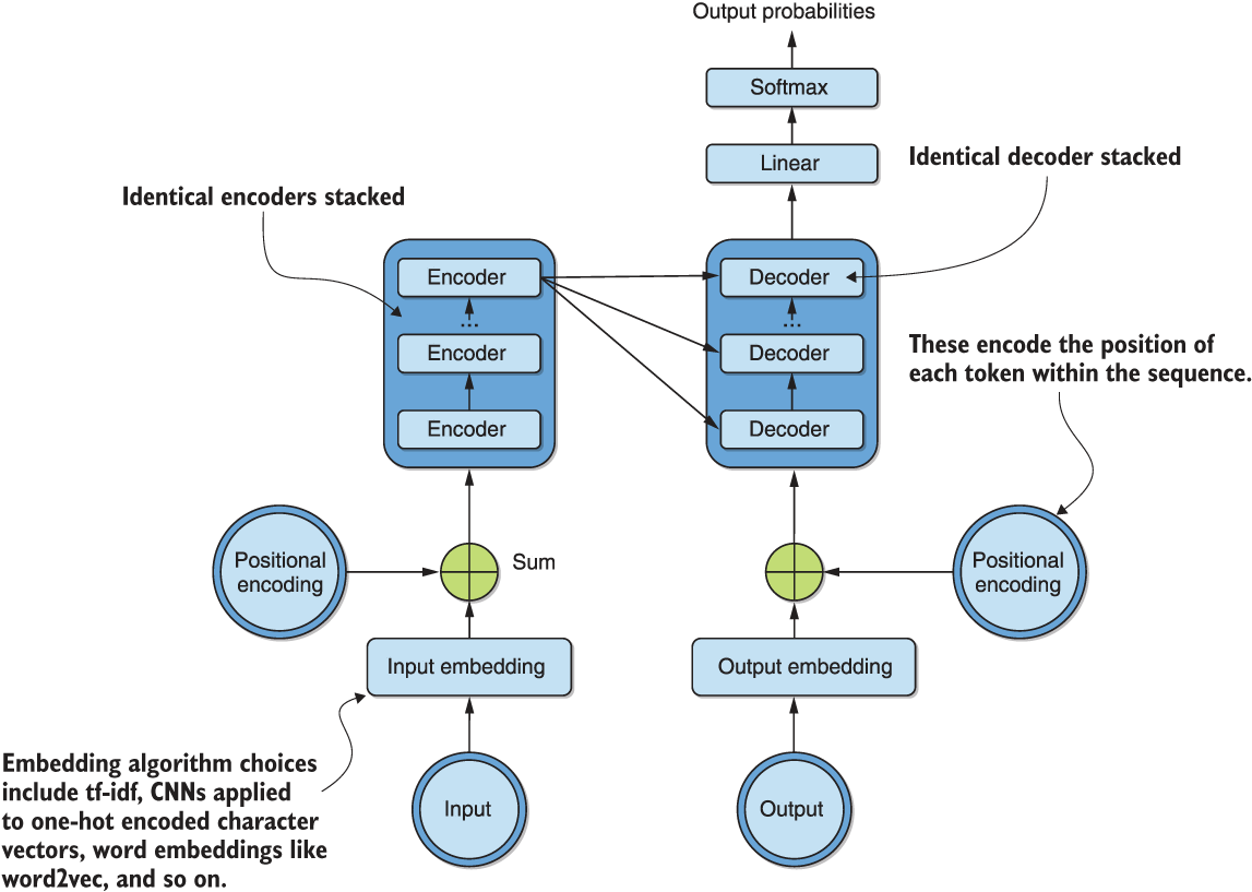
Figure 7.1 A high-level representation of the transformer architecture, showing stacked encoders, decoders, input/output embeddings, and positional encodings
We see from the figure that identical encoders are stacked on the encoding, or left, side of the architecture. The number of stacked encoders is a tunable hyperparameter, with the original paper working with six. Similarly, on the decoding, or right, side of the architecture, six identical decoders are stacked. We also see that both the input and output are converted into vectors using an embedding algorithm of choice. This could be a word embedding algorithm such as word2vec, or even a CNN applied to one-hot encoded character vectors very similar to those we encountered in the previous chapter. Additionally, we encode the sequential nature of the inputs and outputs using positional encodings. These allow us to discard recurrent components while maintaining sequential awareness.
Each encoder can be roughly decomposed into a self-attention layer followed by a feedforward neural network, as illustrated in figure 7.2.
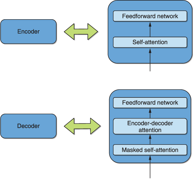
Figure 7.2 A simplified decomposition of the encoder and decoder into self-attention, encoder-decoder attention, and feedforward neural networks
As can be seen in the figure, each decoder can be similarly decomposed with the addition of an encoder-decoder attention layer between the self-attention layer and the feedforward neural network. Note that in the self-attention of the decoder, future tokens are “masked” when computing attention for that token—we will return to this at a more appropriate time. Whereas the self-attention learns the dependencies of every part of its input sequence and every other part of the same sequence, encoder-decoder attention learns similar dependencies between the inputs to the encoder and decoder. This process is similar to the way attention was initially used in the sequence-to-sequence recurrent translation models.
The self-attention layer in figure 7.2 can further be refined into multihead attention—a multidimensional analog of self-attention that leads to improved performance. We analyze self-attention in further detail in the following subsections and build on the insights gained to cover multihead attention. The bertviz package7 is used for visualization purposes to provide further insights. We later close the chapter by loading a representative transformer translation model with the transformers library and using it to quickly translate a couple of English sentences into the low-resource Ghanaian language, Twi.
7.1.1 An introduction to the transformers library and attention visualization
Before we discuss in detail how various components of multihead attention works, let’s visualize it for the example sentence, “He didn’t want to talk about cells on the cell phone because he considered it boring.” This exercise also allows us to introduce the transformers Python library from Hugging Face. The first step to doing this is to obtain the required dependencies using the following commands:
!pip install tensor2tensor
!git clone https:/ /github.com/jessevig/bertviz.git
Note Recall from the previous chapters that the exclamation sign (!) is required only when executing in a Jupyter environment, such as the Kaggle environment we recommend for these exercises. When executing via a terminal, it should be dropped.
The tensor2tensor package contains the original authors’ implementation of the transformers architecture, together with some visualization utilities. The bertviz library is an extension of these visualization utilities to a large set of the models within the transformers library. Note that it requires JavaScript to be activated to render its visualization (we show you how to do that in the companion Kaggle notebook).
The transformers library can be installed with the following:
!pip install transformers
Note that it is already installed on new notebooks on Kaggle.
For our visualization purposes, we look at the self-attention of a BERT encoder. It is arguably the most popular flavor of the transformers-based architecture and similar to the encoder in the encoder-decoder architecture of the original architecture in figure 7.1. We will visualize BERT architecture explicitly in figure 8.1 of section 8.1. For now, all you need to note is that the BERT encoder is identical to that of the transformer.
For any pretrained model that you want to load in the transformers library, you need to load a tokenizer as well as the model using the following commands:
from transformers import BertTokenizer, BertModel                                         ❶
model = BertModel.from_pretrained('bert-base-uncased', output_attentions=True)            ❷
tokenizer = BertTokenizer.from_pretrained('bert-base-uncased', do_lower_case=True)        ❸
❶ The transformers BERT tokenizer and model
❷ Loads the uncased BERT model, making sure to output attention
❸ Loads the uncased BERT tokenizer
Note that the uncased BERT checkpoint we are using here is the same as what we used in chapter 3 (listing 3.7) when we first encountered the BERT model through TensorFlow Hub.
You can tokenize our running example sentence, encode each token as its index in the vocabulary, and display the outcome using the following code:
sentence = "He didnt want to talk about cells on the cell phone because he considered it boring"
inputs = tokenizer.encode(sentence, return_tensors='tf', add_special_tokens=True)                            ❶
print(inputs)
❶ Changing return_tensors to "pt" will return PyTorch tensors.
This yields the following output:
tf.Tensor(
[[  101  2002  2134  2102  2215  2000  2831  2055  4442  2006  1996  3526
   3042  2138  2002  2641  2009 11771   102]], shape=(1, 19), dtype=int32)
We could have easily returned a PyTorch tensor simply by setting return_tensors='pt'. To see which tokens these indices correspond to, we can execute the following code on the inputs variable:
tokens = tokenizer.convert_ids_to_tokens(list(inputs[0]))     ❶
print(tokens)
❶ Extracts a sample of batch index 0 from the inputs list of lists
This produces the following output:
['[CLS]', 'he', 'didn', '##t', 'want', 'to', 'talk', 'about', 'cells', 'on', 'the', 'cell', 'phone', 'because', 'he', 'considered', 'it', 'boring', '[SEP]']
We notice immediately that the “special tokens” we requested via the add_special _tokens argument when encoding the inputs variable refers to the '[CLS]' and '[SEP]' tokens in this case. The former indicates the beginning of a sentence/ sequence, whereas the latter indicates the separation point between multiple sequences or the end of a sequence (as in this case). Note that these are BERT-dependent, and you should check the documentation of each new architecture you try to see which special tokens it uses. The other thing we notice from this tokenization exercise is that the tokenization is subword—notice how didnt was split into didn and ##t, even without the apostrophe (’), which we deliberately omitted.
Let’s proceed to visualizing the self-attention layer of the BERT model we have loaded by defining the following function:
from bertviz.bertviz import head_view                           ❶

def show_head_view(model, tokenizer, sentence):                 ❷
    input_ids = tokenizer.encode(sentence, return_tensors='pt', add_special_tokens=True)                                   ❸
    attention = model(input_ids)[-1]                            ❹
    tokens = tokenizer.convert_ids_to_tokens(list(input_ids[0]))
    head_view(attention, tokens)                                ❺

show_head_view(model, tokenizer, sentence)                      ❻
❶ The bertviz attention head visualization method
❷ Function for displaying the multiheaded attention
❸ Be sure to use PyTorch with bertviz.
❺ Calls the internal bertviz method to display self-attention
❻ Calls our function to render visualization
Figure 7.3 shows the resulting self-attention visualization of the final BERT layer of our example sentence. You should play with the visualization and scroll through the visualizations of the various words for the various layers. Note that not all the attention visualizations may be as easy to interpret as this example, and it may take some practice to build intuition for it.
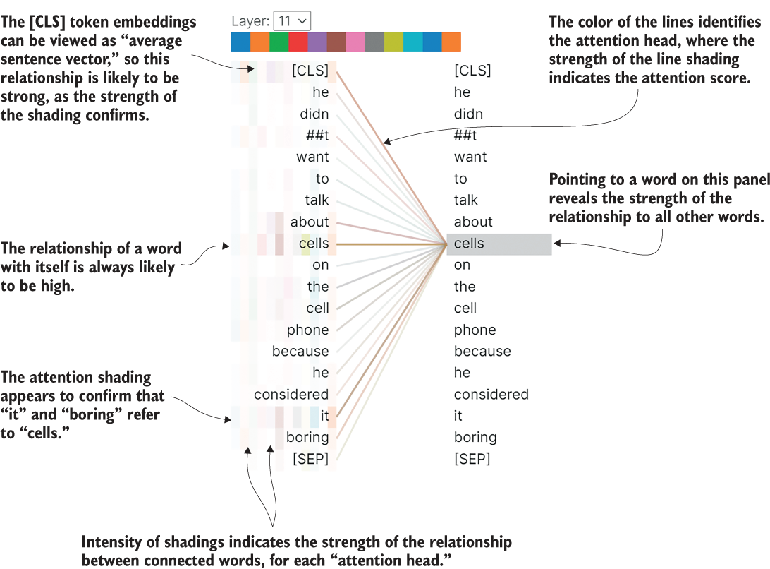
Figure 7.3 Self-attention visualization in the final encoding layer of the pretrained uncased BERT model for our example sentence. It reveals that “cells” is associated with “it” and “boring.” Note that this is a multihead view, with the shadings in each single column representing each head. Multiheaded attention is addressed in detail in section 7.1.2.
That was it! Now that we have a sense for what self-attention does, having visualized it in figure 7.3, let’s get into the mathematical details of how it works. We first start with self-attention in the next subsection and then extend our knowledge to the full multiheaded context afterward.
7.1.2 Self-attention
Consider again the example sentence, “He didn’t want to talk about cells on the cell phone because he considered it boring.” Suppose we wanted to figure out which noun the adjective “boring” was describing. Being able to answer a question like this is an important ability a machine needs to have to understand context. We know it refers to “it,” which refers to “cells,” naturally. This was confirmed by our visualization in figure 7.3. A machine needs to be taught this sense of context. Self-attention is the method that accomplishes this in the transformer. As every token in the input is processed, self-attention looks at all other tokens to detect possible dependencies. Recall that we achieved this same function with bidirectional LSTMs in the previous chapter.
So how does self-attention actually work to accomplish this? We visualize the essential ideas of this in figure 7.4. In the figure, we are computing the self-attention weight for the word “boring.” Before delving into further detail, please note that once the various query, key, and value vectors for the various words are obtained, they can be processed independently.
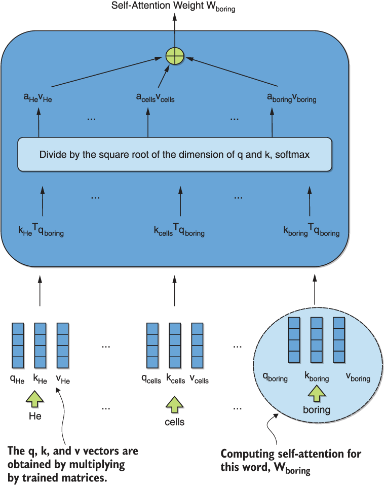
Figure 7.4 A visualization of the calculation of the self-attention weight of the word boring in our example sentence. Observe that the computations of these weights for different words can be carried out independently once key, value, and query vectors have been created. This is the root of the increased parallelizability of transformers over recurrent models. The attention coefficients are what is visualized as intensity of shading in any given column of the multihead attention in figure 7.3.
Each word is associated with a query vector (q), a key vector (k), and a value vector (v). These are obtained by multiplying the input embedding vectors by three matrices that are learned during training. These matrices are fixed across all input tokens. As shown in the figure, the query vector for the current word boring is used in a dot product with each word’s key vector. The results are scaled by a fixed constant—the square root of the dimension of the key and value vectors—and fed to a softmax. The output vector yields the attention coefficients that indicate the strength of the relationship between the current token “boring” and every other token in the sequence. Observe that the entries of this vector indicate the strength of the shadings in any given single column of the multihead attention we visualized in figure 7.3. We duplicate figure 7.3 next for your convenience, so you can inspect the variability in shadings between the various lines.
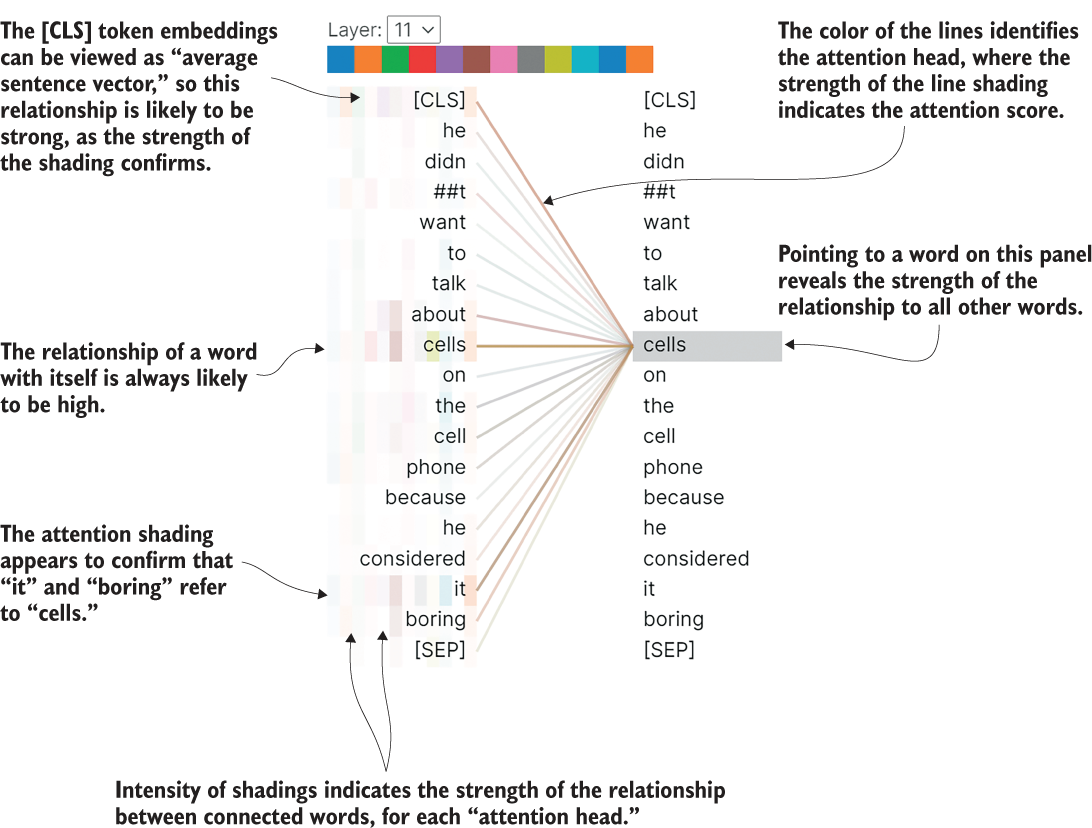
Figure 7.3 (Duplicated) Self-attention visualization in the final encoding layer of the pretrained uncased BERT model for our example sentence. It reveals that “cells” is associated with “it” and “boring.” Note that this is a multihead view, with the shadings in each single column representing each head.
We are now in a good position to understand why transformers are more parallelizable than recurrent models. Recall from our presentation that the computations of self-attention weights for different words can be carried out independently, once the key, value, and query vectors have been created. This means that for long input sequences, one can parallelize these computations. Recall that recurrent models are inherently sequential—the internal hidden state at any given position t depends on the hidden state at the previous position t-1. This means that parallelization of the processing of a long input sequence is not possible in recurrent models because the steps have to be executed one after the other. Parallelization across such input sequences, on the other hand, quickly runs into GPU memory limitations. An additional advantage of transformers over recurrent model is the increased interpretability afforded by attention visualizations, such as the one in figure 7.3.
Note that the computation of the weight for every token in the sequence can be carried out independently, although some dependence between computations exists through the key and value vectors. This means that we can vectorize the overall computation using matrices as shown in figure 7.5. The matrices Q, K, and V in that equation are simply the matrices made up of query, key and value vectors stacked together as matrices.

Figure 7.5 Vectorized self-attention calculation for the whole input sequence using matrices
What exactly is the deal with multihead attention? Now that we have presented self-attention, we are at a good point to address this. We have implicitly been presenting multihead attention as a generalization of self-attention from a single column, in the sense of the shadings in figure 7.3, to multiple columns. Let’s think about what we were doing when we very looking for the noun which “boring” refers to. Technically, we were looking for a noun-adjective relationship. Assume we had one self-attention mechanism that tracked that kind of relationship. What if we also needed to track subject-verb relationships? What about all other possible kinds of relationships? Multihead attention essentially addresses that by providing multiple representation dimensions, not just one.
7.1.3 Residual connections, encoder-decoder attention, and positional encoding
The transformer is a complex architecture with many features that we will not cover in as much detail as self-attention. Mastery of these details is not critical for you to begin applying transformers to your own problems. Therefore, we only briefly summarize them here and encourage you to delve into the original source material to deepen your knowledge over time as you gain more experience and intuition.
As a first such feature, we note that the simplified encoder representation in figure 7.2 does not show an additional residual connection between each self-attention layer in the encoder and a normalization layer that follows it. This is illustrated in figure 7.6.
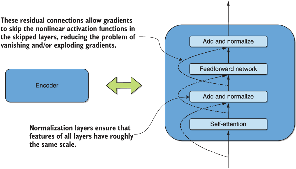
Figure 7.6 A more detailed and accurate breakdown of each transformer encoder, now incorporating residual connections and normalization layers
As shown in the figure, each feedforward layer has a residual connection and a normalization layer after it. Analogous statements are true for the decoder. These residual connections allow gradients to skip the nonlinear activation functions within the layers, alleviating the problem of vanishing and/or exploding gradients. Put simply, normalization ensures that the scale of input features to all layers are roughly the same.
On the decoder side, recall from figure 7.2 the existence of the encoder-decoder attention layer, which we have not yet addressed. We duplicate figure 7.2 next and highlight this layer for your convenience.
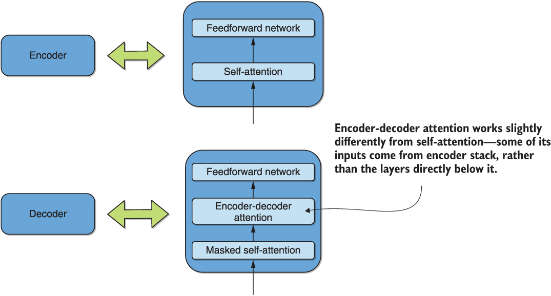
Figure 7.2 (Duplicated, encoder-decoder attention highlighted) Simplified decomposition of the encoder and decoder into self-attention, encoder-decoder attention, and feedforward neural networks
It works analogously to the self-attention layer as described. The important distinction is that the input vectors to each decoder that represent keys and values come from the top of the encoder stack, whereas the query vectors come from the layer immediately below it. If you go through figure 7.4 again with this updated information in mind, you should find it obvious that the effect of this change is to compute attention between every output token and every input token, rather than between all tokens in the input sequence as was the case with the self-attention layer. We duplicate figure 7.4 next—adjusting it slightly for the encoder-decoder attention case—so you can convince yourself.

Figure 7.4 (Duplicated, slightly adjusted for encoder-decoder attention calculation) A visualization of the calculation of the encoder-decoder attention weight between the word boring in our example sentence and the output at position n. Observe that the computations of these weights for different words can be carried out independently once key, value, and query vectors have been created. This is the root of the increased parallelizability of transformers over recurrent models.
On both the encoder and decoder sides, recall from figure 7.1 the existence of the positional encoding, which we now address. Because we are dealing with sequences, it is important to model and retain the relative positions of each token in each sequence. Our description of the transformer operation so far has not touched on “positional encoding” and has been agnostic to the order in which the tokens are consumed by each self-attention layer. The positional embeddings address this, by adding to each token input embedding a vector of equal size that is a special function of the token’s position in the sequence. The authors used sine and cosine functions of frequencies that are position-dependent to generate these positional embeddings.
This brings us to the end of the transformers architecture exposition. To make things concrete, we conclude this section by translating a couple of English sentences to a low-resource language using a pretrained encoder-decoder model.
7.1.4 Application of pretrained encoder-decoder to translation
The goal of this subsection is to expose you to a large set of translation models available at your fingertips within the transformers library. The Language Technology Research Group at the University of Helsinki8 has made more than 1,000 pretrained models available. At the time of writing, these are the only available open source models for many low-resource languages. We use the popular Ghanaian language Twi as an example here. It was trained on the JW300 corpus,9 which contains the only existing parallel translated datasets for many low-resource languages.
Unfortunately, JW300 is extremely biased data, being religious text translated by the Jehovah’s Witnesses organization. However, our investigation revealed that the models are of decent quality as an initial baseline for further transfer learning and refinement. We do not explicitly refine the baseline model on better data here, due to data-collection challenges and the lack of existing appropriate datasets. However, we hope that taken together with the penultimate section of the next chapter—where we fine-tune a multilingual BERT model on monolingual Twi data—you will gain a powerful set of tools for further cross-lingual transfer learning research.
Without further ado, let’s load the pretrained English-to-Twi translation model and tokenizer using the following code:
from transformers import MarianMTModel, MarianTokenizer

model = MarianMTModel.from_pretrained("Helsinki-NLP/opus-mt-en-tw")
tokenizer = MarianTokenizer.from_pretrained("Helsinki-NLP/opus-mt-en-tw")
The MarianMTModel class is a port of encoder-decoder transformer architecture from the C++ library MarianNMT.10 Note that you can change the source and target languages by simply changing the language codes en and tw to representative codes, if made available by the research group. For instance, loading a French-to-English model would change the input configuration string to Helsinki-NLP/opus-mt-fr-en.
If we were chatting with a friend in Ghana online and wanted to know how to write “My name is Paul” by way of introduction, we could use the following code to compute and display the translation:
text = "My name is Paul"                                      ❶
inputs = tokenizer.encode(text, return_tensors="pt")          ❷
outputs = model.generate(inputs)                              ❸
decoded_output = [tokenizer.convert_ids_to_tokens(int(outputs[0][i])) for i in range(len(outputs[0]))]                               ❹
print("Translation:")                                         ❺
print(decoded_output)
❶ Inputs the English sentence to be translated
❷ Encodes to the input token Ids
❸ Generates the output token Ids
❹ Decodes the output token IDs to actual output tokens
The resulting output from running the code is shown next:
Translation:
['<pad>', '▁Me', '▁din', '▁de', '▁Paul']
The first thing we immediately notice is the presence of a special token <pad> in the output that we have not seen before, as well as underscores before each word. This is different from the output the BERT tokenizer produced in section 7.1.1. The technical reason is that BERT uses a tokenizer called WordPiece, whereas our encoder-decoder model here uses SentencePiece. Although we do not get into the detailed differences between these tokenizer types here, we do use this opportunity to warn you once again to review documentation about any new tokenizer you try.
The translation “Me din de Paul” happens to be exactly right. Great! That wasn’t too hard, was it? However, repeating the exercise for the input sentence “How are things?” yields the translation “Ɔkwan bɛn so na nneɛma te saa?” which back-translates literally into “In which way are things like this?” We can see that while the semantics of this translation appear close, the translation is wrong. The semantic similarity, however, is a sign that this model is a good baseline that could be improved further via transfer learning, if good parallel English-Twi data were available. Moreover, rephrasing the input sentence to “How are you?” yields the correct translation “Wo ho te dɛn?” from this model. Overall, this result is very encouraging, and we hope that some readers are inspired to work to extend these baseline models to some excellent open source transformer models for some previously unaddressed low-resource languages of choice.
We look at the Generative Pretrained Transformer (GPT) next, a transformer-based model preferred for text generation that has become quite famous in the NLP community.
7.2 The Generative Pretrained Transformer
The Generative Pretrained Transformer11 (GPT) was developed by OpenAI and was among the earliest models to apply the transformer architecture to the semisupervised learning scenario discussed in this book. By this, we mean, of course, the unsupervised (or self-supervised) pretraining of a language-understanding model on a large corpus of text data, followed by supervised fine-tuning on the final target data of interest. The authors found the performance on four types of language-understanding tasks to be significantly improved. These tasks included natural language inference, question answering, semantic similarity, and text classification. Notably, performance on the General Language-Understanding Evaluation (GLUE) benchmark, which includes these along with other difficult and diverse tasks, was improved by more than 5 percentage points.
The GPT model has undergone several iterations—GPT, GPT-2, and, very recently, GPT-3. Indeed, at the time of writing, GPT-3 happens to be one of the largest known pretrained language models, with 175 billion parameters. Its predecessor, the GPT-2, stands at 1.5 billion parameters and was also considered the largest at the time it was released, just a year prior. Before the release of GPT-3 in June 2020, the largest model was Microsoft’s Turing-NLG, which stands at 17 billion parameters and was released in February 2020. The sheer speed of progress on some of these metrics has been mind-blowing, and these records are likely to be made obsolete very soon. In fact, when GPT-2 was initially disclosed, the authors felt that not fully open sourcing the technology was the right thing to do, given the potential for abuse by malicious actors.
Although at the time of its initial release, GPT became the state of the art for most of the aforementioned tasks, it has generally come to be preferred as a text-generation model. Unlike BERT and its derivatives, which have come to dominate most other tasks, GPT was trained with the causal modeling objective (CLM) where the next token is predicted, as opposed to BERT’s masked language modeling (MLM) fill-in-the-blanks-type prediction objective, which we will cover in more detail in the next chapter.
In the next subsection, we briefly describe the key aspects of the GPT architecture. We follow that with an introduction to the pipelines API concept in the transformers library that is used to minimally execute pretrained models for the most common tasks. We do this in the context of applying GPT to the task it has come to excel at—text generation. Like the previous section on the encoder-decoder transformer and translation, we do not explicitly refine the pretrained GPT model on more-specific target data here. However, taken together with the final section of the next chapter—where we fine-tune a multilingual BERT model on monolingual Twi data—you will gain a powerful set of tools for further text-generation transfer learning research.
7.2.1 Architecture overview
You may recall from section 7.1.1, where we visualized BERT self-attention, that BERT is essentially a stacked set of encoders of the original encoder-decoder transformer architecture. GPT is essentially the converse of that, in the sense that it stacks the decoders instead. Recall from figure 7.2 that besides the encoder-decoder attention, the other distinguishing feature of the transformer decoder is that its self-attention layer is “masked,” that is, future tokens are “masked” when computing attention for any given token. We duplicate figure 7.2 for your convenience, highlighting this masked layer.
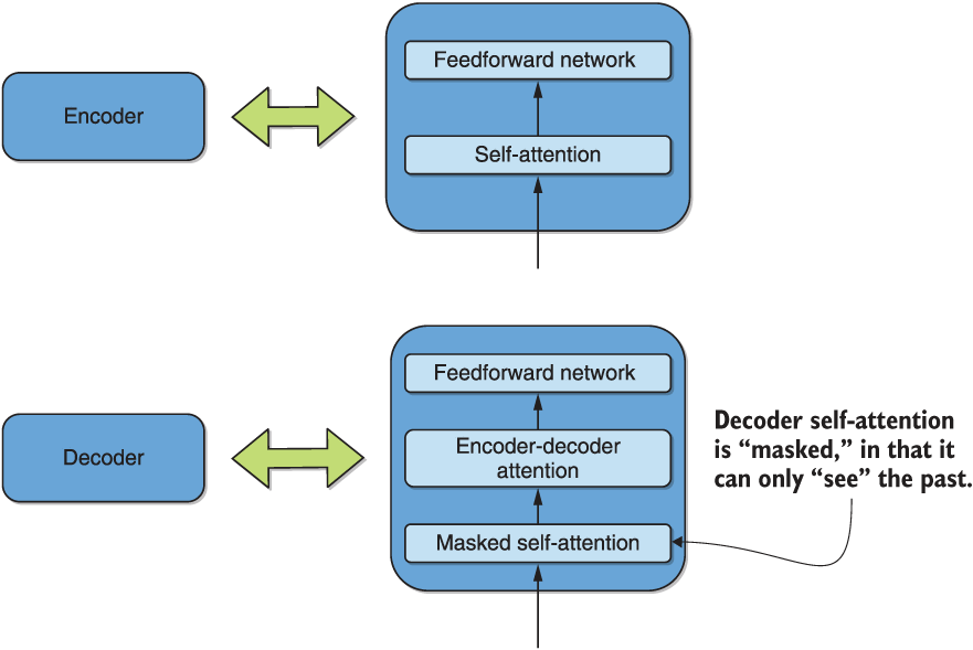
Figure 7.2 (Duplicated, masked layer highlighted) The simplified decomposition of the encoder and decoder into self-attention, encoder-decoder attention, and feedforward neural networks
In the attention calculation that we went through in figure 7.3, this just means including only the tokens in “he didnt want to talk about cells” in the calculation and ignoring the rest. We duplicate figure 7.3 next, slightly modified so you can clearly see the future tokens being masked.

Figure 7.3 (Duplicated again, modified for masked self-attention) A masked self-attention visualization for our example sentence, showing future tokens being masked for causality.
This introduces a sense of causality into the system and suitability for text generation, or predicting the next token. Because there is no encoder, the encoder-decoder attention is also dropped. Taking these factors into account, we show the GPT architecture in figure 7.7.
Note in figure 7.7 that the same output can be used for both text prediction/ generation and classification for some other task. Indeed, the authors devised an input transformation scheme where multiple tasks could be handled by the same architecture without any architectural changes. For instance, consider the task of textual entailment, which roughly corresponds to determining if one premise statement implies another hypothesis statement. The input transformation concatenates the premise and hypothesis statements, separated by a special delimiter token, and feeds the resulting single contiguous string to the same unmodified architecture to classify whether or not entailment exists. On the other hand, consider the important question-answering application. Here, given some context document, a question, and a set of possible answers, the task is to determine which answer is the best potential answer to the question. Here, the input transformation is to concatenate the context, question, and each possible answer before passing each resulting contiguous string through the same model and performing a softmax over the corresponding outputs to determine the best answer. A similar input transformation was devised for the sentence similarity task as well.

Figure 7.7 A high-level representation of the GPT architecture, showing stacked decoders, input embeddings, and positional encodings. The output from the top can be used for both text prediction/generation and classification.
Having briefly introduced the architecture of GPT, let’s use a pretrained version of it for some fun coding experiments. We first use it to generate some open-ended text given a prompt. We then also use a modification of GPT built at Microsoft—DialoGPT12—to perform multiturn conversations with a chatbot in the next subsection.
7.2.2 Transformers pipelines introduction and application to text generation
The first thing we will do in this subsection is generate some open-ended text using GPT. We will also use this opportunity to introduce pipelines—an API exposing the pretrained models in the transformers library for inference that is even simpler than what we did for translation in section 7.1.4. The stated goal of the transformers authors is for this API to abstract away complex code for some frequently used tasks, including named entity recognition, masked language modeling, sentiment analysis, and question answering. Suitably for our purposes in this subsection, text generation is also an option.
Let’s start by initializing the transformers pipeline to the GPT-2 model via the following two lines of code:
from transformers import pipeline
gpt = pipeline('text-generation',model='gpt2')
By way of reminder, GPT in its original form is well suited for open-ended text generation, such as creative writing of sections of text to complement previous text. Let us see what the model generates when primed by “Somewhere over the rainbow...,” up to a maximum of 100 tokens, via the following command:
gpt("Somewhere over the rainbow", max_length=100)
This generates the following text:
[{'generated_text': "Somewhere over the rainbow people live! I wonder how they get to know each other... They just have a wonderful community out there - but when they see each other as two of the best in school they never even realize them, just love, family, friends, and friends. I'm really proud of their talent and dedication to life. I've seen a lot of people that were raised by their mother and grandma in the Midwest and didn't understand there was such an opportunity and I truly cannot"}]
This seems very semantically correct, even if the message is a bit incoherent. You could imagine a creative writer using this to generate ideas to get around writer’s block! Now, let’s see if we can prime the model with something less “creative,” something more technical, to see how it will do. Let’s prime the model with the text “Transfer learning is a field of study” via the following code:
gpt("Transfer learning is a field of study", max_length=100)
This produces the following output:
[{'generated_text': "Transfer learning is a field of study that has been around for centuries, and one that requires a thorough grounding in mathematics in order to understand the complexities of these systems. If you go to the library for your high school physics course, you know you're on the right track. The only problem with this position is that people don't ask questions. The only thing they really do ask is: how do we figure out how to apply these processes to the rest of physics and other sciences?

In"}]
Again, we can see this text is pretty good in terms of semantic coherence, grammatic structure, spelling, punctuation, and so on—indeed, eerily good. However, as it continues, it becomes arguably factually incorrect. We can all agree that transfer learning requires a thorough grounding in mathematics for true understanding and even argue that it has been around for centuries—via us, the humans! However, it is not a field of physics, even if it might be somewhat similar in terms of the kinds of skills required to master it. We can see that the model’s output becomes less plausible the longer it is allowed to speak.
Please be sure to experiment some more to get a sense of the model’s strengths and weaknesses. For instance, you could try prompting the model with our example sentence, “He didn’t want to talk about cells on the cell phone because he considered it boring.” We found this a plausible application in the creative writing space and perhaps in technical writing space with max_length set to a smaller number. It is already a plausible aid for many authors out there. One can only imagine what GPT-3, which has not yet been fully released to the public at the time of writing, will be able to do. The future is indeed very exciting.
Having played around with text generation, let us see if we can use it somehow to create a chatbot.
7.2.3 Application to chatbots
It seems intuitively that one should be able to adopt GPT without major modification to this application. Luckily for us, the folks at Microsoft already did this via the model DialoGPT, which was also recently included in the transformers library. Its architecture is the same as GPT’s, with the addition of special tokens to indicate the end of a participant’s turn in a conversation. After seeing such a token, we can add the new contribution of the participant to the priming context text and iteratively repeat the process via direct application of GPT to generate a response from our chatbot. Naturally, the pretrained GPT model was fine-tuned on conversational text to make sure the response would be appropriate. The authors used Reddit threads for the fine-tuning.
Let’s go ahead and build a chatbot! We will not use pipelines in this case, because this model isn’t yet exposed through that API at the time of writing. This allows us to juxtapose the different methods of calling these models for inference, which is a useful exercise for you to go through.
The first thing to do is load the pretrained model and tokenizer via the following commands:
from transformers import GPT2LMHeadModel, GPT2Tokenizer      ❶
import torch                                                 ❷

tokenizer = GPT2Tokenizer.from_pretrained("microsoft/DialoGPT-medium")
model = GPT2LMHeadModel.from_pretrained("microsoft/DialoGPT-medium")
❶ Note that the DialoGPT model uses the GPT-2 class.
❷ We use Torch here, rather than TensorFlow, because that is the default platform choice in transformers documentation.
A few things are worth highlighting at this stage. First, note that we are using the GPT-2 model classes, which is consistent with our earlier discussion that described DialoGPT as a direct application of that architecture. Additionally, note that we could have used the classes AutoModelWithLMHead and AutoTokenizer interchangeably with these GPT-specific model classes. These utility classes detect the best classes to load the model that is specified by their input strings—in this case, they would detect that the best classes to use were GPT2LMHeadModel and GPT2Tokenizer. You are likely to run across these utility classes as you peruse the transformers library documentation, and it is good to be aware of their existence because they can make your code more general. Finally, note that the “LMHead” version of the GPT is used here. This means that the output from the vanilla GPT is passed through one linear layer and one normalization layer, followed by a transformation into a vector of probabilities of a dimension equal to the size of the vocabulary. The maximum value corresponds to the next most likely token if the model is correctly trained.
The code for conversing with our loaded, pretrained DialoGPT model is shown in listing 7.1. We first specify a maximum number of responses of five. We then encode the conversational contribution of the user at each turn, append the contribution to the chat history, and feed that to the loaded pretrained DialoGPT model for generating the next response.
Listing 7.1 Conversing with the pretrained DialoGPT model for up to five chatbot responses
conversation_length = 5                                                                                           ❶
for step in range(conversation_length):
    new_user_inputs_ids = tokenizer.encode(input("User: ") + tokenizer.eos_token, return_tensors='pt')            ❷
    bot_input_ids = torch.cat([chat_history_ids, new_user_inputs_ids], dim=1)                                     ❸
     if step > 0 else new_user_inputs_ids
    chat_history_ids = model.generate(bot_input_ids, max_length=1000, pad_token_id=tokenizer.eos_token_id)        ❹
    print("DialoGPT: {}".format(tokenizer.decode(chat_history_ids[:, bot_input_ids.shape[-1]:][0], skip_special_tokens=True)))               ❺
❷ Encodes new user input, adds an end-of-sentence token, and returns Tensor
❸ Adds new input to the chat history
❹ Generates a response of up to max_length tokens with chat history as context
One could easily play with this bot all day! We had a lot of fun asking it various questions and prompting it in various ways. We include one such exchange here for your amusement:
User: Hi there.
DialogGPT: Hi there.
User: How are you today?
DialogGPT: I'm good, how are you?
User: Good! How much money do you have?
DialogGPT: I have about 100k.
User: What will you spend it on?
DialogGPT: I'm not sure, I'm not sure what I want to spend it on.
User: Make a decision, life is short.
DialogGPT: I'm going to go with a lot of things.
It’s quite plausible that the entity at the other end of this short conversation is a human, isn’t it? Does that mean it passes the Turing test? Not quite, as the following exchange illustrates:
User: Hi robot.
DialogGPT: Hello, human.
User: Huh?
DialogGPT: I'm a bot.
User: OK, what is your name?
DialogGPT: Robot. I'm a robot.
User: All right then.
DialogGPT: Robot. I'm a robot.
User: Say something else.
DialogGPT: Robot. I'm a robot.
As you increase the number of allowable conversational turns, you will find the bot getting stuck in repeated responses that are off-topic. This is analogous to the GPT open-ended text generation becoming more nonsensical as the length of generated text increases. One simple way to improve this is to keep a fixed local context size, where the model is prompted with conversation history only within that context. Of course, this means the conversation will not always take the context of the entire conversation into account—a trade-off that has to be explored experimentally for any given application.
It is exciting to ponder how well GPT-3 will do on some of these problems, isn’t it? In the final chapter of this book, we will briefly discuss GPT-3 in more detail and introduce a recent smaller but worthy open source alternative to it: GPT-Neo from EleutherAI. It is already available in the transformers library and can be used directly by setting the model string to one of the model names provided by EleutherAI.13 We also include a companion notebook showing it in action for the exercise we performed in this chapter. Upon inspection, you should find its performance better but naturally at a significantly higher cost (the weights of the largest model are more than 10 GB in size!).
We take a look at arguably the most important member of the transformer family—BERT—in the next chapter.
Summary
-
The transformer architecture uses self-attention to build bidirectional context for understanding text. This has enabled it to become a dominant language model in NLP recently.
-
The transformer allows tokens in a sequence to be processed independently of each other. This achieves greater parallelizability than bi-LSTMs, which process tokens in order.
-
The transformer is a good choice for translation applications.
-
The Generative Pretrained Transformer uses the causal modeling objective during training. This makes it the model of choice for text generation, such as chatbot applications.
1. A. Vaswani et al., “Attention Is All You Need,” NeurIPS (2017).
2. A. Radford et al., “Improving Language Understanding by Generative Pre-Training,” arXiv (2018).
3. M. E. Peters et al., “BERT: Pre-Training of Deep Bidirectional Transformers for Language Understanding,” Proc. of NAACL-HLT (2019).
4. https://github.com/google-research/bert/blob/master/multilingual.md
5. A. Radfordet al., “Improving Language Understanding by Generative Pre-Training,” arXiv (2018).
6. A. Vaswaniet al., “Attention Is All You Need,” NeurIPS (2017).
7. https://github.com/jessevig/bertviz
8. https://huggingface.co/Helsinki-NLP
9. http://opus.nlpl.eu/JW300.php
10. https://marian-nmt.github.io/
11. A. Radford et al., “Improving Language Understanding by Generative Pre-Training,” arXiv (2018).
12. Y. Zhang et al., “DialoGPT: Large-Scale Generative Pretraining for Conversational Response Generation,” arXiv (2019).
13. https://huggingface.co/EleutherAI