Search in book...
Toggle Font Controls
Create new playlist

Name your new playlist

Playlist description (optional)
Sign In

Email address

Password

Forgot Password?

or

Continue with Facebook

Continue with Google
Sign Up

Full Name

Email address

Confirm Email Address

Password

or

Continue with Facebook

Continue with Google

Chapter 1

Introduction to CFD

Abstract

This chapter is an introduction to Computational Fluid Dynamics (CFD). Many organizations implement CFD in the computer-aided engineering phase. However, most of the time, higher management is not interested, perhaps because of the lengthy simulations or uncertainty regarding results. These issues are discussed and various misconceptions about CFD are explored and cleared up. The basics of CFD with governing equations are also discussed.

Keywords

CFD; Governing equations; Simulations; Uncertainty

1. Colorful Dynamics or Computational Fluid Dynamics?

Computational fluid dynamics (CFD) is one of the most quickly emerging fields in applied sciences. When computers were not mature enough to solve large numerical problems, two methods were used to solve fluid dynamics problems: analytical and experimental. Analytical methods were limited to simplified cases such as solving one-dimensional (1D) or 2D geometry, 1D flow, and steady flow. However, experimental methods demanded a lot of resources such as electricity, expensive equipment, data monitoring, and data post-processing. Sometimes for engineering analysis work, it is not within the budget of a small organization to establish such a facility. However, with the advent of modern computers and supercomputers, life has become much easier. With the passage of time numerical methods got matured and are now used to solve complex fluid dynamics problems in a short time. Thus, today, with a small investment, some good configuration personal computers can be bought and used to run CFD code that can handle complex flow geometries easily. The results can be achieved more quickly if some of the computers are joined or clustered together.

From an overall perspective, CFD is more economical than experiments. The twentieth century has seen the computer age move with cutting-edge changes, and problems or experiments that had never been thought possible to be performed experimentally or were difficult to perform because of limited resources are now possible with the modern technology. It can be said that CFD is more economical than experiments. With the advent of modern computer technology, it has gained in popularity as well because advanced methods for solving fluid dynamics equations can be analyzed quickly and efficiently.

In terms of accuracy, CFD lies in between the domain of theory and experiments. Because experiments mostly replicate real phenomena, they are much reliable. Analytical method is second because of certain assumptions involved while solving a particular problem. CFD is last because of it involves truncation errors, rounding off errors, and machine errors in numerical methods. To avoid making it “colorful dynamics,” it is the responsibility of the CFD analyst to fully understand the logic of the problem and correctly interpret results.

There are many benefits to performing CFD for a particular problem. A typical design cycle now contains two and four wind-tunnel tests of wing models instead of the 10–15 that were once routine. Because our main focus is High-Performance Computing (HPC), we can say that if CFD is the rider, HPC is the ride. Through HPC complex simulations (such as very high-speed flow) are possible that otherwise would have required extreme conditions for a wind tunnel. For hypersonic flow in the case of a re-entry vehicle, for example, the Mach number is 20 and CFD is the only viable tool with which to see flow behavior. For these vehicles, which cross the thin and upper atmosphere levels, nonequilibrium flow chemistry must be used.

Consider the example of a jet engine whose entire body is filled with complex geometries, faces, and curvature. CFD helps engineers design the after-burner mixers, for example, which provide additional thrust for greater maneuverability. Also, it is helpful in designing nacelles, bulbous, cylindrical engine cowlings, and so forth.

2. Clearing Misconceptions about CFD

An obvious question is why so many CFD users seem unhappy. Sometimes the problem lies in beliefs regarding CFD. Many organizations do not place value on CFD and rely on experiments. According to their view, the use of experiments is customary even though experiments are also prone to errors.

In addition, CFD has captured the research market quicker than experiments owing to the worldwide economic crisis, and it is the obvious choice over experiments for a company when a sufficient budget is scarce. It is also unfortunate that many people do not trust CFD, including the heads of companies and colleagues who sometimes do not understand the complexity of fluid dynamics problems. The analyst must first dig for errors, if any, and then examine how he or she should portray it to higher management. If management is spending money buying expensive hardware and software and hiring people, the importance of CFD is clear. If management still does not recognize the importance of CFD facts, it becomes the job of analysts to educate and mentor the bosses. If it is desired that the statements/arguments related to CFD remain unquestioned, they must be provided either with some scientific or mathematical proof or with some acknowledgment by those who have understanding and firm believe in the truth of the results.

One should compromise for less reliable CFD results when it is known that not enough computational resources are available. This brings us to a question regarding the control of uncertainties. Certain numerical schemes result in dissipation error, such as first order. Other schemes such as second-order result in dispersion error. Then there is machine error, grid accuracy error, human error, and truncation error, to name a few. Thus, unexpected predictions could cause the question, “Did I do something wrong?.” In this case, it is essential to familiarize the user completely with CFD tool(s) and avoid allowing him or her to use the tool as a black box.

Many engineers do not pursue product development, design, and analysis as deeply as do CFD engineers. They do not understand turbulence modeling, convergence, mesh, and such. To sell something in the market using CFD, one should be smart and clever enough to say something the customer can understand.

It is also annoying when software does not correspond the way it should. This occurs when results do not converge or when there is some complex mesh to deal with. At first, one should:

1. Carefully make assumptions if required.

2. Try to make the model simpler (such as using a symmetric or periodic boundary condition).

3. Use reasonable boundary conditions. With an excellent mesh, results do not converge mostly owing to incorrect boundary conditions.

4. Monitor convergence.

5. If not satisfied, go to mesh.

6. If experimental data are unavailable, perform a grid convergence study.

In this way, the efforts will not change skeptics' perceptions overnight but if a history of excellent CFD solutions is delivered, they will start to believe it.

Although CFD has been criticized, there are many great things about it. A CFD engineer enjoys writing code and obtaining results, which increases his confidence level. From a marketing point of view, people are mostly attracted to the colorful pictures of CFD, which is how one can make a presentation truly overwhelming. If one can produce good results but cannot present the work convincingly, then all of the effort is useless.

From this discussion, it can be concluded that there are two important points to remember. One is that the problem does not lie in CFD but could be in the limitation of resources, lack of experimental data, or wrong interpretation of results. Second, skepticism regarding CFD exists but one should be smart enough to present the results in an attractive and evocative manner. Remember the saying that a drop falling on a rock over a long time can create a hole in it. That philosophy will definitely work here, as well. CFD can be colorful dynamics or computational fluid dynamics with colorful, meaningful results. It is your choice: What do you want to see and what do you see?

3. CFD Insight

CFD mainly deals with the numerical analysis of fluid dynamics problems, which embodies differential calculus. The equations involved in fluid dynamics are Navier–Stokes equations. Until now, solutions to Navier–Stokes equations have not been explicitly found except for some cases such as Poiseuille flow, Couette flow, and Stokes flow with certain assumptions. Therefore, several engineers and scientists have spent their lives devising methods to solve these differential equations so as to give a meaningful solution for a particular set of geometry and initial conditions. Thus, CFD is the process of converting the partial differential equations of fluid dynamics into simple algebraic equations and then solving them numerically to obtain some meaningful result.

3.1. Comparison with Computational Structure Mechanics

Because it is a numerical tool, CFD relies heavily on experimental or analytical data for validation. In the author's experience, people who are in the field of computational structure mechanics (CSM) using Finite Element Analysis (FEA) codes for structural deformation in solids do not bother much about creating the grid. This is because the field of FEA is more mature than CFD. For example, there are no complex issues to solve such as the boundary layer, so meshing efforts are reduced. No monster exists such as y+, so life is easier.

In addition, CFD and CSM have two features in common: they both require meshing and they both require HPC when the mesh size is increased. In FEA, as the mesh is increased or the number of nodes increases, the size of the matrices to be solved increases. Similarly, when CFD problems are solved, the number of iterations or calculations increases with the number of grid points, which ultimately need more computational power.

3.2. CFD Process

The entire CFD process consists of three stages: pre-processing, solving, and post-processing. These are diagrammed in Figure 1.1.

Figure 1.1 The computational fluid dynamics process.

All three processes are interdependent. As much as 90% of effort is used in the meshing (preprocessing) stage. This requires the user to be dexterous and there must be the idea of creating an understandable topology. The next stage is to solve the governing equations of flow, which is the computer's work. Remember that an error embedded in the mesh will propagate in the solving stage as well, and if you are lucky enough, you may get a converged solution. However, mostly, owing to only one culprit cell, the solution diverges. The next phase after solving equations is post-processing. There, the results of whatever was input and solved are obtained; colorful pictures showing contours are interpreted for product design, development, or optimization. For validation, the results are compared with experimental data. If any experimental data are absent, the grid convergence study better judges the authenticity of the results. In that case, the mesh is refined two or three times, each time solving and getting results, until a never-changing result (asymptotically converged solution) is obtained.

Post-processing has its own delights, and you can impress people by showing flow simulations such as path lines, flow contours, vector plots, flow ribbons, cylinders, and so forth. In unsteady flows, such as for direct numerical simulation (DNS) and large eddy simulation (LES), the iso-surface of Q-criterion or λ-criterion is also shown sometimes. Post-processing software such as Tecplot has the ability to see multiple things simultaneously in a single picture. As examples, the stream line and flow contours are shown simultaneously in Figure 1.2 for Ariane5 base flow [2] and Figure 1.3 [1] shows the flow over a delta wing. There, the iso-surface of constant pressure is shown over the wing, which is colored by the Mach number. An iso-surface is a surface formed by a collection of points with the same value of a property (such as temperature pressure).

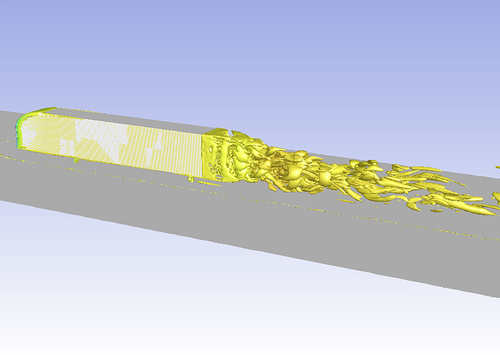
We will focus on turbulent flows in this text because these problems are mostly solved with HPC machines. Turbulence is caused by instabilities in flow and is nondeterministic. There is a range of scales in turbulent flows that can be as large as half the size of the body that causes the turbulence or smaller than one-tenth of a millimeter. In current CFD techniques, in which we use mesh to solve the flow, the mesh size must be such that it contains cells not larger than the size of the smallest scale. Thus, the total mesh size becomes too large for these problems: It could be over 30 million cells. A case for benchmarking such a problem is discussed in Chapter 6, where the mesh size is 111 million cells. The question is where to solve them. That is the purpose of this book, and why we need HPC. HPC solves these problems for us. Figure 1.4 shows an image of the vortices formed behind a truck body. The vortices obviously form as a result of the turbulence in the wake region. A corridor of low velocity often forms behind bodies, called the wake. The scales I was talking about are the length of these vortices, often called eddies. These eddies frequently form and are miscible near the wall of the truck, whereas far from the truck body they mix with outside air and dissipate in the form of heat. If exhaust from the truck is also considered, a more realistic flow would be formed but computationally it would be more complex to solve. An attractive picture of vortices is shown in Figure 1.4.

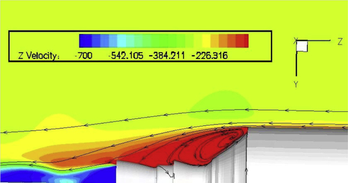
Figure 1.2 Flow structure at the base of Ariane5 ESA Satellite Launch Vehicle [2].

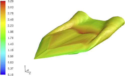
Figure 1.3 Iso-surfaces of pressure colored by the Mach number [1].

Figure 1.4 Eddies form and computed in the wake owing to the technique of Detached Eddy Simulation (DES), which cannot be seen with conventional Reynolds Averaged Navier Stokes (RANS) methods.

3.3. Governing Equations

While we are talking about CFD, the discussion is incomplete without mentioning the governing equations. These equations are the life blood of CFD. The famous equations of fluid dynamics are also known as the Navier–Stokes equation. These equations were discovered independently more than 150 years ago by the French engineer Claude Navier and the Irish mathematician George Stokes. Application of supercomputers to solve these equations introduced the field of CFD. The basis of these equations lies in the assumption that a fluid particle deforms under shear stress. Then, using the second law of motion and energy conservation, the dynamics of the particle is described by its mass, momentum, and energy. In principle, all three parameters must be conserved:

1. Conservation of mass

2. Conservation of momentum

3. Conservation of energy

These set of equations constitute the Navier–Stokes equations. We will not explore the derivation of each of these equations. Instead, the equations are mentioned and complex terms are elaborated.

3.3.1. Conservation of Mass

The conservation of mass equation says that the mass is conserved. It is also known as the continuity equation. The continuity equation is written as:

$\frac{\partial ρ}{\partial t} + \nabla \cdot (ρ \vec{U}) = 0$ $\frac{\partial ρ}{\partial t} + \nabla \cdot (ρ \vec{U}) = 0$

(1.1)

where

$\vec{U} = [u, v, w]$ $\vec{U} = [u, v, w]$

3.3.2. Conservation of Momentum

The conservation of momentum is based on Newton's second law that F = ma, where m is the mass of the fluid particle and a is its acceleration.

When applied to a fluid particle under the action of pressure, viscous and body forces constitute a set of momentum equations. In the x-direction,

$\frac{\partial ρ u}{\partial t} + \frac{\partial ρ u u}{\partial x} + \frac{\partial ρ u v}{\partial y} + \frac{\partial ρ u w}{\partial z} = - \frac{\partial p}{\partial x} + μ \frac{\partial}{\partial x} (\frac{\partial u}{\partial x} + \frac{\partial u}{\partial y} + \frac{\partial u}{\partial z}) + ρ f_{x}$ $\frac{\partial ρ u}{\partial t} + \frac{\partial ρ u u}{\partial x} + \frac{\partial ρ u v}{\partial y} + \frac{\partial ρ u w}{\partial z} = - \frac{\partial p}{\partial x} + μ \frac{\partial}{\partial x} (\frac{\partial u}{\partial x} + \frac{\partial u}{\partial y} + \frac{\partial u}{\partial z}) + ρ f_{x}$

(1.2a)

In the y-direction,

$\frac{\partial ρ v}{\partial t} + \frac{\partial ρ v u}{\partial x} + \frac{\partial ρ v v}{\partial y} + \frac{\partial ρ v w}{\partial z} = - \frac{\partial p}{\partial y} + μ \frac{\partial}{\partial y} (\frac{\partial v}{\partial x} + \frac{\partial v}{\partial y} + \frac{\partial v}{\partial z}) + ρ f_{y}$ $\frac{\partial ρ v}{\partial t} + \frac{\partial ρ v u}{\partial x} + \frac{\partial ρ v v}{\partial y} + \frac{\partial ρ v w}{\partial z} = - \frac{\partial p}{\partial y} + μ \frac{\partial}{\partial y} (\frac{\partial v}{\partial x} + \frac{\partial v}{\partial y} + \frac{\partial v}{\partial z}) + ρ f_{y}$

(1.2b)

and in the z-direction,

$\frac{\partial ρ w}{\partial t} + \frac{\partial ρ w u}{\partial x} + \frac{\partial ρ w v}{\partial y} + \frac{\partial ρ w w}{\partial z} = - \frac{\partial p}{\partial z} + μ \frac{\partial}{\partial z} (\frac{\partial w}{\partial x} + \frac{\partial w}{\partial y} + \frac{\partial w}{\partial z}) + ρ f_{z}$ $\frac{\partial ρ w}{\partial t} + \frac{\partial ρ w u}{\partial x} + \frac{\partial ρ w v}{\partial y} + \frac{\partial ρ w w}{\partial z} = - \frac{\partial p}{\partial z} + μ \frac{\partial}{\partial z} (\frac{\partial w}{\partial x} + \frac{\partial w}{\partial y} + \frac{\partial w}{\partial z}) + ρ f_{z}$

(1.2c)

In 1845, Stokes obtained a relation for the shear stress of Newtonian fluids. With some modification in the viscosity terms, these equations are given as follows:

$τ_{x x} = λ (\nabla \cdot \vec{U}) + 2 μ \frac{\partial u}{\partial x}$ $τ_{x x} = λ (\nabla \cdot \vec{U}) + 2 μ \frac{\partial u}{\partial x}$

(1.2d)

$τ_{y y} = λ (\nabla \cdot \vec{U}) + 2 μ \frac{\partial v}{\partial y}$ $τ_{y y} = λ (\nabla \cdot \vec{U}) + 2 μ \frac{\partial v}{\partial y}$

(1.2e)

$τ_{z z} = λ (\nabla \cdot \vec{U}) + 2 μ \frac{\partial w}{\partial z}$ $τ_{z z} = λ (\nabla \cdot \vec{U}) + 2 μ \frac{\partial w}{\partial z}$

(1.2f)

Asymmetric stress tensors are given as:

$τ_{x y} = τ_{y x} = μ (\frac{\partial v}{\partial x} + \frac{\partial u}{\partial y})$ $τ_{x y} = τ_{y x} = μ (\frac{\partial v}{\partial x} + \frac{\partial u}{\partial y})$

(1.2g)

$τ_{y z} = τ_{z y} = μ (\frac{\partial v}{\partial z} + \frac{\partial w}{\partial y})$ $τ_{y z} = τ_{z y} = μ (\frac{\partial v}{\partial z} + \frac{\partial w}{\partial y})$

(1.2h)

$τ_{z x} = τ_{z x} = μ (\frac{\partial w}{\partial x} + \frac{\partial u}{\partial z})$ $τ_{z x} = τ_{z x} = μ (\frac{\partial w}{\partial x} + \frac{\partial u}{\partial z})$

(1.2i)

where μ is the dynamics viscosity and λ is the second viscosity coefficient, given by Stokes as:

$λ = - \frac{2}{3} μ$ $λ = - \frac{2}{3} μ$

(1.2j)

3.3.3. Energy Equation

The energy equation is based on the principle that energy is conserved. It is also called the First Law of Thermodynamics. Its general form is given in Eqn (1.3):

$\frac{\partial (ρ E)}{\partial t} + \nabla \cdot (ρ E \vec{U}) = ρ \dot{q} + \frac{\partial}{\partial x} (k \frac{\partial T}{\partial x}) + \frac{\partial}{\partial y} (k \frac{\partial T}{\partial y}) + \frac{\partial}{\partial z} (k \frac{\partial T}{\partial z}) - p \nabla \cdot \vec{U} + λ {(\nabla \cdot \vec{U})}^{2} + μ [2 {(\frac{\partial u}{\partial x})}^{2} + 2 {(\frac{\partial v}{\partial y})}^{2} + 2 {(\frac{\partial w}{\partial z})}^{2} + {(\frac{\partial u}{\partial y} + \frac{\partial v}{\partial x})}^{2} + {(\frac{\partial v}{\partial z} + \frac{\partial w}{\partial y})}^{2} + {(\frac{\partial w}{\partial x} + \frac{\partial u}{\partial z})}^{2}]$ $\frac{\partial (ρ E)}{\partial t} + \nabla \cdot (ρ E \vec{U}) = ρ \dot{q} + \frac{\partial}{\partial x} (k \frac{\partial T}{\partial x}) + \frac{\partial}{\partial y} (k \frac{\partial T}{\partial y}) + \frac{\partial}{\partial z} (k \frac{\partial T}{\partial z}) - p \nabla \cdot \vec{U} + λ {(\nabla \cdot \vec{U})}^{2} + μ [2 {(\frac{\partial u}{\partial x})}^{2} + 2 {(\frac{\partial v}{\partial y})}^{2} + 2 {(\frac{\partial w}{\partial z})}^{2} + {(\frac{\partial u}{\partial y} + \frac{\partial v}{\partial x})}^{2} + {(\frac{\partial v}{\partial z} + \frac{\partial w}{\partial y})}^{2} + {(\frac{\partial w}{\partial x} + \frac{\partial u}{\partial z})}^{2}]$

(1.3)

These three governing equations, i.e., continuity, momentum, and energy, constitute the Navier–Stokes equations. Some authors refer to only momentum equations as Navier–Stokes equations. These equations are important in CFD and the reader should memorize them to understand the methods of CFD. In CFD these equations are discretized along with points in space and then solved algebraically.

To solve these, various approaches are used, such as the finite difference method (FDM), finite volume method (FVM), and finite element method. These equations can be modified for inviscid, incompressible, or compressible and steady or unsteady fluid flow. For an inviscid flow field, the viscous terms would be neglected and the leftover equations would then be referred to as Euler equations.

In theory, the Navier–Stokes equations describe the velocity and pressure of fluid accelerating by any point near the surface of a body. If we consider an aircraft body as an example; these data can be used by engineers to compute, for various flight conditions, all aerodynamic parameters of interest, such as the lift, drag, and moment (twisting forces) exerted on the airplane. Drag is particularly important with respect to the fuel efficiency of an aircraft because it is one of the largest operating expenses for most airlines. It is not surprising that many aircraft companies spend a large amount of money for drag reduction research even if it results in one-tenth of a percent. Computation-wise, drag is the most difficult to compute compared with moment and lift.

To make these equations understandable to a computer, it is essential to represent the aircraft's surface and the space around it in a form that is usable by the computer. To do this, codes are developed in which the aircraft and its surroundings are represented as a series of regularly spaced points called a computational grid. These are then supplied to the solver code that applies Navier–Stokes equations to the grid data. The computer then computes the values of air velocity, pressure, temperature, and so forth, at all points. In effect, the computational grid breaks up the computational problem in space; the calculations are carried out at regular intervals to simulate the passage of time, so the simulation is temporally discretized as well. The closer the gird points are, the more often they will be computed and the more accurate and realistic the simulation is.

The problem is still not straightforward. The Navier–Stokes equations are in fact nonlinear, so many variables in these equations vary with respect to each other by powers of two or greater. Interaction of these nonlinear variables creates newer terms, which makes the solution difficult to solve. In addition, the global dependence of variables augments the complexity, such as the pressure which at a point depends on the flow at many other points. Because the different parts of a single problem are so intermingled, the solution must be obtained at many points simultaneously.

While we are dealing with CFD, keep in mind that our main focus in the CFD area is turbulence. This is because turbulence is currently the door for which HPC is the key. Only computational solutions give a detailed prediction of turbulence, which is not possible through other experimental or analytical means.

4. Methods of Discretization

There are several methods of discretization that are programmed in commercial codes. ANSYS FLUENT and ANSYS CFX both use FVM. This is because FVM has certain advantages and the scheme is robust. The most popular methods are FDM and FVM, and we will discuss them next.

4.1. Finite Difference Method

Of all methods, FDM is the simplest. It can be said that CFD started from FDM. Initially, mathematicians derived simple formulas to calculate derivatives and then the methods improved and CFD advanced to more advanced methods. Currently, computations such as DNS and LES are only theoretical. The rationale of FDM can be understood from the concept of a derivative. The derivative of a function gives the slope of the function. For a function of x-component of velocity u, the slope of u with respect to x can be determined numerically as:

$\frac{\partial u}{\partial x} = \frac{u_{i + 1} - u_{i}}{Δ x}$ $\frac{\partial u}{\partial x} = \frac{u_{i + 1} - u_{i}}{Δ x}$

(1.4)

where the subscripts i and i + 1 are the points for calculating the u values. Here, Δx denotes the grid spacing. The method for calculating the first derivative is also called the forward difference method, as we will soon observe.

4.2. Taylor Series Expansion and Forward Difference

4.2.1. Forward Difference Scheme

All of the derivatives are derived numerically using Taylor series expansion. The number of points used to evaluate the derivative is called the stencil. The higher the number of points is, the more accurate will be the numerical result. Consequently, the spacing reduction between points also improves accuracy, but with some limitations. For a forward difference approximation the stencil would be i and i + 1. Hence, for function u the value at i + 1, i.e., u_i ₊ ₁, would be:

$u_{i + 1} = u_{i} + \frac{\partial u}{\partial x} Δ x + \frac{\partial^{2} u}{\partial x^{2}} {(\frac{Δ x}{2!})}^{2} + \frac{\partial^{3} u}{\partial x^{3}} {(\frac{Δ x}{3!})}^{3} + \dots$ $u_{i + 1} = u_{i} + \frac{\partial u}{\partial x} Δ x + \frac{\partial^{2} u}{\partial x^{2}} {(\frac{Δ x}{2!})}^{2} + \frac{\partial^{3} u}{\partial x^{3}} {(\frac{Δ x}{3!})}^{3} + \dots$

(1.5)

This formulation is then modified to evaluate the derivative. Divide each term by Δx and manipulate the terms:

$\frac{\partial u}{\partial x} = \frac{u_{i + 1} - u_{i}}{Δ x} + O (Δ x)$ $\frac{\partial u}{\partial x} = \frac{u_{i + 1} - u_{i}}{Δ x} + O (Δ x)$

(1.6)

This equation is called the first-order forward difference scheme. The last term, O(Δx), indicates that the formulation is first order. This means that when the Taylor series formula was divided by Δx, the least derivative term containing the Δx term was of the order of 1 (power of 1).

4.2.2. Backward Difference Scheme

The backward difference scheme is as straightforward as the forward difference scheme. The stencil is reversed, i.e., i and i − 1. The Taylor series expansion is:

$u_{i - 1} = u_{i} - \frac{\partial u}{\partial x} Δ x + \frac{\partial^{2} u}{\partial x^{2}} {(\frac{Δ x}{2!})}^{2} - \frac{\partial^{3} u}{\partial x^{3}} {(\frac{Δ x}{3!})}^{3} + \dots$ $u_{i - 1} = u_{i} - \frac{\partial u}{\partial x} Δ x + \frac{\partial^{2} u}{\partial x^{2}} {(\frac{Δ x}{2!})}^{2} - \frac{\partial^{3} u}{\partial x^{3}} {(\frac{Δ x}{3!})}^{3} + \dots$

(1.7)

Divide each term by Δx and manipulate the terms:

$\frac{\partial u}{\partial x} = \frac{u_{i} - u_{i - 1}}{Δ x} + O (Δ x)$ $\frac{\partial u}{\partial x} = \frac{u_{i} - u_{i - 1}}{Δ x} + O (Δ x)$

(1.8)

It should be noted that forward and backward schemes are first-order accurate.

4.2.3. Central Difference Scheme

The central differencing scheme is obtained by combining the forward series and backward series. This is done by subtracting the backward from the forward scheme. Subtracting Eqn (1.7) from Eqn (1.5), the following formulation is obtained:

$\frac{\partial u}{\partial x} = \frac{u_{i + 1} - u_{i - 1}}{2 Δ x} + O (Δ x)$ $\frac{\partial u}{\partial x} = \frac{u_{i + 1} - u_{i - 1}}{2 Δ x} + O (Δ x)$

(1.9)

Figure 1.5 Graphical representation of three basic finite difference schemes.

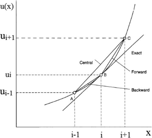
The last term indicates the order of the central difference scheme. The central difference scheme is second-order accurate. Therefore, it is widely used in the calculations. The error that arises owing to the truncation (cutting) of the higher-order derivatives of the Taylor series terms is called the truncation error.

4.2.4. Second-Order Derivative

To obtain the second-order derivative, the method is slightly tedious. Because it involves more and more terms, the equations become more and more complex mathematically. By adding Eqns (1.5) and (1.7), we get:

$\frac{\partial^{2} u}{\partial x^{2}} = \frac{u_{i + 1} - 2 u_{i} + u_{i - 1}}{Δ x^{2}} + O (Δ x^{2})$ $\frac{\partial^{2} u}{\partial x^{2}} = \frac{u_{i + 1} - 2 u_{i} + u_{i - 1}}{Δ x^{2}} + O (Δ x^{2})$

(1.10)

The three methods mentioned above are shown in Figure 1.5.

4.3. Finite Volume Method

The FVM is widely used in CFD codes because of its various advantages over FDM. The FVM can be used for any sort of grid, i.e., structured or unstructured, clustered or non-clustered, and so forth. It can also be used in cases where there is discontinuity in the flow where FDM fails to calculate. In the FVM the computational domain is divided into a number of control volumes. The values are calculated at cell centers. The values of fluxes at the cell interface are determined through interpolation using the values at the cell centers. For each control volume an algebraic equation is obtained, and thus a number of equations appear that are then solved using numerical methods. The FVM should not be confused with geometric volume definition. It has nothing to do with physical volume. Both schemes, i.e., FDM and FVM, can be used in 2D and 3D flow fields.

The term “volume” refers to the fact that, to solve fluid dynamics equations, the domain is discretized using control volumes (which could be 2D, as well) instead of taking discrete points as for the FDM. This is also a paramount reason to accommodate unstructured grids in FVM. One disadvantage of the FVM method is that higher-order schemes greater than second order are difficult to handle in three dimensions. This is because of dual approximations: that is, interpolation between the cell centers and the interfaces and the integration of all surfaces.

4.3.1. Simplest Approach: Gauss's Divergence Theorem

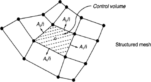
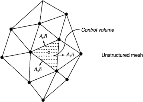
We begin by considering Gauss's divergence theorem for a control volume. The mesh for FVM can be structured or unstructured. Figures 1.6 and 1.7 show the structured and unstructured mesh for FVM. The normal

\bar{n}

$\bar{n}$

represents the vector normal to the surface. The function ϕ can be any perimeter such as velocity, temperature, or pressure. The first-order derivative in x-direction is:

$\frac{\partial ϕ}{\partial x} = \frac{1}{Δ V} \int_{V} \frac{\partial ϕ}{\partial x} d V = \frac{1}{Δ V} \int_{A} ϕ d A^{x} = \frac{1}{Δ V} \sum_{i = 1}^{N} ϕ_{i} A_{i}^{x}$ $\frac{\partial ϕ}{\partial x} = \frac{1}{Δ V} \int_{V} \frac{\partial ϕ}{\partial x} d V = \frac{1}{Δ V} \int_{A} ϕ d A^{x} = \frac{1}{Δ V} \sum_{i = 1}^{N} ϕ_{i} A_{i}^{x}$

(1.11)

where ϕ_i is the variable value at the elemental surfaces and N denotes the number of bounding surfaces on the elemental volume. Equation (1.11) applies for any type of finite volume cell that can be represented within the numerical grid. For the structured mesh shown in Figure 1.6, N has a value of 4 because there are four bounding surfaces of the element. In 3D, for a hexagonal element, N becomes 6. Similarly, the first-order derivative for ϕ in the y-direction is obtained, which can be written as:

$\frac{\partial ϕ}{\partial y} = \frac{1}{Δ V} \int_{V} \frac{\partial ϕ}{\partial y} d V = \frac{1}{Δ V} \int_{A} ϕ d A^{y} = \frac{1}{Δ V} \sum_{i = 1}^{N} ϕ_{i} A_{i}^{y}$ $\frac{\partial ϕ}{\partial y} = \frac{1}{Δ V} \int_{V} \frac{\partial ϕ}{\partial y} d V = \frac{1}{Δ V} \int_{A} ϕ d A^{y} = \frac{1}{Δ V} \sum_{i = 1}^{N} ϕ_{i} A_{i}^{y}$

(1.12)

Figure 1.6 Structured mesh for finite volume method.

Figure 1.7 Unstructured mesh for finite volume method.

Problem

This problem describes the discretization of continuity equation using FVM. The results are shown and compared with the FDM solution of the same equation. The 2D continuity equation must be discretized:

$\frac{\partial u}{\partial x} + \frac{\partial v}{\partial y} = 0$ $\frac{\partial u}{\partial x} + \frac{\partial v}{\partial y} = 0$

(1.13)

on a structured grid.

Figure 1.8 Stencil of finite volume method grid for the problem.

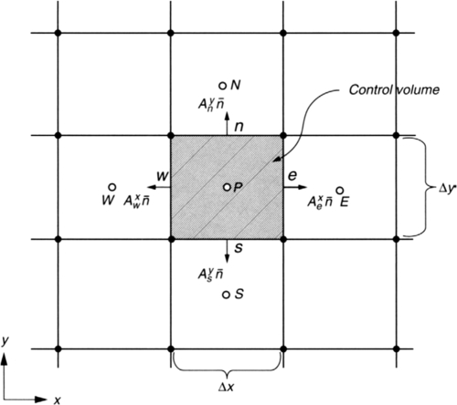
Solution: The stencil used for the problem is shown in Figure 1.8. Introducing control volume integration, that is, applying Eqns (1.11) and (1.12), yields the following expressions, which are applicable to both structured and unstructured grids:

$\frac{\partial ϕ}{\partial x} = \frac{1}{Δ V} \sum_{i = 1}^{N} ϕ_{i} A_{i}^{x} = \frac{u_{e} A_{e}^{x} - u_{w} A_{w}^{x} + u_{n} A_{n}^{x} - u_{s} A_{s}^{x}}{Δ V}$ $\frac{\partial ϕ}{\partial x} = \frac{1}{Δ V} \sum_{i = 1}^{N} ϕ_{i} A_{i}^{x} = \frac{u_{e} A_{e}^{x} - u_{w} A_{w}^{x} + u_{n} A_{n}^{x} - u_{s} A_{s}^{x}}{Δ V}$

(1.14)

Similarly,

$\frac{\partial ϕ}{\partial y} = \frac{1}{Δ V} \sum_{i = 1}^{N} ϕ_{i} A_{i}^{y}$ $\frac{\partial ϕ}{\partial y} = \frac{1}{Δ V} \sum_{i = 1}^{N} ϕ_{i} A_{i}^{y}$

(1.15)

For the structured uniform grid arrangement, the projection areas

A_{n}^{x}

$A_{n}^{x}$

and

A_{s}^{x}

$A_{s}^{x}$

in the x-direction and the projection areas

A_{e}^{y}

$A_{e}^{y}$

and

A_{w}^{y}

$A_{w}^{y}$

in the y-direction are zero. One important aspect demonstrated here by the FVM is that it allows direct discretization in the physical domain (or in a body-fitted conformal grid) without the need to transform the continuity equation from the physical domain to a computational domain as required in the FDM.

Because the grid has been considered to be uniform, face velocities u_e, u_w, v_n, and v_s are located midway between each of the control volume centroids, which allows us to determine the face velocities from the values located at the centroids of the control volumes. This implies:

$u_{e} = \frac{u_{E} + u_{P}}{2}; u_{w} = \frac{u_{P} + u_{W}}{2}; v_{n} = \frac{v_{N} + v_{P}}{2}; v_{s} = \frac{v_{P} + v_{S}}{2}$ $u_{e} = \frac{u_{E} + u_{P}}{2}; u_{w} = \frac{u_{P} + u_{W}}{2}; v_{n} = \frac{v_{N} + v_{P}}{2}; v_{s} = \frac{v_{P} + v_{S}}{2}$

By substituting these expressions into the discretized form of the velocity first-order derivatives, the final form of the discretized continuity equation becomes:

$\frac{u_{E} + u_{P}}{2} A_{e}^{x} - \frac{u_{P} + u_{W}}{2} A_{w}^{x} + \frac{v_{N} + v_{P}}{2} A_{n}^{y} - \frac{v_{P} + v_{S}}{2} A_{s}^{y}$ $\frac{u_{E} + u_{P}}{2} A_{e}^{x} - \frac{u_{P} + u_{W}}{2} A_{w}^{x} + \frac{v_{N} + v_{P}}{2} A_{n}^{y} - \frac{v_{P} + v_{S}}{2} A_{s}^{y}$

Putting this into the above equation and manipulating, we get:

$(\frac{u_{E} - u_{W}}{2 Δ x}) + (\frac{v_{N} - v_{S}}{2 Δ y}) = 0$ $(\frac{u_{E} - u_{W}}{2 Δ x}) + (\frac{v_{N} - v_{S}}{2 Δ y}) = 0$

(1.16)

This is the continuity equation obtained with the FVM. It is interesting to check the results with the FDM. The above formulation has 2Δx and 2Δy in the denominator, which indicates the second-order accuracy of the scheme. If the central difference is used for the continuity equation which discretized just above, a similar formulation will be obtained. Using the stencil of Figure 1.8, the formulation can be made by applying the forward difference between E and P:

$u_{E} = u_{P} + \frac{\partial u}{\partial x} Δ x + \frac{\partial^{2} u}{\partial x^{2}} {(\frac{Δ x}{2!})}^{2} + \frac{\partial^{3} u}{\partial x^{3}} {(\frac{Δ x}{3!})}^{3} + \dots$ $u_{E} = u_{P} + \frac{\partial u}{\partial x} Δ x + \frac{\partial^{2} u}{\partial x^{2}} {(\frac{Δ x}{2!})}^{2} + \frac{\partial^{3} u}{\partial x^{3}} {(\frac{Δ x}{3!})}^{3} + \dots$

(1.17)

and the backward difference between P and W:

$u_{W} = u_{P} - \frac{\partial u}{\partial x} Δ x + \frac{\partial^{2} u}{\partial x^{2}} {(\frac{Δ x}{2!})}^{2} - \frac{\partial^{3} u}{\partial x^{3}} {(\frac{Δ x}{3!})}^{3} + \dots$ $u_{W} = u_{P} - \frac{\partial u}{\partial x} Δ x + \frac{\partial^{2} u}{\partial x^{2}} {(\frac{Δ x}{2!})}^{2} - \frac{\partial^{3} u}{\partial x^{3}} {(\frac{Δ x}{3!})}^{3} + \dots$

(1.18)

Because we know that the central difference is obtained by subtracting the backward from the forward formulation. Subtracting Eqn (1.18) from Eqn (1.17) implies:

$\frac{u_{E} - u_{W}}{2 Δ x}$ $\frac{u_{E} - u_{W}}{2 Δ x}$

(1.19)

Similarly, for the y-component, performing this operation again with N and S cell centers and v as the velocity component, we get:

$\frac{v_{N} - v_{S}}{2 Δ y}$ $\frac{v_{N} - v_{S}}{2 Δ y}$

(1.20)

Summing both Eqns (1.19) and (1.20) and equating to zero to get the continuity equation:

$(\frac{u_{E} - u_{W}}{2 Δ x}) + (\frac{v_{N} - v_{S}}{2 Δ y}) = 0$ $(\frac{u_{E} - u_{W}}{2 Δ x}) + (\frac{v_{N} - v_{S}}{2 Δ y}) = 0$

(1.21)

Comparing Eqn (1.21) with Eqn (1.16), there is no difference between them. Both schemes are second-order accurate.

5. Turbulence Should Not Be Taken for Granted

For a turbulent flow case, the variation in length scales, often represented by the ratio of the largest to the smallest eddy size, can be computed from the Reynolds number raised to the power 3/4. We will see in Chapter 4 that this ratio can be used to calculate the number of cells required for a reasonably accurate simulation. Because a practical problem is 3D, the number of grid points becomes proportional to the Reynolds number raised to the power 9/4. Thus, in simpler terms, doubling the Reynolds number increases the grid points five times.

Let us consider an aircraft that is 50 m long and wings with a chord length (the distance from the leading edge to the trailing edge) of about 5 m. It is cruising at 250 m/s at an altitude of 10 km. For this, 10¹⁶ grid points are needed to simulate turbulence near the surface with sufficient detail [3]. We will explore this in detail in Chapter 4, but for the time being note that currently, even with a supercomputer capable of performing 10¹² floating point operations/second, it would take several thousand years to compute the flow for 1 s of flight.

In fact, engineers are rarely interested about detailed turbulent quantities such as small eddy dissipation; their main concern is usually with mean flow quantities, or in the case of aircraft, the lift and drag forces and heat transfer. In the case of an internal combustion engine (ICE), they could be interested in the rates at which the fuel and oxidizer mix. Including turbulence means including the fluctuating terms in the coupled Navier–Stokes equations. These fluctuating terms are mostly time-averaged, thereby smoothing the flow. This practice dramatically reduces the number of grid points. Some models used to model the terms arise as a result of the averaging procedure in Navier–Stokes. All of the models carry some assumptions and contain coefficients based on experimental findings. Therefore, it would be too good to be true to accept that a turbulent flow simulation could be as good as the model it contains.

6. Technological Innovations

Fluid dynamicists are able to find a way to directly simulate the greater portions of turbulent eddies with the advent of the fast computer era. In this way, there is a compromise between DNS and turbulence-averaged quantities simulation. The compromise has resulted in LES. With this technique, large eddies are resolved while small eddies are modeled. The technique emerged from meteorology, in which the large-scale turbulent motion of clouds was of particular interest. Currently, engineers are able to use the technique widely in other areas of fluid sciences such as for gases inside combustion chambers of ICE. DNSs are no longer theoretical. Simple cases such as pipe flow offer deep insight into turbulence through DNS. These simulations have also helped engineers fine-tune the coefficients used in models of turbulence.

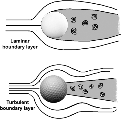
A study was done by P. Moin [3,4] regarding the control of turbulence. The study was conducted on drag reduction for civilian aircraft. The concept of riblets was used, adopted from tooth-like structures on the skin surface of sharks. Numerical simulations using DNS showed that riblets tend to reduce the motion of eddies, preventing them from coming close to the surface of the body (within about 50 μm). This preserves the transportation of a high-speed fluid close to the surface. Another technology that employs this development is active control. Converse to the passive technology of riblets, this technology uses control surfaces to move against the turbulent fluctuations of an incoming fluid. The wing surface contains several micro-electromechanical systems that respond to pressure fluctuations to control the small eddies that cause turbulence. Fluid dynamicists are able to become involved in all of these efforts only by seeing nature in the form of a shark's skin movement. They are trying to build smarter aircrafts using this technique. This drag effect is not limited to aircraft skins; the technology is also used in golf balls. The drag exerted on the ball mostly results from pressure, which is more in front than behind the ball. Golf balls have dimples on their surface that increase turbulence and hence reduce drag, thereby increasing the ability to travel about two and half times farther than a plane-surface ball (Figure 1.9).

Figure 1.9 Flow behind a plane ball and a golf ball, a laminar boundary layer experiences more drag than a turbulent one.

Thus, CFD helps us in many complicated cases for which we cannot easily judge or analyze based on experimental or analytical data. The growing popularity of CFD is solely due to the rapid increase in computational power and the efficacy that is reflected by the field itself. However, because humanity's desires do not rest, as computational power crosses a quadrillion floating-point operations per second, scientists and fluid dynamicists will begin to float new complex problems that are currently thought to be impossible to solve.

..................Content has been hidden....................

You can't read the all page of ebook, please click here login for view all page.

Table of Contents for Chapter 1. Introduction to CFD

Create new playlist

Sign In

Sign Up