The sheer volume of answers can often stifle insight...The purpose of computing is insight, not numbers.
—[2]
Framework
Computers have become one of the main resources for research. They are essential to analyze models through simulations, giving more options to verify the interactions between the components of a model, and essential to analyze large amounts of data.
Simulation is used for theoretical and empirical research since it provides the means to explore all the capacities and limits of theoretical models and because it helps to create synthetic conditions that are difficult to re-create in a real experiment. In some research specialties, this field is considered a third methodology [3]. For instance, any tangible laboratory sample can be re-created with a model in the computing world; the physical device would be the computer program or software, and the measurements would be the computer tasks [4]. A simulation is an application or a computer process that attempts to imitate a physical process by producing a similar response that allows someone to make predictions about the expected behavior of a system. As a result, it can be used as an experimental setup or as a support to make operational decisions. It is also employed to study difficult and complex systems before spending resources on a real experiment.
Simulations, Models, and Their Importance in Research
Before any simulation, it is essential to have a model. It is a conceptual representation of a real system whose level of abstraction depends on the research question and previous knowledge from the system. A simulation cannot be executed by itself, since it requires a tool (programming framework) and a platform (computer, server, etc.) to execute and produce a response. The computational cost of a simulation depends on the complexity of the real system and the level of abstraction used to model it.
Even though some models can be validated using mathematical formalisms, some systems are complex, involving many variables and input parameters that make mathematical validation challenging. For these kinds of models, simulation provides a form of understanding at different levels; however, the knowledge acquired from these models is useful in a limited way, since the behavior is seen in conditions that are difficult to test or that are generally not seen in real systems.
If the theory is accurate, simulation is a great tool to study theoretical models. It also allows discovering how the responses would be in different scenarios. Simulation cannot validate a model by itself, only instantiate it. Therefore, to validate it, the same test scenario must be implemented under real-world conditions to compare its results with the simulation output to gain enough accuracy of the model and validate it.
Theoretical models represent the behavior of the system based on its knowledge and not the behavior of a real system. These models need validation before being considered empirical. An ideal way to validate them is through simulation. When simulating a theoretical model under a determined set of conditions, the result works as a hypothesis for the behavior of the real system if it is tested under the same circumstances. If the experiment data is statistically close to the simulation output, it is feasible to infer that the model is accurate. If the model does not seem satisfactory, it does not imply that there are errors in it. There could be, but there could also be errors in instantiating the model, which could serve as a guideline for telling what not to do for a future experiment. Simulation is a powerful tool. This whole process is a method to validate simulation models through experimentation. However, it is not a substitute for real experimentation, since the simulation results are only as good as the models used. Therefore, it is mandatory to validate the model and question their results and applicability if this has not been done.
The quality of the simulation results is directly associated with the quality of the model. This implies that it is necessary to validate a model before deploying it. Model validation is a process in which the experiment is evaluated if it is an accurate representation from a real system. Empirical studies are used to ensure their accuracy. However, according to the research needs, not every model needs to be validated with the same level of accuracy. In general, to validate a model, it is possible to use two methodologies: observational methods and the experimentation, exposed earlier.
The observational methods are usually aimed at answering the research question, but in the case of simulation models, they are used to ask questions to the model output data to determine its validity. Thanks to machine-learning techniques and statistical methods, it is possible to carry out observation methods. On the one hand, machine-learning techniques employ algorithms that learn distributions and correlations to produce a model from the output data. On the other hand, to ask questions and get answers from the output data, statistical methods are used if the data has a behavior that can match certain distributions.
Types of Simulation Techniques
There are two types of systems: discrete and continuous. In a discrete system, the state variables change instantly at different points in time. On the other hand, in a continuous system, the state variable change continuously over time.
In computer networks, many systems function as discrete systems (LAN, cellular infrastructure, wireless networks); in them, specific events or interactions change the state and the behavior of the entire system. In the simulation program, these events are inserted and read as states, variables, and routines sequentially; this approach is known as next-event time advance. All these attributes and events are enabled in the debugging and execution processes along with the input scripts. The general orientation of the processing is carried out through modeling, which is usually formulated in a general-purpose language.
Types of Simulations
Type of Simulations | Description |
|---|---|
Emulation | This is the process of designing and building a model that uses real system functionality. A study case is the prototyping process. |
Monte Carlo simulation | This is a simulation process without time reference. Monte Carlo simulation techniques are used to model any probabilistic phenomenon that does not change over time as an independent variable. |
Trace-driven simulation | This simulation uses as input an ordered list equivalent to real-world events. In this type of simulation, the time variable is an attribute of the event. |
Continuous-event simulation | A function can model this type of simulation, and the changes occur permanently. An issue is to determinate the scale and the scope of the experiment to identify the factors and events that influence the results. |
Discrete-event simulation (DES) | Discrete event simulation is a type of simulation that uses “events” to specify details of an experiment that occur over time. Discrete mathematical analysis can model the process and have a medium level of abstraction. Each event is a function or class call with a unique identifier. |
Event queue: This contains all the events waiting to happen. The implementation of the event list and the functions to be performed on it can significantly affect the efficiency of the simulation program.
Simulation clock: This is a global variable that represents the simulation time; the simulator advances in the simulation time until the next scheduled event. During event execution, the simulation time is frozen; however, in the ns-3 simulator, it is possible to work with the real-time scheduler integrated with the hardware clock to perform the progression of the simulation clock in a synchronized way with the machine or reference external clock.
State variables: These variables help to describe the state of the system.
Event routines: These routines handle the occurrence of events. Once an event is successfully executed, the simulator updates the state variables and the event queue.
Input routine: This routine obtains the user input parameters and supplies them to the model.
Output generation routine: This routine is in charge of creating the output of the events and the abstraction of the simulator. In ns-3, there are two kinds of outputs: .pcap and .tr files.
Main program: This is the entry point on the ns-3 simulator where it is possible have C++ and Python’s main() function program. The main program is used to call the classes, functions, libraries, and methods useful to execute the simulation. The simulation on ns-3 begins with the Simulator::Run() routine and ends with the Simulator::Destroy() routine.
Formal Systems Concepts
Behavior: This is the relationship between any input/output pair in a system at different times. It can be obtained from external measurement to know the internal set of events and states that characterize the system [6].
Emulation: A partial or complete construction of a system that is functional and artificial, whose behavior mimics that of an analyzed reference system, this is the process of simulating the inner workings of a systems to produce a realistic output [7].
Event: This is the source of the changes in a finite state machine.
Inference: This is an activity oriented to deduce the internal structure of a system from its behavior. (This definition is close to the simulation world.)
Structure: This is an internal characteristic that defines a set of system states and relations [6].
Regarding the real experimenting analogies, when the scope of a simulation process is to imitate a real physical process, it is important to consider an experimental orientation for collecting process data and for data analysis techniques that is similar to a scientific inference laboratory. Otherwise, in computer systems, simulations are sort of hybrid experiments, because just one side of the processes comes from the real world, like propagation media features, transmission lines parameters, delays, failures, and other common behaviors of hardware. The other side consists of software processes.
The creation of different kinds of models is the result of efforts to simulate and imitate real systems. Essentially, real-life systems and phenomena are continuous models, which means that the variables of the process can be set at any time. Unlike real-word systems, computational processing uses discrete models, which are models that change state at certain times and have a limited number of possible states.
In the description of discrete events of a system, there are instantaneous changes of discrete variables that allow imitating a real dynamic system. A combination of differential equation system specifications and discrete event system specification, inherent in the continuous and discrete descriptions respectively, allows the computational models to simulate real systems in an approximate way.
Simulation and Emulation
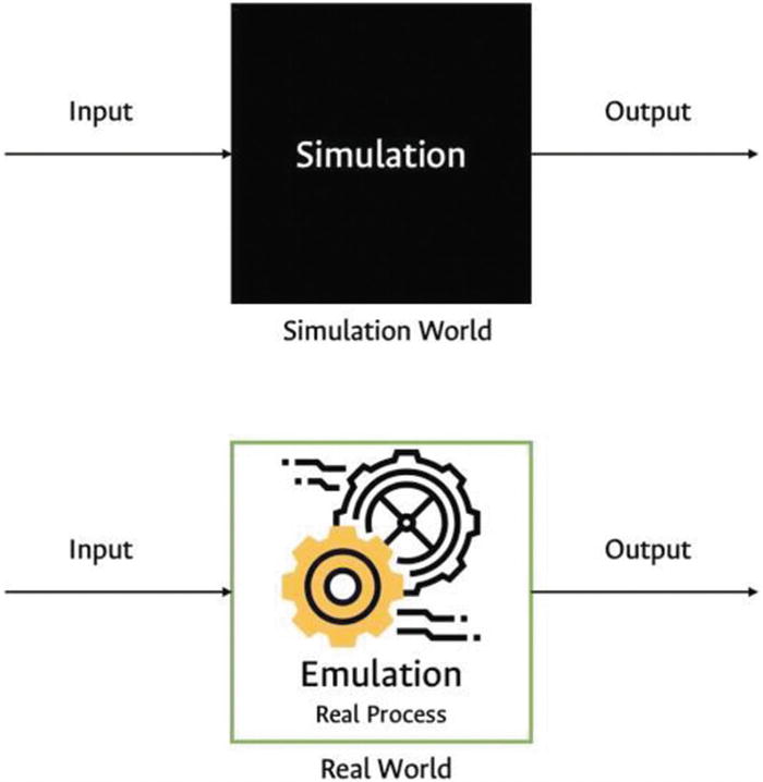
Simulation versus emulation
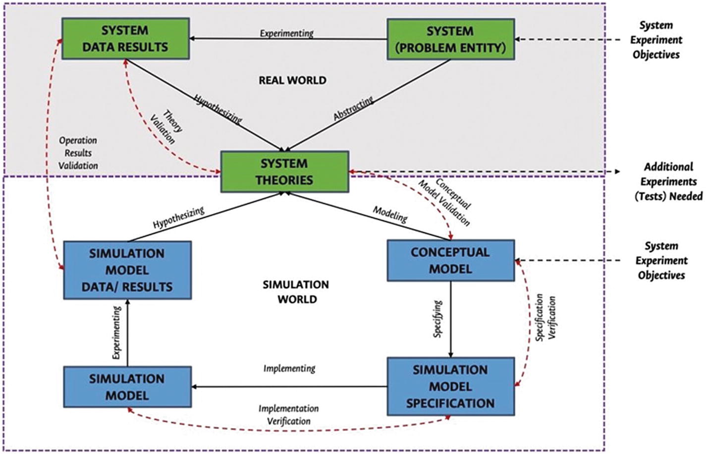
Real world versus simulation world
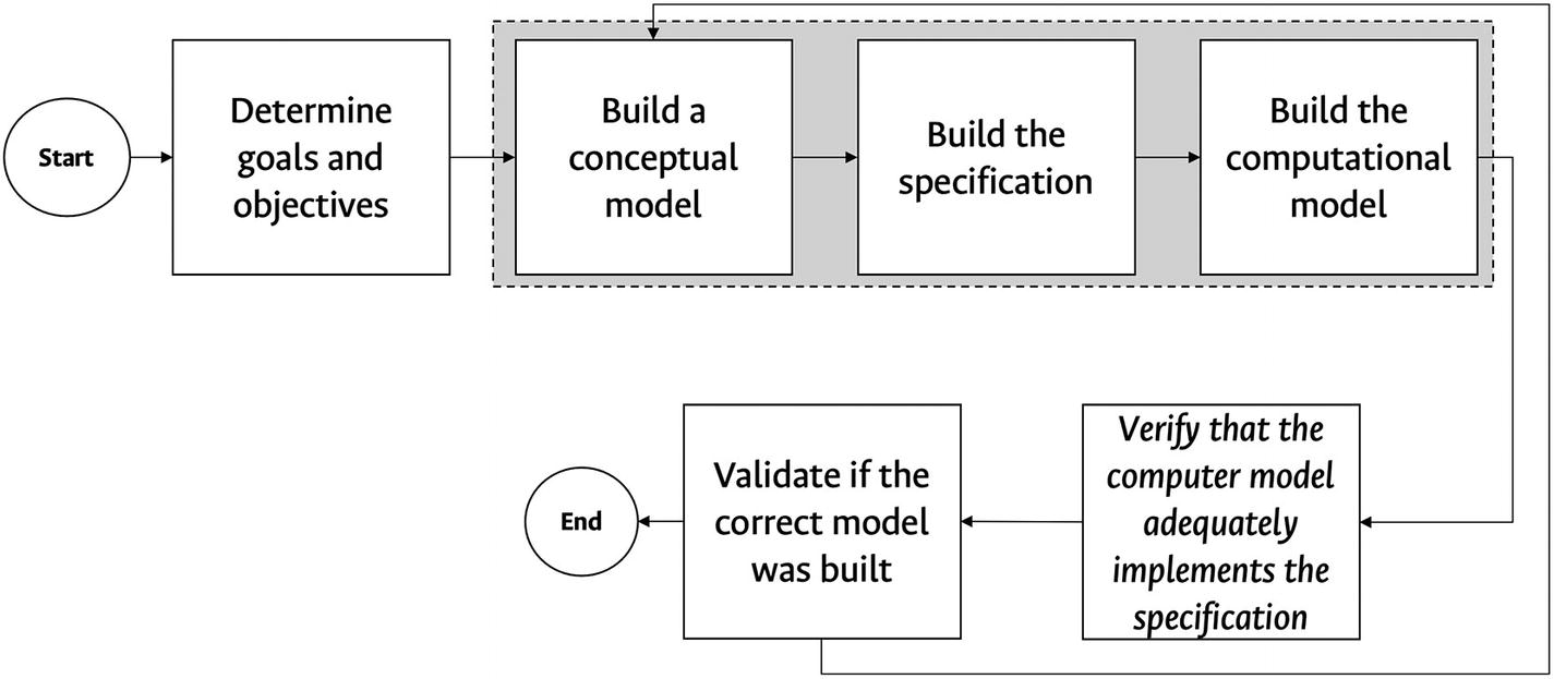
Steps simulation
- 1.Determine goals and objectives.
Boolean decisions: Should another component be added to the model?
Numerical decisions: How many servers in parallel offer optimal performance?
- 2.Build a conceptual model.
What are the important state variables?
How exhaustive should the model be?
- 3.Build the specification.
Collect and statistically analyze data to have “input” models that control the simulation.
In the absence of data, the “input” models should be built using stochastic models that are appropriate for the problem.
- 4.Build the computational model.
Select the language or the simulation tool.
- 5.Verify that the computer model implements the specification properly.
Still not the right model?
- 6.Validate if the correct model was built.
An expert compares the results of the real system with the results of the simulated system.
The system’s animations are useful.
Network Simulators
In communication networks, the development of new routing protocols, algorithms, and architectures is usual. The performance evaluation of these new systems through experimentation can be expensive, the resources may not be available, and valuable features such as scalability are not easy to test in that way. Consequently, simulation becomes an important tool for research since it does not require any physical hardware other than a computer to run the simulations. It provides an economical alternative to evaluate the behavior of these new systems or to test the performance of the existing ones, which under different circumstances are hard to re-create in a laboratory.
Today, it is possible to find different simulation frameworks created by network companies, universities, and academics, whose goal is to offer alternatives, covering different aspects and functionalities of networks. The selection depends on the needs and objectives of the researchers. Besides, it is recommendable to check in bibliographic databases, such as Scopus, for the number of papers that have used a certain simulator and its role on the research.
In Table 1-2, you can see some of the most commonly used network simulations for research. However, keep in mind that there are many networks simulators available, and your selection depends on the objectives of your research and your experience with different programming languages.
ns-3 Simulator General Features
ns-3 is a discrete event network simulator that uses a set of abstractions (node, application, channel, net device, and topology helpers) to simulate devices in communication networks, as well as their services, protocols, and interfaces. The interactions between them are given through multiple channels of communication like Ethernet cables, wireless channels, and power line communication channels, among others.
In a nontechnical explanation, it is possible to define ns-3 as a set of application-oriented telecommunication systems tools with modeling flexibility, with some graphical reporting capabilities and easy-to-use statistical modules.
The development environment is object-oriented through the optional C++ and Python frameworks, with Linux and IOS installers, and includes some useful examples of reusable code and online growth community as support.
Network Simulators
Simulator Framework | License Type |
|---|---|
ns-2 | Open source |
ns-3 | Open source |
Matlab | Commercial |
GlomoSim | Free |
JiST/SWANS | Commercial |
J-Sim | Open source |
OMNeT++ | Open source, academic use licensed |
OPNET | Commercial, free for qualifying universities |
Although it sounds great, you actually need longer periods and patience to run custom simulations. Regardless of your programming skills, based on experience, we recommend working on C++ and Ubuntu Linux LT distributions if possible. In Appendix A, we describe the installation processes of both operating systems.
ns-3 is useful for modeling nonlinear and complex systems, which are impossible to solve from an analytical perspective and often difficult to predict. The typical approach to this obstacle is to reduce complexity by using expert skills to extract conclusions in a reduced ambit and then extend them to other contexts. This feature makes possible the process of formulating well-founded conjectures, which is an important step in a scientific approach.
From our personal experience, we consider that the nature of ns-3 is broader because of its emulation capabilities. One of the main objectives of this simulator is to supply different options to support the emulation and execution of real implementation code. Thus, it allows the opportunity to combine these techniques and reduce experimental discontinuities when moving between simulation, emulation, and real experiments [10].
ns-3 usually runs only one simulation process at a time, which does not limit the scope of possible simulation scenarios. For parallel scenarios, it is required to enable the Message Passing Interface (MPI) and the application program interface (API), which are beyond the scope of this book. In our experience, we tried this with sequential processes, and the results of the repetitive simulation processes were consistent, regardless of the stochastic nature of the data and the real processes modeled. For this reason, it is common to obtain similar results in successive experiments that are desirable from the point of view of accuracy or statistics and acceptable as a simplification of the real world. However, it is possible to add stochastic features to the models. In the following chapters, some examples will be presented and applied specifically to ad hoc networks.
ns-3 has a lot of examples that are useful for new users. Listing 1-1 consists of the topology of two devices (or two nodes) with point-to-point communication of a 5Mbps data rate, a channel, and a delay of 2ms.
ns-3 Example
These two nodes are equipped with a network device that adds a MAC address and a queue to the device. It also has an Internet stack installed that adds IP/TCP/UDP functionality to the existing nodes. A set of IP addresses is then created, and an IPv4 interface is installed on the network device. This interface assigns an IPv4 address to each node on the network device. It then associates this address with the interface and stores it in a container (see Listing 1-2).
ns-3 Example
Then, an application server is created. It waits for UDP packets and then sends them back to the sender, assigning port 9 for this communication. This application created is stored in an application container and assigned to the second node. This application is started at the first second and stopped at second 10 (see Listing 1-3).
ns-3 Example
The next step is to create a client-server application on the first node of the network. It will send UPD packets and wait for a response from the second node. The application has a maximum of 1 packet of 1,024 bytes, and the client will wait 1 second between packets. It will initialize in second 2 of the simulation and stop in second 10 (see Listing 1-4).
ns-3 Example
After defining all the parameters and events of the network, the only thing left is simulating with these four events: one at second 1, one at 2 seconds, and two at 10 seconds (see Listing 1-5).
ns-3 Example
Formal Concepts and ns-3 Specification
In simulators, events are a mandatory abstraction. They can be described in a nonformal definition and, for this book, as a change of state in the model, generally associated with time. Events constitute a causal sequence that allows discovering the evolution of variables as a flow with definite direction. In turn, a discrete event could be explained mathematically through an integer variable. In the simulator, it is common to get two forms of presenting them in the ns-3 screen: as a list of events or as a graphical representation of the behavior of nodes and their interactions, as shown in Figure 1-4. Also, it is possible to output events as trace sinks, Wireshark’s .pcap files, and XML files.
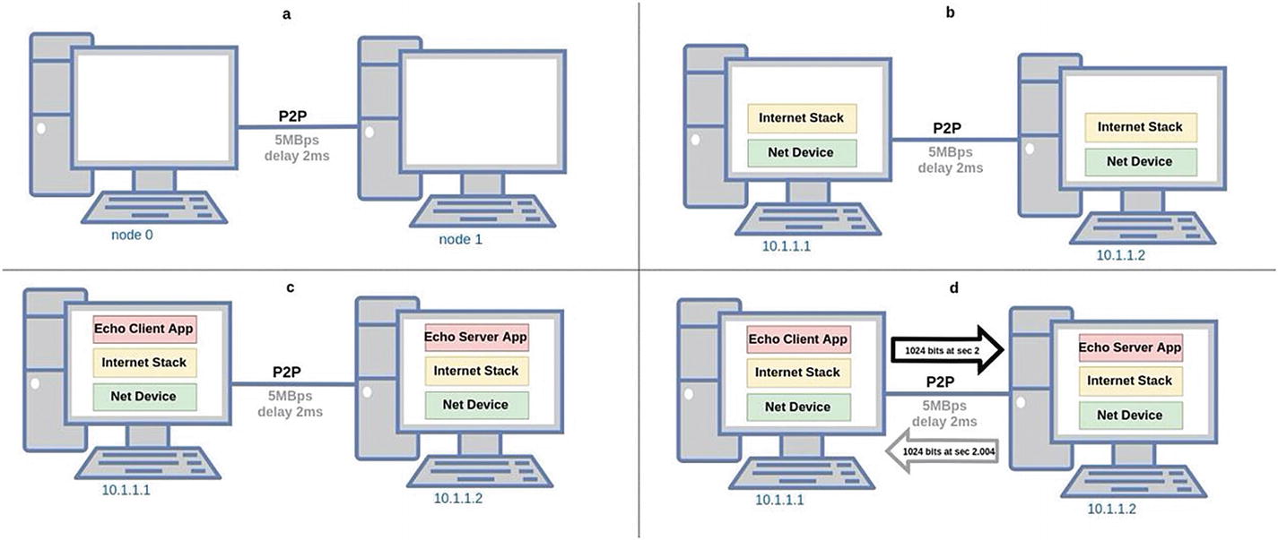
Example 1 of ns-3. a) Creating point-to-point nodes and channels. b) Installing network and Internet stack devices in each node and assigning IP addresses. c) Installing an echo server and client in the nodes. d) Sending a packet and its respective response
Depending on the scope of the simulating job, it is probable that the high-level events presented in Figure 1-4 are the most relevant, especially in a framework of network interaction. Then, in that case, each network event is represented by each screen line. For example, the previous report shows a descriptor of each responsible entity (a network node) that interacts in each previous subprocess. Each node has a network role (server-client) that has its own IPv4 address, a TCP port, and a related primitive service (send-receive).
Here, ns-3 can report some key network events on the screen. However, there are many events (others not shown here) that occur in the background and are associated with the protocols involved. Also, events are associated with the internal programming classes and objects that interact between them. When it is required in .pcap and .xml files, valuable information can be tracked for low-level and detailed interactions and processes.
All of them are discrete events, referred by an arbitrary reference time simulator. It is important to differentiate their time reference from the real-world time reference. The first is an abstract way to order the events; the second one is the conventional user concept and the ones that do not necessarily maintain a clear relationship between them. For example, a user easily understands that on different devices, the executing time is inversely proportional to the performance of the equipment and is associated as a commonsense result. The time reference of the ns-3 event could be independent of the hardware used to build the simulation and even from the released version of the ns-3. For instance, in different devices the third.cc example of simulation delivers the same simulation time result.
According to the previous example, it is possible to appreciate that each event describes an extensively defined frame protocol object and a “nearly” continuous reference time. That suggested by the microsecond-level precision of the time scale reference shown in ns-3 that has an integer as reference time at nanosecond.
When this temporal framework exists, the theoretical approach of the Discrete Event System Specification (DEVS) [11] is used. It is a type of discrete dynamic system with relevant changes occurring at a fixed time. Here, an event is the occurrence of an external trigger or a significant change in an internal variable, often referred to as a model state variable. In ns-3, time advance is managed with a next-event approach. In this technique of discrete event simulation, there is a local program or list of events built as a data structure that updates a timer when the current event occurs. The next or created events are listed in a time-based order until completion [12].
When the simulation time changes asynchronously and discontinuously, the state of the variables is updated “instantly” and remains fixed until the time of the next programmed event changes. In some simulations, this capability can be a comparison metric between experiments. Nevertheless, in the scope of this book, with stochastic variables only, it will be considered as a real-world time framework, always in the context of network traffic, given its burst behavior.
Time is only one element of simulation. In the real world, the interaction between nodes occurs through network interfaces and within nodes through layer interfaces. In the same way, ns-3 represents the same interaction with low-level abstractions represented by the programming objects and entities. For example, a network interface is modeled with a physical or logical port abstraction, identified here by a protocol address. This one-to-one mapping is a system specification formalism called homomorphism , an important approach of ns-3.
As said by Wainer [11], it is feasible to apply modularity with DEVS because it allows an abstract model to be represented, regardless of the simulation techniques used, and to progressively build complex systems. This is another powerful feature of ns-3 associated with its object programming language base. However, this is the reason for decoupling between real-time and event time structure, because object-oriented programming does not have an associated temporal sense.
The default simulated time in ns-3 is not related to the hardware clock; it simply advances to the next event [13]. For the real-time capabilities of ns-3 that are available through the RealTime scheduler, this mode of operation requires an external time source for synchronizing. In this simulated time mode, ns-3 runs in parallel with the external base time between events, while stopping at the event execution (feature currently included ns-3). In this mode, cumulative time differences between the reference and the simulated time may occur, which must be resolved with the configuration options of the RealTime scheduler.
Summary of ns-3 Features
Summary and Classification of Simulator Features | |||
|---|---|---|---|
Feature | Yes | No | Observations |
Discrete event systems | X | – | – |
Parallel discrete events allowed | X | – | – |
Parallel time scripts allowed | X | – | – |
Parallel time events allowed | X | – | – |
Object-oriented programming | – | X | – |
Object-oriented events | X | – | – |
Multicomponent systems interactions allowed | X | – | Individual components system is coupled by connecting their input and output interfaces in a modular way |
Multicomponent events interactions allowed | X | – | Individual events influence all components |
Iterative result | X | – | As defined in customized code |
Input-free systems | X | – | – |
Stochastics generators | X | – | – |
I/O observation frame | X | – | – |
I/O relation observation | X | – | – |
I/O function observation | X | – | – |
I/O system observation | X | – | – |
Block-oriented simulation system | X | – | – |
Chaotic systems allowed | – | X | – |
Noncausal methods | – | X | – |
Fuzzy systems allowed | X | – | – |
Real-time simulating | X | – | – |
Model families allowed | X | – | – |
Error estimating tools | X | – | – |
Graphical model representing | X | – | – |
Graphical experiment representing | X | – | – |
There are other types of modules created by other researches to expand the capabilities of the simulator in fields such as bio-inspired systems [14], [15], artificial intelligence [16], neuronal models [17], among others.
Summary
The ns-3 simulator is based on discrete events to manage the simulation. The simulator has abstractions such as the node, the channel, and the packet. It allows you to create real network models from their abstractions. The simulator allows the simulation and emulation functions to test the models and scenarios on the script. The simulation output can be analyzed as a .pcap file to use another tools such as Wireshark. The ns-3 simulator is a robust tool to design, test, and validate networks, protocols, and architectures on a controlled testbed based on events.
Complementary Readings
Object-oriented modeling and design [18]
Design and analysis of simulation experiments [19]
A gentle introduction to simulation modeling [20]
Yet another network simulator [21]