Tip 53: Selecting Cells Efficiently

Many Excel users think that the only way to select a range of cells is to drag over the cells with the mouse. Although selecting cells with a mouse works, it’s rarely the most efficient way to accomplish the task. A better way is to use your keyboard to select ranges.

Selecting a range by using the Shift and arrow keys

The simplest way to select a range is to press (and hold) Shift and then use the arrow keys to highlight the cells. For larger selections, you can use PgDn or PgUp while pressing Shift to move in larger increments.

You can also use the End key to quickly extend a selection to the last non-empty cell in a row or column. To select the range B3:B8 (see Figure 53-1) by using the keyboard, move the cell pointer to B3 and then press the Shift key while you press End followed by the down-arrow key. Similarly, to select B3:D3, press the Shift key while you press End, followed by the right-arrow key.

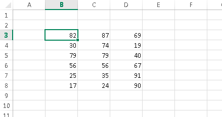
Figure 53-1: A range of cells.

Selecting the current region

Often, you need to select a large rectangular selection of cells — the current region. To select the entire block of cells, move the cell pointer anywhere within the range and press Ctrl+A.

If the cell pointer is within a table (created by using Insert⇒Tables⇒Table), pressing Ctrl+A selects only the data. Press Ctrl+A a second time to select the table’s Header row and Total row.

Selecting a range by Shift+clicking

When you’re selecting a very large range, using the mouse may be the most efficient method — but dragging is not required. Select the upper-left cell in the range. Then scroll to the lower-right corner of the range, press Shift, and click the lower-right cell.

Selecting noncontiguous ranges

Most of the time, your range selections are probably simple rectangular ranges. In some cases, you may need to make a multiple selection — a selection that includes nonadjacent cells or ranges. For example, you may want to apply formatting to cells in different areas of your worksheet. If you make a multiple selection, you can apply the formatting in one step to all selected ranges. Figure 53-2 shows an example of a multiple selection.

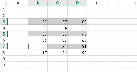
Figure 53-2: A multiple selection that consists of noncontiguous ranges.

You can select a noncontiguous range by using either the mouse or the keyboard.

Press Ctrl as you click and drag the mouse to highlight individual cells or ranges.

From the keyboard, select a range as described previously (by using the Shift key). Then press Shift+F8 to select another range without canceling the previous range selection. Repeat this action as many times as needed. When you’re finished, press Shift+F8 again to return to normal selecting mode.

Selecting entire rows

To select a single row, click a row number along the left of the worksheet. Or select any cell in the row and press Shift+spacebar.

To select multiple adjacent rows, click and drag in the row number area. Or select any cell in the first (or last) row and press Shift+spacebar to select the row. Then press Shift and use the arrow keys to extend the row selection down (or up).

To select multiple nonadjacent rows, press Ctrl while you click the row numbers for the rows you want to include.

Selecting entire columns

To select a single column, click a column letter along the top of the worksheet. Or select any cell in the column and press Ctrl+spacebar.

To select multiple adjacent columns, click and drag in the column letter section. Or select any cell in the first (or last) column and press Ctrl+spacebar to select the column. Then press Shift and use the arrow keys to extend the selection to the right (or left).

To select multiple nonadjacent columns, press Ctrl while you click the column letters for the columns you want to include.

Selecting multisheet ranges

In addition to two-dimensional ranges on a single worksheet, ranges can extend across multiple worksheets to be three-dimensional ranges.

Figure 53-3 shows a simple example of a multisheet workbook. The workbook has four sheets, named Totals, Operations, Marketing, and Manufacturing. The sheets are laid out identically.

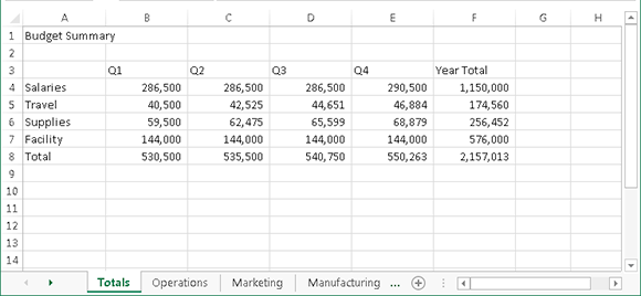
Figure 53-3: Each worksheet in this workbook is laid out identically.

Assume that you want to apply the same formatting to all sheets — for example, you want to make the column headings bold with background shading. Selecting a multisheet range is the best approach. When the ranges are selected, the formatting is applied to all sheets.

In general, selecting a multisheet range is a simple two-step process:

1. Select the range in one sheet.

2. Select the worksheets to include in the range.

To select a group of contiguous worksheets, press Shift and click the sheet tab of the last worksheet that you want to include in the selection. To select individual worksheets, press Ctrl and click the sheet tab of each worksheet that you want to select. When you make the selection, the sheet tabs of the selected sheets appear with a white background, and Excel displays [Group] on the title bar. When you finish working with the multisheet range, click any sheet tab to leave Group mode.

Tip 54: Automatically Filling a Range with a Series

If you need to fill a range with a series of values, one approach is to enter the first value, write a formula to calculate the next value, and copy the formula. For example, Figure 54-1 shows a series of consecutive numbers in column A. Cell A1 contains the value 1, and cell A2 contains this formula, which was copied down the column:

=A1+1

Figure 54-1: Excel offers an easy way to generate a series of values like these.

Another approach is to let Excel do the work by using the handy AutoFill feature:

1. Enter 1 into cell A1.

2. Enter 2 into cell A2.

3. Select A1:A2.

4. Move the mouse cursor to the lower-right corner of cell A2 (the cell’s fill handle), and when the mouse pointer turns into a black plus sign, drag down the column to fill in the cells.

You can turn this behavior on and off. If cells don’t have a fill handle, choose File⇒Options and click the Advanced tab in the Excel Options dialog box. Select the check box labeled Enable Fill Handle and Cell Drag-And-Drop.

The data entered in Steps 1 and 2 provide Excel with the information it needs to determine which type of series to use. If you entered 3 in cell A2, the series will consist of odd integers: 1, 3, 5, 7, and so on.

When you release the mouse button after dragging, Excel displays an Auto Fill Options drop-down list. Click to select other options. The list of options is particular helpful with dates. Figure 54-2 shows the Auto Fill Options when working with a date series. You can quickly create a series of weekdays, months, or years.

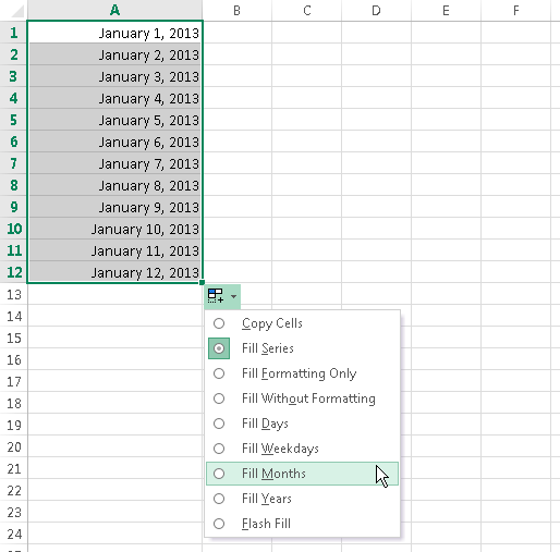
Figure 54-2: Use the Auto Fill Options drop-down list to change the type of fill.

Here’s another AutoFill trick: If the data you start with is irregular, Excel completes the AutoFill action by doing a linear regression and fills in the predicted values. Figure 54-3 shows a worksheet with monthly sales values for January through July. If you use AutoFill after selecting C2:C8, Excel extends the best-fit linear sales trend and fills in the missing values. Figure 54-4 shows the predicted values, along with a chart.

Figure 54-3: Use AutoFill to perform a linear regression and predict sales values for August through December.

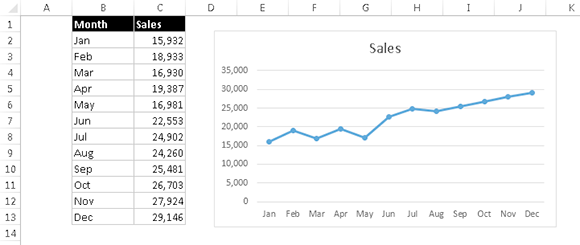
Figure 54-4: The sales figures, after using AutoFill to predict the next five months.

AutoFill also works with dates and even a few text items — day names and month names. The following table lists a few examples of the types of data that can be autofilled.

First Value	Autofilled Values
Sunday	Monday, Tuesday, Wednesday, and so on
Quarter-1	Quarter-2, Quarter-3, Quarter-4, Quarter-1, and so on
Jan	Feb, Mar, Apr, and so on
January	February, March, April, and so on
Month 1	Month 2, Month 3, Month 4, and so on

You can also create your own lists of items to be autofilled. To do so, open the Excel Options dialog box and click the Advanced tab. Then scroll down and click the Edit Custom Lists button to display the Custom Lists dialog box. Enter your items in the List Entries box (each on a new line). Then click the Add button to create the list. Figure 54-5 shows a custom list of region names that use Roman numerals.

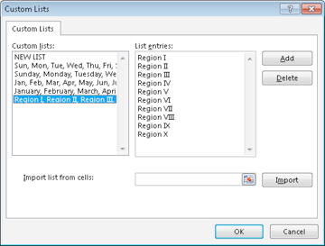
Figure 54-5: These region names work with the Excel AutoFill feature.

Tip 55: Fixing Trailing Minus Signs

Imported data sometimes displays negative values with a trailing minus sign. For example, a negative value may appear as 3,498- rather than the more common -3,498. Excel doesn’t convert these values. In fact, it considers them to be non-numeric text.

The solution is so simple it may surprise you:

1. Select the data that has the trailing minus signs. The selection can also include positive values.

2. Choose Data⇒Data Tools⇒Text to Columns.

3. When the Text to Columns dialog box appears, click Finish.

This procedure works because of a default setting in the Advanced Text Import Settings dialog box (which you don’t even see, normally). To display this dialog box, shown in Figure 55-1, go to Step 3 in the Text to Columns Wizard dialog box and click Advanced.

Or you can use Flash Fill to fix the trailing minus signs. If the range contains any positive values, you may need to provide several examples. See Tip 64 for information about the Flash Fill feature.

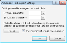
Figure 55-1: The Trailing Minus for Negative Numbers option makes it very easy to fix trailing minus signs in a range of data.

Tip 56: Restricting Cursor Movement to Input Cells

A common type of worksheet uses two types of cells: input cells and formula cells. The user enters data into the input cells, and the formulas calculate and display the results.

Figure 56-1 shows a simple example. The input cells are in the range C4:C7. These cells are used by the formulas in C10:C13. To prevent the user from accidentally typing over formula cells, it’s useful to limit the cursor movement so that the formula cells can’t even be selected.

Figure 56-1: This worksheet has input cells at the top and formula cells below.

Setting up this sort of arrangement is a two-step process: Unlock the input cells and then protect the sheet. The following specific instructions are for the example shown in Figure 56-1:

1. Select C4:C7.

2. Press Ctrl+1 to display the Format Cells dialog box.

3. In the Format Cells dialog box, click the Protection tab, deselect the Locked check box, and click OK.

By default, all cells are locked.

4. Choose Review⇒Changes⇒Protect Sheet.

The Protect Sheet dialog box appears.

5. Deselect the Select Locked Cells check box and make sure that the Select Unlocked Cells check box is selected.

6. (Optional) Specify a password that will be required to unprotect the sheet.

7. Click OK.

After you perform these steps, only the unlocked cells can be selected. If you need to make any changes to your worksheet, you need to unprotect the sheet first, by choosing Review⇒Changes➜Unprotect Sheet.

Although this example used a contiguous range of cells for the input, that isn’t necessary for the steps to work. The input cells can be scattered throughout your worksheet.

Protecting a worksheet with a password isn’t a security feature. This type of password is easily cracked.

Tip 57: Transforming Data with and Without Using Formulas

Often, you have a range of cells containing data that must be transformed in some way. For example, you might want to increase all values by five percent. Or you might need to divide each value by two. This tip describes two ways to perform these types of transformations.

Transforming data without formulas

The following steps assume that you have values in a range and you want to increase all values by five percent. For example, the range can contain a price list and you’re raising all prices by five percent:

1. Activate any empty cell and enter 1.05.

You will multiply the values by this number, which results in an increase of five percent.

2. Press Ctrl+C to copy that cell.

3. Select the range to be transformed.

The range can include values, formulas, or text.

4. Choose Home⇒Clipboard⇒Paste⇒Paste Special to display the Paste Special dialog box (see Figure 57-1).

5. In the Paste Special dialog box, click the Multiply option.

6. Click OK.

7. Press Esc to cancel Copy mode.

Figure 57-1: Using the Paste Special dialog box to multiply a range by a value.

The values in the range are multiplied by the copied value (1.05), and cells that contain text are ignored. Formulas in the range are modified accordingly. Assume that the range originally contained this formula:

=SUM(B18:B22)

After you perform the Paste Special operation, the formula is converted to

=(SUM(B18:B22))*1.05

This technique is limited to the four basic math operations: add, subtract, multiply, and divide.

For more versatility, keep reading to learn how to use formulas to transform values.

Transforming data by using temporary formulas

The previous section describes how to perform simple mathematical transformations on a range of numeric data. This tip describes the much more versatile method of transforming data (numerical or text) by using temporary formulas.

Figure 57-2 shows a worksheet with names in column A. These names are in all uppercase letters, and the goal is to convert them to proper case (only the first letter of each name is uppercase).

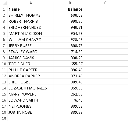
Figure 57-2: The goal is to transform the names in column A to proper case.

Follow these steps to transform the data in column A:

1. Create a temporary formula in an unused column.

For this example, enter this formula in cell C2:

=PROPER(A2)

2. Copy the formula down the column to accommodate all cells to be transformed.

3. Select the formula cells (in column C).

4. Press Ctrl+C.

5. Select the original data cells (in column A).

6. Choose Home⇒Clipboard⇒Paste⇒Paste Values (V).

The original data is replaced with the transformed data (see Figure 57-3).

7. Press Esc to cancel Copy mode.

8. When you’re satisfied that the transformation happened as you intended, you can delete the temporary formulas in column C.

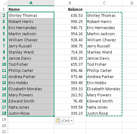
Figure 57-3: The formula results from column C replace the original data in column A.

You can adapt this technique for just about any type of data transformation you need. The key, of course, is constructing the proper transformation formula in Step 1.

Tip 58: Creating a Drop-Down List in a Cell

Most Excel users probably assume that some advanced feature (such as a VBA macro) is required to display a drop-down list in a cell. But it’s not. You can easily display a drop-down list in a cell — no macros required.

Figure 58-1 shows an example. Cell B2, when selected, displays a down arrow. Click the arrow, and you get a list of items (in this case, month names). Click an item, and it appears in the cell. The drop-down list can contain text, numeric values, or dates. Your formulas, of course, can refer to cells that contain a drop-down list. The formulas always use the value that’s currently displayed.

Figure 58-1: Creating a drop-down list in a cell is easy and doesn’t require macros.

The trick to setting up a drop-down list is to use the data validation feature. The following steps describe how to create a drop-down list of items in a cell:

1. Enter the list of items in a range.

In this example, the month names are in the range F1:F12.

2. Select the cell that will contain the drop-down list (cell B2, in this example).

3. Choose Data⇒Data Tools⇒Data Validation.

4. In the Data Validation dialog box, click the Settings tab.

5. In the Allow drop-down list, select List.

6. In the Source box, specify the range that contains the items.

In this example, the range is E1:E12.

7. Make sure that the In-Cell Dropdown option is checked (see Figure 58-2) and click OK.

If your list is short, you can avoid Step 1. Rather, just type your list items (separated by commas) in the Source box in the Data Validation dialog box.

If you plan to share your workbook with others who use Excel 2007 or earlier, make sure that the list is on the same sheet as the drop-down list. Alternatively, you can put the list on any sheet, as long as it’s a named range. For example, you can choose Formulas⇒Defined Names⇒Define Name to define the name MonthNames for E1:E12. Then, in the Data Validation dialog box, enter =MonthNames in the Source box.

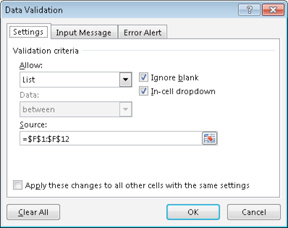
Figure 58-2: Using the Data Validation dialog box to create a drop-down list.

Tip 59: Comparing Two Ranges by Using Conditional Formatting

A common task is comparing two lists of items to identify differences between the two lists. Doing it manually is far too tedious and error-prone, but Excel can make it easy. This tip describes a method that uses conditional formatting.

Figure 59-1 shows an example of two multicolumn lists of names. Applying conditional formatting can make the differences in the lists become immediately apparent. These list examples contain text, but this technique also works with numeric data.

Figure 59-1: You can use conditional formatting to highlight the differences in these two ranges.

The first list is in A2:A20, and this range is named OldList. The second list is in C2:C20, and the range is named NewList. The ranges were named by using the Formulas⇒Defined Names⇒Define Name command. Naming the ranges isn’t necessary, but it makes them easier to work with.

Start by adding conditional formatting to the old list:

1. Select the cells in the OldList range.

2. Choose Home⇒Conditional Formatting⇒New Rule to display the New Formatting Rule dialog box.

3. In the New Formatting Rule dialog box, click the option labeled Use a Formula to Determine Which Cells to Format.

4. Enter this formula in the dialog box (see Figure 59-2):

=COUNTIF(NewList,A2)=0

When using this technique with your own data, substitute the actual range address (or name) for NewList, and substitute the address of the top left selected cell for A2.

5. Click the Format button and specify the formatting to apply when the condition is true.

A different fill color is a good choice.

6. Click OK.

Figure 59-2: Applying conditional formatting.

The cells in the NewList range use a similar conditional formatting formula.

1. Select the cells in the NewList range.

2. Choose Home⇒Conditional Formatting⇒New Rule to display the New Formatting Rule dialog box.

3. In the New Formatting Rule dialog box, click the option labeled Use a Formula to Determine Which Cells to Format.

4. Enter this formula in the dialog box:

=COUNTIF(OldList,C2)=0

When using this technique with your own data, substitute the actual range address (or name) for OldList, and substitute the address of the top left selected cell for C2.

5. Click the Format button and specify the formatting to apply when the condition is true (a different fill color).

6. Click OK.

Figure 59-3 shows the result. Names that are in the old list but not in the new list are highlighted. In addition, names in the new list that aren’t in the old list are highlighted in a different color. Names that aren’t highlighted appear in both lists.

Figure 59-3: Conditional formatting causes differences in the two lists to be highlighted.

Both of these conditional-formatting formulas use the COUNTIF function. This function counts the number of times a particular value appears in a range. If the formula returns 0, it means that the item doesn’t appear in the range. Therefore, the conditional formatting kicks in and the cell’s background color is changed.

Tip 60: Finding Duplicates by Using Conditional Formatting

You might find it helpful to identify duplicate values within a range of cells. For example, take a look at Figure 60-1. Are any of the values duplicated?

One approach to identifying duplicate values is to use conditional formatting. After applying a conditional formatting rule, you can quickly spot duplicated cell values.

Figure 60-1: You can use conditional formatting to quickly identify duplicate values in a range.

Here’s how to set up the conditional formatting:

1. Select the cells in the range (in this example, A1:G22).

2. Choose Home⇒Conditional Formatting⇒New Rule to display the Conditional Formatting dialog box.

3. In the Conditional Formatting dialog box, select the option labeled Use a Formula to Determine Which Cells to Format.

4. For this example, enter this formula (change the range references to correspond to your own data):

=COUNTIF($A$1:$G$22,A1)>1

5. Click the Format button and specify the formatting to apply when the condition is true.

Changing the fill color is a good choice.

6. Click OK.

Figure 60-2 shows the result. The seven highlighted cells are the duplicated values in the range.

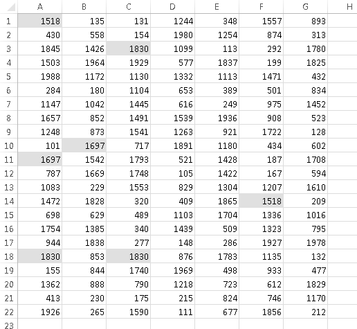
Figure 60-2: Conditional formatting causes the duplicated cells to be highlighted.

You can extend this technique to identify entire rows within a list that are identical. The trick is to add a new column and use a formula that concatenates the data in each row. For example, if your list is in A2:G500, enter this formula in cell H2:

=A2&B2&C2&D2&E2&F2&G2

Copy the formula down the column and then apply the conditional formatting to the formulas in column H. In this case, the conditional formatting formula is

=COUNTIF($H$2:$H$500,H2)>1

Highlighted cells in column H indicate duplicated rows.

You can use Data⇒Data Tools⇒Remove Duplicates to remove duplicate rows. That command, however, doesn’t identify the duplicates before deleting them.

Tip 61: Working with Credit Card Numbers

If you’ve ever tried to enter a 16-digit credit card number into a cell, you may have discovered that Excel always changes the last digit to a zero. Even worse, maybe you didn’t discover the changed credit card number until it was too late.

Why does Excel change your numbers? The reason is that Excel can handle only 15 digits of numerical accuracy.

Entering credit card numbers manually

If you need to store credit card numbers in a worksheet, you have three options:

→ Precede the credit card number with an apostrophe. Excel then interprets the data as a text string rather than as a number.

→ Preformat the cell or range by using the Text number format. Select the range, choose Home⇒Number and then select Text from the Number Format drop-down control.

→ Enter the card number with dashes or spaces. Embedding a dash character (or any other non-numeric character) forces Excel to interpret the entry as text.

This tip, of course, also applies to other long numbers (such as part numbers) that aren’t used in numeric calculations.

Importing credit card numbers

If you’re importing credit card numbers from a CSV text file, Excel will import the credit card numbers as values — and erroneously change the last digit to zero. To avoid this, don’t use File⇒Open to import the text. Rather, use Data⇒Connections⇒Get External Data⇒From Text. When you use this command, Excel displays the TextImport Wizard. In Step 3 of the wizard, make sure that you specify Text as the column data format for the credit card numbers. See Figure 61-1.

Figure 61-1: Using the TextImport Wizard to ensure that credit card numbers are imported as text.

Tip 62: Identifying Excess Spaces

A common type of spreadsheet error involves something that you can’t even see: a space character. Consider the example shown in Figure 62-1. Cell B2 contains a formula that looks up the color name in cell B1 and returns the corresponding code from a table. The formula is

=VLOOKUP(B1,D2:E9,2,FALSE)

Figure 62-1: A simple lookup formula returns the code for a color entered in cell B1.

In Figure 62-2, the formula in cell B2 returns an error — indicating that Red wasn’t found in the table. Hundreds of thousands of Excel users have spent far too much time trying to figure out why this sort of thing doesn’t work. In this case, the answer is simple: Cell D7 doesn’t contain the word Red. Rather, it contains the word Red followed by a space. To Excel, these text strings are completely different.

Figure 62-2: The lookup formula can’t find the word Red in the table.

If your worksheet contains thousands of text entries — and you need to perform comparisons using that text — you may want to identify the cells that contain excess spaces and then fix those cells. The term excess spaces means a text entry that contains any of the following:

→ One or more leading spaces

→ One or more trailing spaces

→ Two or more consecutive spaces within the text

One way to identify this type of cell is to use conditional formatting. To set up conditional formatting to identify excess spaces, follow these steps:

1. Select all text cells to which you want to apply conditional formatting.

2. Choose Home⇒Conditional Formatting⇒New Rule to display the New Formatting Rule dialog box.

3. In the top part of the dialog box, select the option labeled Use a Formula to Determine Which Cells to Format.

4. Enter a formula like the following in the bottom part of the dialog box (see Figure 62-3):

=A1<>TRIM(A1)

Note: This formula assumes that cell A1 is the upper-left cell in the selection. If that’s not the case, substitute the address of the upper-left cell in the selection you made in Step 1.

5. Click the Format button to display the Format Cells dialog box and select the type of formatting you want for the cells that contain excess spaces — for example, a yellow fill color.

6. Click OK to close the Format Cells dialog box, and click OK again to close the New Formatting Rule dialog box.

After you complete these steps, each cell that contains excess spaces and is within the range you selected in Step 1 is highlighted with the formatting of your choice. You can then easily spot these cells and remove the spaces.

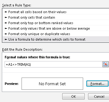
Figure 62-3: Using conditional formatting to identify cells that contain excess spaces.

Because of the way the TRIM function works, the formula in Step 4 also applies the conditional formatting to all numeric cells. A slightly more complex formula that doesn’t apply the formatting to numeric cells is

=IF(NOT(ISNONTEXT(A1)),A1<>TRIM(A1))

Tip 63: Transposing a Range

You may have a range of data that should be transposed. Transposing a range is essentially making the rows columns, and the columns rows. Figure 63-1 shows an example. The original data is in A1:H9, and the transposed data is in A12:I19.

This tip describes two methods to transpose a range of data.

Figure 63-1: Data before and after being transposed.

Using Paste Special

To transpose a range of data by copying and pasting, follow these steps:

1. Select the range to be transposed.

2. Press Ctrl+C to copy the range.

3. Select the cell that will be the upper-left cell for the transposed range.

4. Choose Home⇒Clipboard⇒Paste⇒Paste Special to display the Paste Special dialog box.

5. Choose the Transpose option.

6. Click OK.

Excel pastes the copied data, but reoriented.

If the original range contains formulas, the formulas will be adjusted so they continue to refer to the correct cells.

If the original range is in a table (created with Insert⇒Tables⇒Table), this technique has a few caveats. The original selection cannot include the Total Row or columns that contain a formula. You can still paste the transposed data, but you must choose the Values option in the Paste Special dialog box. The transposed range will include the values (but not the formulas).

Using the TRANSPOSE function

In some cases, you may want the transposed range to be linked to the original range. In such a situation, changes made to the original range also appear in the transposed range. Here’s how to set up a transposed range that’s linked to the original source. Refer to Figure 63-2.

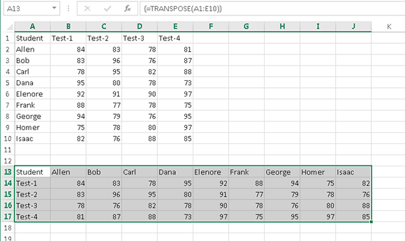
Figure 63-2: A13:J17 contains a multicell array formula, linked to the source range.

1. Make a note of the number of rows and columns in the source range.

In this example, the source range (A1:E10) has 10 rows and 5 columns.

2. Select a range of blank cells that has the same number of rows as source range columns, and the same number of column as source range rows.

In this example, the selection should be 5 rows and 10 columns. For example, you can put the transposed range in A13:J17.

3. Type a formula that uses the TRANSPOSE function, with the source range address as its argument.

In this example, the formula is

=TRANSPOSE(A1:E10)

4. Press Ctrl+Shift+Enter (not just Enter) to create a multicell array formula in all of the selected cells.

Any changes made in the source range also appear in the transposed range.

Tip 64: Using Flash Fill to Extract Data

When you import data, it’s often necessary to clean up some of the text. For example, names may appear in uppercase that they should be in proper case. One approach is to use formulas to modify the text (see Tip 57). Another approach uses a feature introduced in Excel 2013: Flash Fill.

Flash Fill uses pattern recognition to extract data (and also concatenate data) from adjoining columns. Just enter a few examples in a column that’s adjacent to the data, and then choose Data⇒Data Tools⇒Flash Fill (or press Ctrl+E). Excel analyzes the examples you typed and attempts to fill in the remaining cells. If Excel didn’t recognize the pattern you had in mind, press Ctrl+Z, add another example or two, and try again.

Changing the case of text

Figure 64-1 shows a list of U.S. presidents in column A. Column B shows the result of using Flash Fill to convert the text to proper case.

Start by providing a few examples: Type George Washington in cell B1 and John Adams in cell B2. You’ll notice that Excel kicks in as soon as you start typing John Adams. It recognizes your pattern (which is “make all text proper case”) and fills the column with the transformed text (in a light gray color). You can press Enter to keep Excel’s suggestion, or continue typing more examples. At any time, you can press Ctrl+E to have Excel fill the column.

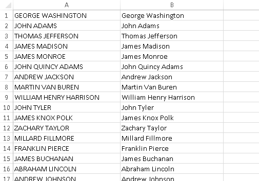
Figure 64-1: Flash Fill quickly converted the names in Column A to proper case.

Extracting last names

In this example, we want to extract the last name of each president, so the list can be sorted by last name. This is a simple job for Flash Fill. It takes only two examples, and the pattern is recognized.

Figure 64-2 shows the worksheet after Excel extracted the last names. Now, you can sort the list by column C, so the name will be in alphabetical order, by last name.

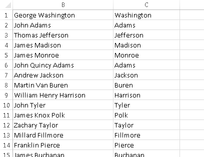
Figure 64-2: Flash Fill extracted the last names.

Extracting first names

You’ll find that Flash Fill is equally adept at extracting first names. Figure 64-3 shows the list of presidents after using Flash Fill to extract the first names in Column D. Again, it took only two examples before Excel identified the pattern.

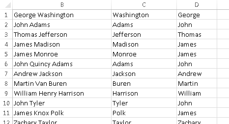
Figure 64-3: Flash Fill extracted the first names.

Extracting middle names

Some (but not all) of the presidents on the list have a middle name. Can Flash Fill extract the middle names?

The answer: Sort of. I provided several examples of middle names, and Flash Fill successfully extracted the other middle names. But for names without a middle name, it extracted the first name. No matter what I tried, I could not get Flash Fill to ignore names that had no middle name.

Extracting domain names from URLs

Here’s another example of using Flash Fill. Say you have a list of URLs and need to extract the filename (the text that follows the last slash character).

Figure 64-4 shows a list of URLs. Flash Fill required just one example of a filename entered in column B. I pressed Ctrl+E, and Excel filled in the remaining rows. Flash fill worked equally well removing the filename from the URL, in column C.

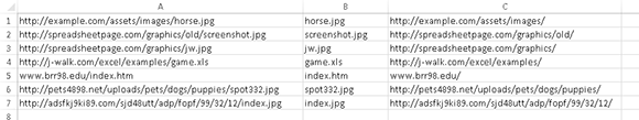
Figure 64-4: Flash Fill extracted the filenames from URLs.

Potential problems

Flash Fill is a great feature, but if you use it for important data, you should be aware of some potential problems:

→ Sometimes it just doesn’t work. Extracting middle names seems like a simple pattern, but Flash Fill was not capable of recognizing the pattern.

→ It’s not always accurate. With a small set of data, it’s usually easy to check to ensure that Flash Fill worked as you intended it to work. But if you use Flash Fill on thousands of rows of data, you can’t be assured that it worked perfectly unless you examine every row. Flash Fill works best with data that is very consistent.

→ It’s not dynamic. If you change any of the information that Flash Fill used, the changes are not reflected in the filled column.

→ There is no “audit trail.” If you use formulas to extract data, the formulas provide documentation so anyone can figure out how the data was extracted. Using Flash Fill, on the other hand, provides no such audit trail. There is no way to see which rules Excel used to extract the data.

Tip 65: Using Flash Fill to Combine Data

Tip 64 described how to extract data using the Excel 2013 Flash Fill feature. This tip looks at the other side of Flash Fill: combing data.

If you need to combine the data in two or more columns, you can write a formula that uses the concatenation operator (&). For example, this formula combines the contents of cells A1, B1, and C1:

=A1&B1&C1

For more complicated types of combinations, Flash Fill might be able to do the job and save you the trouble of creating (and debugging) a formula.

Figure 65-1 shows a worksheet with first names in column A and last names in column B. I used Flash Fill to create e-mail addresses (in Column C) for the domain example.com. The e-mail addresses consist of the first initial, an underscore, and the last name — all lowercase.

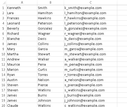
Figure 65-1: Flash Fill can quickly convert these names into e-mail addresses.

It took only two examples before Flash Fill recognized the pattern and filled in the rest of the column.

Flash Fill is simpler than composing this equivalent formula:

=LOWER(LEFT(A1,1)&”_”&B1&”@example.com”)

Figure 65-2 shows another example. Column A:D hold the original data, and the text in column E was filled in using Flash Fill, after providing two examples. The equivalent formula to generate the text in column E is

=A4&” “&B4&”: “&TEXT(D4,”$0”)&” due on 10/”&C4&”/2013”

Figure 65-2: Flash Fill generated the text in column E.

Tip 66: Inserting Stock Information

This tip describes how to insert refreshable stock data into a worksheet. For some reason, Microsoft makes this feature rather difficult to find.

Here’s how to do it:

1. Make sure that you’re connected to the Internet.

2. Type a stock symbol into a cell — for example, MSFT for Microsoft. Make sure the characters are all uppercase.

3. Right-click the cell and choose Addition Cell Actions⇒Insert Refreshable Stock Price from the shortcut menu.

The Insert Stock Price dialog box appears.

4. Specify the location for the information (on a new sheet, or starting at a particular cell).

5. Click OK.

Excel retrieves current information about the stock and inserts data that occupies 18 rows and 16 columns (see Figure 66-1).

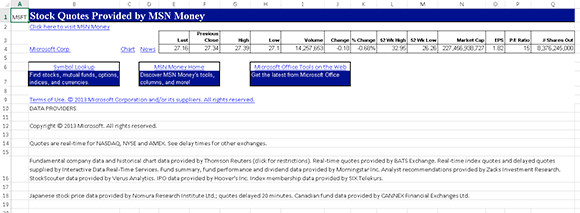
Figure 66-1: Refreshable stock information inserted into a worksheet.

You can refresh the information at any time. Select any cell in the table, right-click, and choose Refresh from the shortcut menu. If your worksheet has information for multiple stocks, you can refresh them all by choosing Data⇒Connections⇒Refresh All.

Hiding irrelevant rows and columns

Notice that, of the 18 rows, only one of them contains actual data. The other rows are links and disclaimers. Unfortunately, there is no direct way to retrieve the information without all of the extraneous information. But you can hide the irrelevant rows and columns — and the hidden rows and columns remain hidden when you refresh the information.

Figure 66-2 shows a worksheet that has information for four stocks. I hid the irrelevant rows and columns, for a concise display.

Figure 66-2: Information for four stocks, after hiding irrelevant rows and columns.

Behind the scenes

Using the Addition Cell Actions⇒Insert Refreshable Stock Price shortcut menu item is just a quick way of performing a web query and retrieving data from Microsoft’s MSN Money site. You can retrieve the same information by performing a web query. Choose Data⇒Get External Data⇒From Web and use this URL:

http://moneycentral.msn.com/investor/external/excel/quotes.asp?symbol=MSFT

The URL retrieves information for Microsoft. You can replace MSFT with a different stock symbol. Figure 66-3 shows the New Web Query dialog box before the information is inserted into a worksheet.

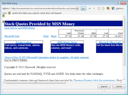
Figure 66-3: Using the New Web Query dialog box to retrieve stock information.

  See Tip 67 for more information about web queries.

Tip 67: Getting Data from a Web Page

This tip describes three ways to capture data contained on a web page:

→ Paste a static copy of the information.

→ Create a refreshable link to the site.

→ Open the page directly in Excel.

Pasting static information

One way to get data from a web page into a worksheet is to simply highlight the text in your browser, press Ctrl+C to copy it to the Clipboard, and then paste it into a worksheet. The results will vary, depending on what browser you use and how the web page is coded.

If pasting doesn’t yield the results you want, choose Home⇒Clipboard⇒Paste⇒Paste Special and then try various paste options.

Figure 67-1 shows some currency exchange rates, pasted from a web page at msn.com. As you can see, even the hyperlinks are pasted.

Figure 67-1: A table of exchange rates copied from a website and pasted to a worksheet.

Pasting refreshable information

If you need to regularly access updated data from a web page, create a web query. Figure 67-1 shows a website that contains currency exchange rates in a three-column table.

The term web query is a bit misleading because this operation is not limited to the web. You can perform a web query on a local HTML file, a file stored on a network server, or a file stored on a web server on the Internet. To retrieve information from a web server, you must be connected to the Internet. After the information is retrieved, an Internet connection is not required to work with the information (unless you need to refresh the query).

These steps create a web query that allows this information to be retrieved and then refreshed at any time with a single mouse click:

1. Choose Data⇒Get External Data⇒From Web to display the New Web Query dialog box.

2. In the Address field, enter the URL of the website and click Go.

For this example, the URL for the web page shown in Figure 67-2 is

http://investing.money.msn.com/investments/exchange-rates

Notice that the New Web Query dialog box contains a web browser (Internet Explorer). You can click links and navigate the website until you locate the data you’re interested in.

When a web page is displayed in the New Web Query dialog box, you see one or more yellow boxes with an arrow, which correspond to tables defined in the web page — plus another yellow box that will retrieve the entire page.

3. Click a yellow box, and it turns into a green check box, which indicates that the data in that table will be imported.

Unfortunately, the table in the example is not selectable, so the only choice is to retrieve the entire page.

4. Click the Import button to display the Import Data dialog box.

5. In the Import Data dialog box, specify the location for the imported data.

It can be a cell in an existing worksheet or a new worksheet.

6. Click OK, and Excel imports the data.

Figure 67-2: Using the New Web Query dialog box to specify the data to be imported.

Part of the results is shown in Figure 67-3. Although I was interested only in the 17-row and 3-column currency table, this web query retrieved 145 rows of mostly irrelevant information.

By default, the imported data is a web query. To refresh the information, right-click any cell in the imported range and choose Refresh from the shortcut menu.

If you don’t want to create a refreshable query, specify this choice in Step 5 of the preceding step list. In the Import Data dialog box, click the Properties button and deselect the Save Query Definition check box.

Excel’s Web query feature works by identifying tables (specified using the HTML <TABLE> tag) in the document. Increasingly, website designers use cascading style sheets (CSS) to display tabular information. As demonstrated in this example, Excel doesn’t recognize these as tables and, therefore, doesn’t display a yellow arrow so you can retrieve only the table. Therefore, you may have to retrieve the entire document and then delete (or hide) everything except the table that you want.

Figure 67-3: Information retrieved from a web query.

Opening the web page directly

Another way to get web page data into a worksheet is to open the URL directly, by using Excel’s File⇒Open command. Just enter the complete URL into the File Name field and click Open.

The results will vary, depending on how the web page is laid out. Most of the time, you’ll get satisfactory results. In some cases, you’ll retrieve quite a bit of extraneous information. Also, note that the information is not refreshable. If the data on the web page changes, you’ll need to close the workbook and use the File⇒Open command again.

Tip 68: Importing a Text File into a Worksheet Range

If you need to insert a text file into a specific range in a worksheet, you may think that your only choice is to import the text into a new workbook (by choosing Office⇒Open) and then to copy the data and paste it to the range where you want it to appear. However, you can do it in a more direct way.

Figure 68-1 shows a small CSV (comma separated value) file. The following instructions describe how to import this file, named monthly.csv, beginning at cell C3.

Figure 68-1: This CSV file will be imported into a range.

1. Choose Data⇒Get External Data⇒From Text to display the Import Text File dialog box.

2. Navigate to the folder that contains the text file.

3. Select the file from the list and then click the Import button to display the Text Import Wizard.

4. Use the Text Import Wizard to specify how the data will be imported.

For a CSV file, specify Delimited, with a Comma Delimiter.

5. Click the Finish button.

The Import Data dialog box appears.

6. Click the Properties button, and the External Data Range Properties dialog box appears.

7. Deselect the Save Query Definition check box and click OK to return to the Import Data dialog box.

8. Here, specify the location for the imported data.

It can be a cell in an existing worksheet or a new worksheet.

9. Click OK, and Excel imports the data (see Figure 68-2).

You can ignore Step 7 if the data you’re importing will be changing. By saving the query definition, you can quickly update the imported data by right-clicking any cell in the range and choosing Refresh.

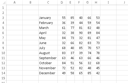
Figure 68-2: This range contains data imported directly from a CSV file.

Tip 69: Using the Quick Analysis Feature

One of the new features in Excel 2013 is Quick Analysis. When you select a range of data, Excel displays a Quick Analysis button in the lower-right corner of the range. Click the button to view some options, shown in Figure 69-1. You can also press Ctrl+Q on the keyboard to display the Quick Analysis options.

Figure 69-1: Quick Analysis options for the selected range.

The words along the top (Formatting, Charts, Totals, Tables, and Sparklines) are menu items. Click an item and a different set of icons appears. When you hover your mouse over an icon, Excel sometimes displays a preview of how the option will appear.

The options available depend on the type of data in the selected range. For example, if the range contains only text, the Sparklines option will not be available.

Figure 69-2 shows an example of a range of numbers in column C, with a preview of the Quick Analysis option to create running totals in column D.

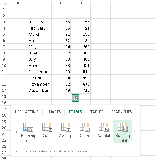
Figure 69-2: A preview of Quick Analysis running totals.

Figure 69-3 shows another example. The range A2:G7 is selected, and Quick Analysis is previewing the Line Sparklines option in column H.

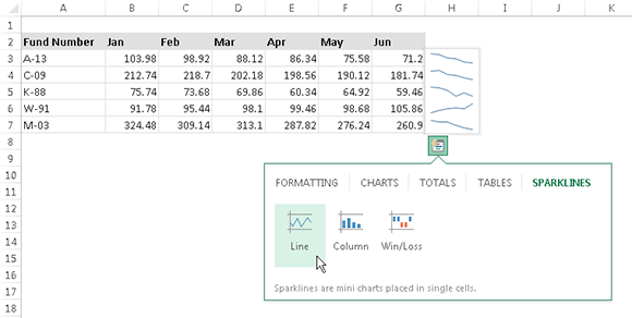
Figure 69-3: A preview of Quick Analysis Sparklines.

The Quick Analysis options don’t enable you to do anything that you can’t do using Excel’s normal commands. But sometimes it can you save a bit of time. If you find the Quick Analysis button annoying, turn if off in the General tab of the Excel Options dialog box. Deselect the check box labeled Show Quick Analysis Options on Selection.

Tip 70: Filling the Gaps in a Report

When you import data, you can sometimes end up with a worksheet that looks something like the one shown in Figure 70-1. This type of report formatting is common. As you can see, an entry in column A applies to several rows of data. If you sort this type of list, the missing data messes things up, and you can no longer tell who sold what when.

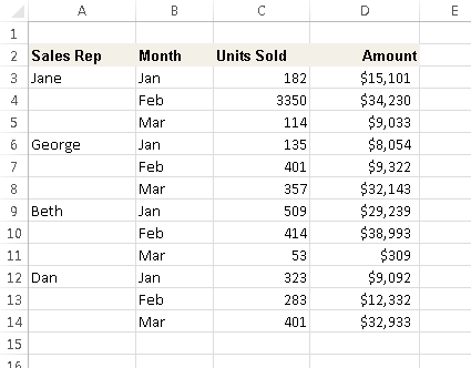
Figure 70-1: This report contains gaps in the Sales Rep column.

If your list is small, you can enter the missing cell values manually or by using a series of Home➜Editing⇒Fill⇒Down commands (or its Ctrl+D shortcut). But if you have a large list that’s in this format, you need a better way of filling in those cell values. Here’s how:

1. Select the range that has the gaps (A3:A14, in this example).

2. Choose Home⇒Editing⇒Find & Select⇒Go To Special.

The Go To Special dialog box appears.

3. Select the Blanks option and click OK.

This action selects the blank cells in the original selection.

4. On the Formula bar, type an equal sign (=) followed by the address of the first cell with an entry in the column (=A3, in this example) and press Ctrl+Enter.

5. Reselect the original range and press Ctrl+C to copy the selection.

6. Choose Home⇒Clipboard⇒Paste⇒Paste Values to convert the formulas to values.

After you complete these steps, the gaps are filled in with the correct information, and your worksheet looks similar to the one shown in Figure 70-2. Now it’s a normal list, and you can do whatever you like with it — including sorting.

Figure 70-2: The gaps are gone, and this list can now be sorted.

Tip 71: Performing Inexact Searches

If you have a large worksheet with lots of data, locating what you’re looking for can be difficult. The Excel Find and Replace dialog box is a useful tool for locating information, and it has a few features that many users overlook.

Access the Find and Replace dialog box by choosing Home⇒Editing⇒Find & Select⇒Find (or by pressing Ctrl+F). If you’re replacing information, you can use Home⇒Editing⇒Find & Select⇒Replace (or Ctrl+H). The only difference is which of the two tabs is displayed in the dialog box. Figure 71-1 shows the Find and Replace dialog box after clicking the Options button, which expands the dialog box to show additional options.

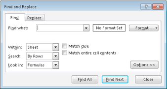
Figure 71-1: The Find and Replace dialog box with the Find tab selected.

In many cases, you want to locate “approximate” text. For example, you may be trying to find data for a customer named Stephen R. Rosencrantz. You can, of course, search for the exact text: Stephen R. Rosencrantz. However, there’s a reasonably good chance that the search will fail. The name may have been entered differently, as Steve Rosencrantz or S.R. Rosencrantz, for example. It may have even been misspelled as Rosentcrantz.

The most efficient search for this name is to use a wildcard character and search for st*rosen* and then click the Find All button. In addition to reducing the amount of text that you enter, this search is practically guaranteed to locate the customer, if the record is in your worksheet. The search may also find some records that you aren’t looking for, but that’s better than not finding anything.

The Find and Replace dialog box supports two wildcard characters:

→ ? matches any single character.

→ * matches any number of characters.

Wildcard characters also work with values. For example, searching for 3* locates all cells that contain an entry that begins with 3. Searching for 1?9 locates all three-digit entries that begin with 1 and end with 9.

To search for a question mark or an asterisk, precede the character with a tilde character (~). For example, the following search string finds the text *NONE*:

~*NONE~*

If you need to search for the tilde character, use two tildes.

If your searches don’t seem to be working correctly, double-check these three options (which sometimes have a way of changing on their own):

→ Match Case: If this check box is selected, the case of the text must match exactly. For example, searching for smith does not locate Smith.

→ Match Entire Cell Contents: If this check box is selected, a match occurs if the cell contains only the search string (and nothing else). For example, searching for Excel doesn’t locate a cell that contains Microsoft Excel.

→ Look In: This drop-down list has three options: Values, Formulas, and Comments. If, for example, Values is selected, searching for 900 doesn’t find a cell that contains 900 if that value is generated by a formula.

Remember that searching operates on the selected range of cells. If you want to search the entire worksheet, select only one cell before you begin your search.

Also, remember that searches do not include numeric formatting. For example, if you have a value that uses currency formatting so that it appears as $54.00, searching for $5* doesn’t locate that value.

Working with dates can be a bit tricky because Excel offers many ways to format dates. If you search for a date by using the default date format, Excel locates the dates even if they’re formatted differently. For example, if your system uses the m/d/y date format, the search string 10/*/2013 finds all dates in October 2013, regardless of how the dates are formatted.

You can also use an empty Replace With field. For example, to quickly delete all asterisks from your worksheet, enter ~* in the Find What field and leave the Replace With field blank. When you click the Replace All button, Excel finds all the asterisks and replaces them with nothing.

Tip 72: Proofing Your Data with Audio

Excel 2002 introduced a handy feature: text-to-speech. In other words, Excel is capable of speaking to you. You can have this feature read back a specific range of cells, or you can set it up so that it reads the data as you enter it.

For some reason, this feature appears to be missing in action, beginning with Excel 2007. You can search the Ribbon all day and not find a trace of the text-to-speech feature. But the feature is still available — you just need to spend a few minutes to make it accessible.

Adding speech commands to the Ribbon

Following are instructions to add these commands to a new group in the Review tab of the Ribbon:

1. Right-click the Ribbon and then choose Customize the Ribbon from the shortcut menu.

The Customize Ribbon tab of the Excel Options dialog box appears.

2. In the list box on the right, select Review and click New Group.

3. Click Rename and overwrite the default name with a more descriptive name, such as Text To Speech.

4. Click the drop-down list on the left and choose Commands Not in the Ribbon.

5. Scroll down the list, and you find five items that begin with the word Speak; select each one and then click Add.

They’re added to the newly created group (see Figure 72-1).

6. Click OK to close the Excel Options dialog box.

After you perform these steps, the Review tab displays a new group with five new icons (see Figure 72-2).

Using the speech commands

To read a range of cells, select the range first and then click the Speak Cells button. You can also specify the orientation (By Rows or By Columns). To read the data as it’s entered, click the Speak On Enter button.

Some people (myself included) find the voice in this “love it or hate it” feature much too annoying to use for any extended period. And, if you enter the data at a relatively rapid clip, the voice simply cannot keep up with you.

You have a small bit of control over the voice used in the Excel Text To Speech feature. To adjust the voice, open the Windows Control Panel and display the Text to Speech tab of the Speech Properties dialog box. You can adjust the speed and select a different voice (if other voices are installed). Click the Preview Voice button to help make your choices.

Figure 72-1: Adding the speech commands to the Ribbon.

Figure 72-2: Speech commands added to the Ribbon.

Tip 73: Getting Data from a PDF File

A PDF file is a document format that displays text or graphics in a way that’s independent of the hardware and operating system used to create the document. PDF files are very common, and just about everyone has software that can read PDF files.

Excel can export a worksheet (or workbook) as a PDF file, but it cannot open PDF files. This tip describes two ways to get data from a PDF file into an Excel worksheet.

Using copy and paste

Figure 73-1 shows a PDF file displayed in Adobe Reader. I selected the table of data and pressed Ctrl+C to copy it to the Clipboard. Then I activated Excel and pressed Ctrl+V to copy the Clipboard contents. The result is shown in Figure 73-2.

Figure 73-1: Data in a PDF file that needs to be transferred to a worksheet.

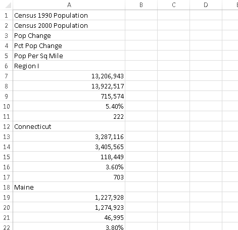
Figure 73-2: Using copy and paste doesn’t work very well.

The data is copied, but it’s all in a single column. I could spend some time and rearrange the data, but there’s a more efficient way to transfer the PDF file data to Excel.

When coping from a PDF file and pasting to a worksheet, the actual results will vary, depending on the layout of the PDF file. In some cases, the pasted text is usable. But in most cases, it’s not.

Using Word 2013 as an intermediary

Excel can’t open PDF files, but Word 2013 can. Figure 73-3 shows a Word document after importing the PDF file. The information can be copied and pasted to an Excel worksheet — and the result will require minimal reformatting (see Figure 73-4).

After making a few minor edits, the table looks perfect.

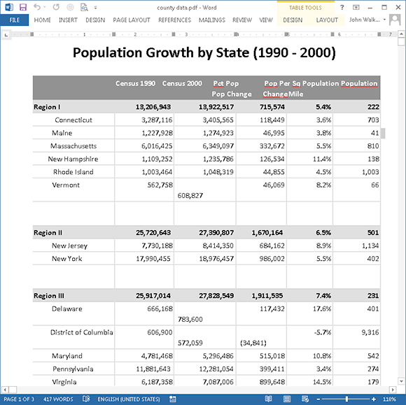
Figure 73-3: A PDF file, imported into World 2013.

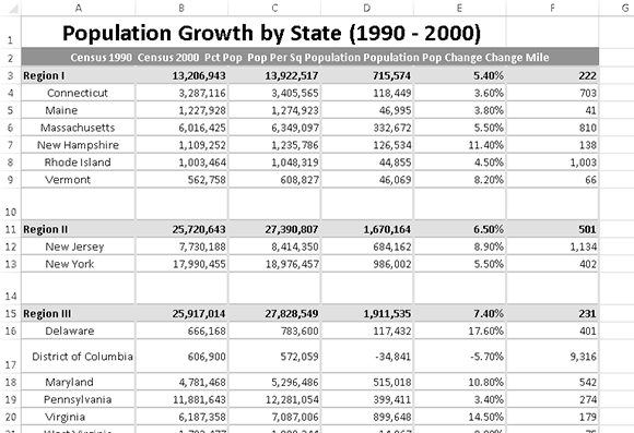
Figure 73-4: A Word 2013 document pasted into an Excel worksheet.

The ability to open PDF files is new to Word 2013, so this method won’t work with other previous versions of Word.