Tip 13: Working with Merged Cells

Merging cells is a simple concept: Join two or more cells to create a larger single cell. To merge cells, just select them and choose Home⇒Alignment⇒Merge & Center. Excel combines the selected cells and displays the contents of the upper-left cell, centered.

Merging cells is usually done as a way to enhance the appearance of a worksheet. Figure 13-1, for example, shows a worksheet with four sets of merged cells: C2:I2, J2:P2, B4:B8, and B9:B13. The merged cells in column B also use vertical text.

Figure 13-1: This worksheet has four sets of merged cells.

Remember that merged cells can contain only one piece of information: a single value, text, or a formula. If you attempt to merge a range of cells that contains more than one nonempty cell, Excel prompts you with a warning that only the data in the upper-leftmost cell will be retained.

To unmerge cells, just select the merged area and click the Merge and Center button again.

Other merge actions

Notice that the Merge and Center button is a drop-down menu. If you click the arrow, you see three additional commands:

→ Merge Across: Lets you select a range and then creates multiple merged cells — one for each row in the selection.

→ Merge Cells: Works just like Merge and Center, except that the content of the upper-left cell is not centered. (It retains its original horizontal alignment.)

→ Unmerge Cells: Unmerges the selected merged cell.

Wrapping text in merged cells is an easy way to display lengthy text. To make text wrap in merged cells, select the merged cells and choose Home⇒Alignment⇒Wrap Text. Use the vertical and horizontal alignment controls in Home⇒Alignment group to adjust the text position.

Figure 13-2 shows a worksheet in which 171 cells have been merged (19 rows and 9 columns). The text in the merged cells uses the Wrap Text option.

Figure 13-2: Here 171 cells are merged into one.

Potential problems with merged cells

Many Excel users have a deep-seated hatred of merged cells. They avoid using this feature and urge everyone else to also avoid merged cells. But if you understand the limitations and potential problems, there’s no reason to completely avoid using merged cells.

Here are a few things to keep in mind:

→ You can’t use merged cells in a table (created by choosing Insert⇒Tables⇒Table). This is understandable because data in a table must be consistent in terms of rows and columns. Merging cells in a table will destroy that consistency.

→ Normally, you can double-click a column header or row header to autofit the data in the column or row, but that feature doesn’t work if the row or column contains merged cells. Instead, you need to adjust the column width or row height manually.

→ Merged cells can also affect sorting and filtering. That’s another reason why merged cells aren’t allowed in tables. If you have a range of data that you will sort or filter, avoid using merged cells.

→ Finally, merged cells can cause problems with VBA macros. For example, if the cells in A1:D1 are merged, a VBA statement such as the following will actually select four columns (not at all what the programmer intended):

Columns(“B:B”).Select

Locating all merged cells

To find out whether a worksheet contains merged cells, follow these steps:

1. Press Ctrl+F to open the Find and Replace dialog box.

2. Check to be sure the Find What field is empty.

3. Click the Options button to expand the dialog box.

4. Click the Format button to open the Find Format dialog box, where you specify the formatting to find.

5. In the Find Format dialog box, choose the Alignment tab and place a check mark next to Merged Cells.

6. Click OK to close the Find Format dialog box.

7. In the Find and Replace dialog box, click Find All.

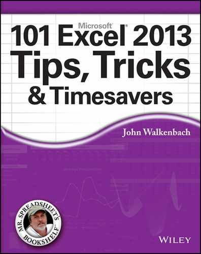
Excel displays a list of all merged cells in the worksheet (see Figure 13-3). Click an address in the list, and the merged cell is activated.

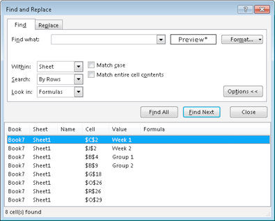
Figure 13-3: Finding all merged cells in a worksheet.

Unmerging all merged cells

Here’s a quick way to unmerge all merged cells in a worksheet:

1. Select all cells in the worksheet.

A quick way to do so is to click the triangle at the intersection of the row headers and column headers.

2. Click the Home tab.

3. If the Merge & Center command is highlighted, click it.

In Step 3, if the Merge & Center command isn’t highlighted, there are no merged cells. If you click the command when all cells are selected, all 17,179,869,184 cells in the worksheet will be merged.

Alternatives to merged cells

In some cases, you can use Excel’s Center Across Selection command as an alternative to merged cells. This command is useful for centering text across several columns.

1. Enter the text to be centered in a cell.

2. Select the cell that has the text and additional cells to the right of it.

3. Press Ctrl+1 to display the Format Cells dialog box.

4. In the Format Cells dialog box, choose the Alignment tab.

5. In the Text Alignment section, choose the Horizontal drop-down and select Center Across Selection.

6. Click OK to close the Format Cells dialog box.

The text is centered across the selected cells.

Another alternative to merging cells is to use a text box. This is particular useful for text that must be displayed vertically. Figure 13-4 shows an example of a text box that displays vertical text. To add a text box, choose Insert⇒Text⇒Text Box, draw the box on the worksheet, and then enter the text. Use the text formatting tools on the Home tab to adjust the text; use the tools in the Drawing Tools⇒Format context tab to make other modifications (for example, to hide the text box outline).

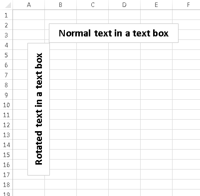
Figure 13-4: Using a text box as an alternative to merged cells.

Tip 14: Indenting Cell Contents

As you probably know, Excel (by default) left-aligns text and right-aligns numbers. Most of the time, that’s exactly how you want data to be aligned.

But if a column of text is to the right of a column of numbers, the information can be difficult to read. Figure 14-1 shows an example. All the data in this table uses the default alignment. The table would be more legible if there were a larger gap between the numbers and the text.

Figure 14-1: The legibility of this table can be improved by indenting the text.

Many users don’t realize that Excel can indent data — either from the left or from the right. Unfortunately, the command to indent is not on the Ribbon. You need to select the cells and then use the Alignment tab of the Format Cells dialog box (see Figure 14-2). A quick way to access this dialog box is to click the dialog launcher icon in the lower-right corner of the Home⇒Alignment group.

Figure 14-2: The Alignment tab of the Format Cells dialog box.

Use the Indent spinner to specify the size of the indenting. Usually, 1 is sufficient, but feel free to experiment. Then use the Horizontal drop-down list to choose the location for the indent: either Left (Indent) or Right (Indent). Click OK, and the text adjusts.

Figure 14-3 shows the original table after indenting the text. Much more legible!

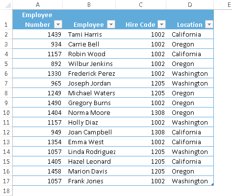
Figure 14-3: Indenting the text makes the table easier to read.

Tip 15: Using Named Styles

Throughout the years, one of the most underused features in Excel has been named styles. Named styles make it very easy to apply a set of predefined formatting options to a cell or range. In addition to saving time, using named styles helps to ensure a consistent look across your worksheets.

A style can consist of settings for up to six different attributes (which correspond to the tabs in the Format Cells dialog box):

→ Number format

→ Alignment (vertical and horizontal)

→ Font (type, size, and color)

→ Borders

→ Fill (background color)

→ Protection (locked and hidden)

The real power of styles is apparent when you change a component of a style. All cells that have been assigned that named style automatically incorporate the change. Suppose that you apply a particular style to a dozen cells scattered throughout your worksheet. Later, you realize that these cells should have a font size of 14 points rather than 12 points. Rather than change each cell, simply edit the style definition. All cells with that particular style change automatically.

Using the Style gallery

Excel comes with dozens of predefined styles, and you apply these styles in the Style gallery (located in the Home⇒Styles group). Figure 15-1 shows the predefined styles in the Style gallery. To apply a style to the selected cell or range, just click the style. Notice that this gallery provides a preview. When you hover your mouse over a style, it’s temporarily applied to the selection so that you can see the effect. To make it permanent, just click the style.

After you apply a style to a cell, you can apply additional formatting to it by using any formatting method discussed in this chapter. Formatting modifications that you make to the cell don’t affect other cells that use the same style.

To maximize the value of styles, it’s best to avoid additional formatting. Rather, consider creating a new style (explained later in this tip).

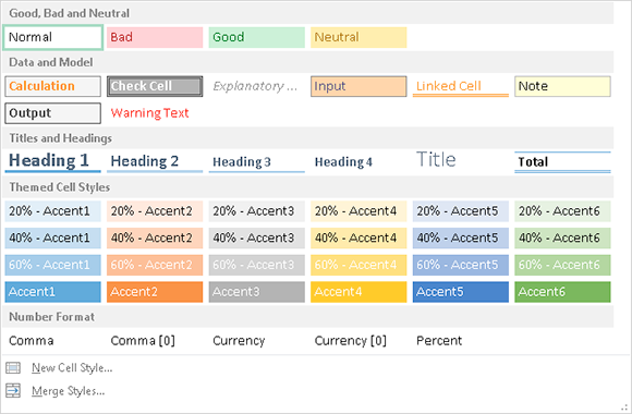
Figure 15-1: Use the Style gallery to work with named styles.

Modifying an existing style

To change an existing style, activate the Style gallery, right-click the style you want to modify, and choose Modify from the shortcut menu. Excel displays the Style dialog box, shown in Figure 15-2. In this example, the Style dialog box shows the settings for the Normal style, which is the default style for all cells. (The style definitions vary, depending on which document theme is active.)

Figure 15-2: Use the Style dialog box to modify named styles.

Cells, by default, use the Normal style. Here’s a quick example of how you can use styles to change the default font used throughout your workbook:

1. Choose Home⇒Styles⇒Cell Styles.

Excel displays the list of styles for the active workbook.

2. Right-click Normal in the Styles list and choose Modify.

The Style dialog box opens with the current settings for the Normal style.

3. Click the Format button.

The Format Cells dialog box opens.

4. Click the Font tab and choose the font and size that you want as the default.

5. Click OK to return to the Style dialog box.

6. Click OK again to close the Style dialog box.

The font for all cells that use the Normal style changes to the font that you specified. You can change any formatting attributes for any style.

Creating new styles

In addition to using the built-in Excel styles, you can create your own styles. This flexibility can be quite handy because it enables you to apply your favorite formatting options very quickly and consistently.

To create a new style from an existing formatted cell, follow these steps:

1. Select a cell and apply all the formatting that you want to include in the new style.

You can use any of the formatting that’s available in the Format Cells dialog box.

2. After you format the cell to your liking, activate the Style gallery and choose New Cell Style.

The Style dialog box opens, along with a proposed generic name for the style. Note that Excel displays the words “By Example” to indicate that it’s basing the style on the current cell.

3. Enter a new style name in the Style Name box.

The check boxes show the current formats for the cell. By default, all check boxes are checked.

4. If you don’t want the style to include one or more format categories, remove the check marks from the appropriate boxes.

5. Click OK to create the style and close the dialog box.

After you perform these steps, the new custom style is available in the Style gallery. Custom styles are available only in the workbook in which they were created. To copy your custom styles, see the section that follows.

The Protection option in the Styles dialog box controls whether users can modify cells for the selected style. This option is effective only if you also turn on worksheet protection, by choosing Review⇒Changes⇒Protect Sheet.

Merging styles from other workbooks

It’s important to understand that custom styles are stored with the workbook in which they were created. If you created some custom styles, you probably don’t want to go through all the work to create copies of those styles in each new Excel workbook. A better approach is to merge the styles from a workbook in which you previously created them.

To merge styles from another workbook, open both the workbook that contains the styles you want to merge and the workbook into which you want to merge styles. From the workbook into which you want to merge styles, activate the Style gallery and choose Merge Styles. The Merge Styles dialog box opens with a list of all open workbooks. Select the workbook that contains the styles you want to merge and click OK. Excel copies styles from the workbook you selected into the active workbook.

You may want to create a master workbook that contains all your custom styles so that you always know from which workbook to merge styles.

Tip 16: Creating Custom Number Formats

Although Excel provides a good variety of built-in number formats, you may find that none of them suits your needs. In such a case, you can probably create a custom number format. You do so on the Number tab of the Format Cells dialog box (see Figure 16-1). The easiest way to display this dialog box is to press Ctrl+1. Or click the dialog box launcher in the Home⇒Number group. (The dialog box launcher is the small icon to the right of the word Number.)

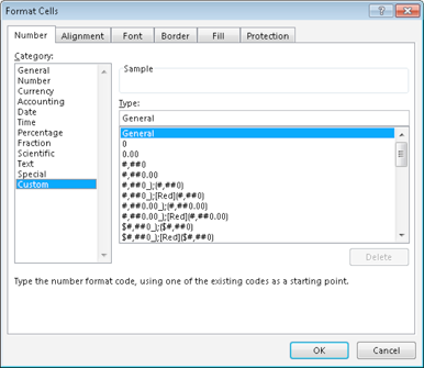
Figure 16-1: Create custom number formats on the Number tab of the Format Cells dialog box.

Many Excel users — even advanced users — avoid creating custom number formats because they think that the process is too complicated. In reality, custom number formats tend to look more complex than they are.

You construct a number format by specifying a series of codes as a number format string. To enter a custom number format, follow these steps:

1. Press Ctrl+1 to display the Format Cells dialog box.

2. Click the Number tab and select the Custom category.

3. Enter your custom number format in the Type field.

See Tables 16-1 and 16-2 for examples of codes you can use to create your own, custom number formats.

4. Click OK to close the Format Cells dialog box.

Parts of a number format string

A custom format string enables you to specify different format codes for four categories of values: positive numbers, negative numbers, zero values, and text. You do so by separating the codes for each category with a semicolon. The codes are arranged in four sections, separated by semicolons:

Positive format; Negative format; Zero format; Text format

The following general guidelines determine how many of these four sections you need to specify:

→ If your custom format string uses only one section, the format string applies to all values.

→ If you use two sections, the first section applies to positive values and zeros, and the second section applies to negative values.

→ If you use three sections, the first section applies to positive values, the second section applies to negative values, and the third section applies to zeros.

→ If you use all four sections, the last section applies to text stored in the cell.

The following example of a custom number format specifies a different format for each of these types:

[Green]General;[Red]-General;[Black]General;[Blue]General

This example takes advantage of the fact that colors have special codes. A cell formatted with this custom number format displays its contents in a different color, depending on the value. When a cell is formatted with this custom number format, a positive number is green, a negative number is red, a zero is black, and text is blue. By the way, using the Excel conditional formatting feature is a much better way to apply color to cells based on their content.

When you create a custom number format, don’t overlook the Sample box in the Number tab of the Format Cells dialog box. This box displays the value in the active cell by using the format string in the Type field. Be sure to test your custom number formats by using the following data: a positive value, a negative value, a zero value, and text. Often, creating a custom number format takes several attempts. Each time you edit a format string, it’s added to the list. When you finally get the correct format string, open the Format Cells dialog box one more time and delete your previous attempts.

Custom number format codes

Table 16-1 briefly describes the formatting codes available for custom formats.

Table 16-1: Codes Used to Create Custom Number Formats

Code	What It Does
General	Displays the number in General format.
#	Serves as a digit placeholder that displays only significant digits and doesn’t display insignificant zeros.
0 (zero)	Serves as a digit placeholder that displays insignificant zeros if a number has fewer digits than there are zeros in the format.
?	Serves as a digit placeholder that adds spaces for insignificant zeros on either side of the decimal point so that decimal points align when formatted with a fixed-width font; also used for fractions that have varying numbers of digits.
.	Displays the decimal point.
%	Displays a percentage.
,	Displays the thousands separator.
E- E+ e- e+	Displays scientific notation.
$ – + / ( ) : space	Displays the actual character.
	Displays the next character in the format.
*	Repeats the next character to fill the column width.
_ (underscore)	Leaves a space equal to the width of the next character.
“text”	Displays the text inside the double quotation marks.
@	Serves as a text placeholder.
[color]	Displays the characters in the specified color and can be any of the following text strings (not case-sensitive): Black, Blue, Cyan, Green, Magenta, Red, White, or Yellow.
[COLOR n]	Displays the corresponding color in the color palette, where n is a number from 0 to 56.
[condition value]	Enables you to set your own criteria for each section of a number format.

Table 16-2 describes the codes used to create custom formats for dates and times.

Table 16-2: Codes Used in Creating Custom Formats for Dates and Times

Code	What It Displays
M	The month as a number without leading zeros (1–12)
mm	The month as a number with leading zeros (01–12)
mmm	The month as an abbreviation (Jan–Dec)
mmmm	The month as a full name (January–December)
mmmmm	The first letter of the month (J–D)
d	The day as a number without leading zeros (1–31)
dd	The day as a number with leading zeros (01–31)
ddd	The day as an abbreviation (Sun–Sat)
dddd	The day as a full name (Sunday–Saturday)
yy or yyyy	The year as a two-digit number (00–99) or as a four-digit number (1900–9999)
h or hh	The hour as a number without leading zeros (0–23) or as a number with leading zeros (00–23)
m or mm	The minute as a number without leading zeros (0–59) or as a number with leading zeros (00–59)
s or ss	The second as a number without leading zeros (0–59) or as a number with leading zeros (00–59)
[ ]	Hours greater than 24 or minutes or seconds greater than 60
AM/PM	The hour using a 12-hour clock or no AM/PM indicator if the hour uses a 24-hour clock

Tip 17: Using Custom Number Formats to Scale Values

If you work with large numbers, you may prefer to display them scaled to thousands or millions rather than display the entire number. For example, you may want to display a number like 132,432,145 in millions: 132.4.

The way to display scaled numbers is to use a custom number format. The actual unscaled number, of course, will be used in calculations that involve that cell. The formatting affects only how the number is displayed. To enter a custom number format, press Ctrl+1 to display the Format Cells dialog box. Then click the Number tab and select the Custom category. Put your custom number format in the Type field.

Table 17-1 shows examples of number formats that scale values in millions.

Table 17-1: Examples of Displaying Values in Millions

Value	Number Format	Display
123456789	#,###,,	123
1.23457E+11	#,###,,	123,457
1000000	#,###,,	1
5000000	#,###,,	5
–5000000	#,###,,	–5
0	#,###,,	(blank)
123456789	#,###.00,,	123.46
1.23457E+11	#,###.00,,	123,457.00
1000000	#,###.00,,	1.00
5000000	#,###.00,,	5.00
–5000000	#,###.00,,	–5.00
0	#,###.00,,	.00
123456789	#,###,,”M”	123M
1.23457E+11	#,###,,”M”	123,457M
1000000	#,###,,”M”	1M
–5000000	#,###,,”M”	–5M
123456789	#,###.0,,”M”_);(#,###.0,,”M)”;0.0”M”_)	123.5M
1000000	#,###.0,,”M”_);(#,###.0,,”M)”;0.0”M”_)	1.0M
–5000000	#,###.0,,”M”_);(#,###.0,,”M)”;0.0”M”_)	(5.0M)
0	#,###.0,,”M”_);(#,###.0,,”M)”;0.0”M”_)	0.0M

Table 17-2 shows examples of number formats that scale values in thousands.

Table 17-2: Examples of Displaying Values in Thousands

Value	Number Format	Display
123456	#,###,	123
1234565	#,###,	1,235
–323434	#,###,	–323
123123.123	#,###,	123
499	#,###,	(blank)
500	#,###,	1
500	#,###.00,	.50

Table 17-3 shows examples of number formats that display values in hundreds.

Table 17-3: Examples of Displaying Values in Hundreds

Value	Number Format	Display
546	0”.”00	5.46
100	0”.”00	1.00
9890	0”.”00	98.90
500	0”.”00	5.00
–500	0”.”00	–5.00
0	0”.”00	0.00

Tip 18: Creating a Bulleted List

Word-processing software, such as Microsoft Word, makes it very easy to create a bulleted list of items. Excel doesn’t have a feature that creates bulleted lists, but it’s easy to fake it.

Using a bullet character

You can generate a bullet character by pressing Alt, and typing 0149 on the numeric keypad. If your keyboard lacks a numeric keypad, press the Function key and type numbers using the normal keys.

Figure 18-1 shows a list in which each item is preceded with a bullet character and a space. The cells use wrap-text formatting. Items that occupy more than one line are not indented. In a bulleted list, multiple lines are usually indented so they line up with the first line.

Figure 18-1: Inserting a bullet character before each item.

Figure 18-2 shows a second attempt. This approach requires two columns. Column A holds the bullet character, formatted so the bullet is top-aligned and right-aligned. The text is in column B.

Figure 18-2 also shows an alternative, a numbered list. The cells that contain the numbers use this custom number format, which displays a decimal point, but no decimal places:

General”. “

You can, of course, use any character you like for the bullet. Use Insert⇒Symbols➜Symbol to display (and insert) characters from any font that’s installed on your system.

Figure 18-2: Using an additional column for the bullet characters, or for numbers.

Using SmartArt

Another way to create a bulleted list in Excel is to use SmartArt. Choose Insert⇒Illustrations➜SmartArt, and choose the diagram style from the dialog box.

Figure 18-3 shows a “Vertical Bullet List” SmartArt diagram. This object is free-floating and can easily be moved and resized. The example shown here uses minimal formatting, but you have lots of control over the appearance of SmartArt.

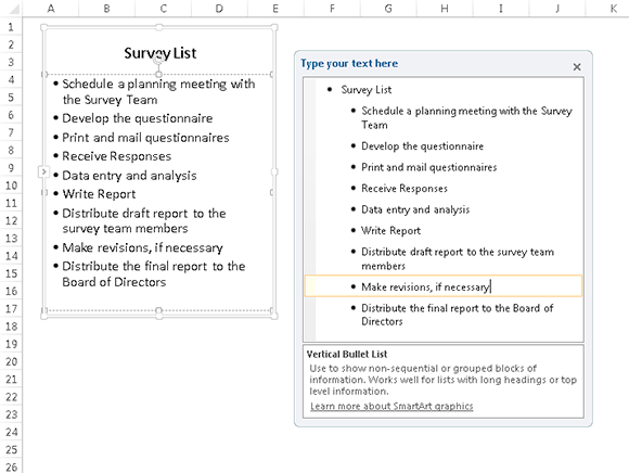
Figure 18-3: Using SmartArt to hold a bulleted list.

Tip 19: Shading Alternate Rows Using Conditional Formatting

When you create a table (using Insert⇒Tables⇒Table), you have the option of formatting the table in such a way that alternate rows are shaded. Alternate row shading can make your spreadsheets easier to read.

This tip describes how to use conditional formatting to obtain alternate row shading for any range of data. It’s a dynamic technique: If you add or delete rows within the conditional formatting area, the shading is updated automatically.

Displaying alternate row shading

Figure 19-1 shows an example. Here’s how to apply shading to alternate rows:

1. Select the range to format.

2. Choose Home⇒Conditional Formatting⇒New Rule.

The New Formatting Rule dialog box appears.

3. For the rule type, choose Use a Formula to Determine Which Cells to Format.

4. Enter the following formula in the box labeled Format Values Where This Formulas Is True:

=MOD(ROW(),2)=0

5. Click the Format button.

The Format Cells dialog box appears.

6. In the Format Cells dialog box, click the Fill tab and select a background fill color.

7. Click OK to close the Format Cells dialog box, and click OK again to close the New Formatting Rule dialog box.

This conditional formatting formula uses the ROW function (which returns the row number) and the MOD function (which returns the remainder of its first argument divided by its second argument). For cells in even-numbered rows, the MOD function returns 0, and cells in that row are formatted.

For alternate shading of columns, use the COLUMN function instead of the ROW function.

Figure 19-1: Using conditional formatting to apply formatting to alternate rows.

Creating checkerboard shading

The following formula is a variation on the example in the preceding section. It applies formatting to alternate rows and columns, creating a checkerboard effect. Figure 19-2 shows the result.

=MOD(ROW(),2)=MOD(COLUMN(),2)

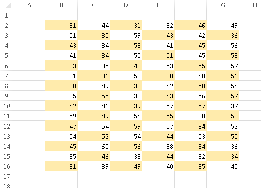
Figure 19-2: Conditional formatting produces this checkerboard effect.

Shading groups of rows

Here’s another row shading variation. The following formula shades alternate groups of rows. It produces four rows of shaded rows, followed by four rows of unshaded rows, followed by four more shaded rows, and so on. Figure 19-3 shows an example.

=MOD(INT((ROW()-1)/4)+1,2)

For different sized groups, change the 4 to some other value. For example, use this formula to shade alternate groups of two rows:

=MOD(INT((ROW()-1)/2)+1,2)

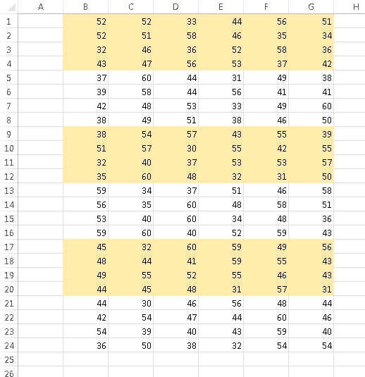
Figure 19-3: Conditional formatting produces these groups of alternate shaded rows.

Tip 20: Formatting Individual Characters in a Cell

Excel cell formatting isn’t an all-or-none proposition. In some cases, you might find it helpful to be able to format individual characters within a cell.

This technique is limited to cells that contain text. It doesn’t work if the cell contains a value or a formula.

To apply formatting to characters within a text string, select those characters first. You can select them by clicking and dragging your mouse on the Formula bar, or you can double-click the cell and then click and drag the mouse to select specific characters directly in the cell. A more efficient way to select individual characters is to press F2 first and then use the arrow keys to move between characters and use the Shift+arrow keys to select characters.

When the characters are selected, use formatting controls to change the formatting. For example, you can make the selected text bold, italic, or a different color; you can even apply a different font. If you right-click, the Mini Toolbar appears, and you can use those controls to change the formatting of the selected characters.

Figure 20-1 shows a few examples of cells that contain individual character formatting.

Unfortunately, two useful formatting attributes are not available on the Ribbon or on the Mini Toolbar: superscript and subscript formatting. If you want to apply superscripts or subscripts, open the Font tab in the Format Cells dialog box. Just press Ctrl+1 after you select the text to format.

Figure 20-1: Examples of individual character formatting.

Tip 21: Using the Format Painter

You’ve probably seen that little Format Painter paint brush icon in the Home⇒Clipboard group. It’s an easy way to copy cell formatting — and it’s actually more versatile than you might think.

When you use the Format Painter, every aspect of the source range’s formatting is copied, including number formats, borders, cell merging, and conditional formatting.

Painting basics

Here’s how to use the Format Painter tool in its basic form:

1. Select a cell that contains the formatting that you want to duplicate.

2. Choose Home⇒Clipboard⇒Format Painter.

The mouse cursor displays a paintbrush to remind you that you’re in Format Painter mode (see Figure 21-1).

3. Drag the mouse over another range.

4. Release the mouse button, and the formatting is copied.

In Step 2, you can right-click the selected cell and choose the Format Painter icon from the Mini Toolbar.

Note that the Format Painter is mouse-centric. You cannot use the keyboard to do your painting.

Figure 21-1: Copying cell formatting by using the Format Painter.

Format Painter variations

In Step 1 in the preceding section, if you select a range of cells, you can paint another range by clicking a single cell. The formatting is copied to a range that’s the same size as the original selection.

In Step 2, if you double-click the Format Painter button, Excel remains in Format Painter mode until you cancel it. This enables you to copy the format to multiple ranges of cells. To get out of Format Painter mode, press Esc or click the Format Painter button again.

You can also use the Format Painter to remove all formatting from a range and return the range to its pristine state. Start by selecting an unformatted cell. Then click the Format Painter button and drag it over the range.

The Format Painter also works with complete rows and columns. If you start by selecting one or more complete rows, the Format Painter also copies row height. The same thing occurs with column widths if you start by selecting one or more columns.

This feature even works with complete worksheets. For example, if you want to remove all formatting from a worksheet, select an unformatted cell, click the Format Painter button, and then click the “select all” button at the intersection of the row and column borders.

You can also use the Format Painter with shapes and other objects such as pictures. Just select the object, click the Format Painter button, and click another object. Figure 21-2 shows an example of copying shape formats using the Format Painter.

Although the Format Painter is versatile, it doesn’t work with charts.

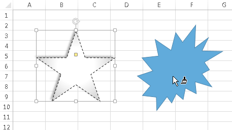
Figure 21-2: Using the Format Painter to copy shape formatting.

Finally, the Format Painter is a handy tool, but it doesn’t perform any actions that can’t be done via other methods. For example, you can copy a range, select another range, and use the Home➜Clipboard⇒Paste⇒Formatting (R) command to paste the formatting only.

Tip 22: Inserting a Watermark

A watermark is an image (or text) that appears on a printed page. A watermark can be a faint company logo or a word, such as DRAFT.

Excel doesn’t have an official command to print a watermark, but you can add a watermark by inserting a picture in the page header or footer. Here’s how to do it:

1. Locate an image on your hard drive that you want to use for the watermark.

2. Choose View⇒Workbook Views⇒Page Layout View to enter Page Layout view.

3. Click the center section of the header.

4. Choose Header & Footer Tools⇒Header & Footer Elements⇒Picture.

The Insert Picture dialog box appears.

5. Click Browse and locate and select the image you picked in Step 1 (or locate a suitable image from other sources listed); then click Insert to insert the image.

6. Click outside the header to see your image.

7. To center the image vertically on the page, click the center section of the header and press Enter a few times before the &[Picture] code.

You’ll need to experiment to determine the number of carriage returns required to push the image into the body of the document.

8. If you need to adjust the image (for example, to make it lighter), click the center section of the header and then choose Header & Footer Tools⇒Header & Footer Elements⇒Format Picture; use the Image controls on the Picture tab of the Format Picture dialog box to adjust the image.

You may need to experiment with the settings to make sure that the worksheet text is legible.

Figure 22-1 shows an example of a header image (a copyright symbol) used as a watermark. You can create a similar effect with plain text in the header (for example, the word DRAFT).

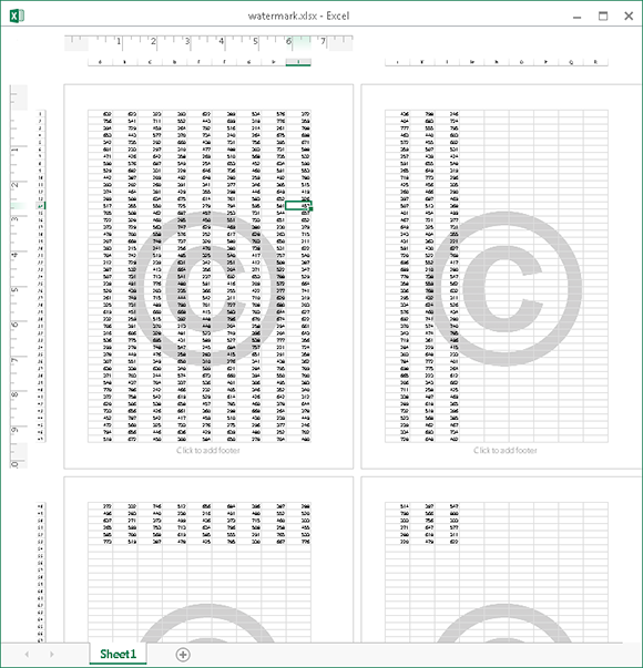
Figure 22-1: Displaying a watermark on a page.

Tip 23: Showing Text and a Value in a Cell

If you need to display a number and text in a single cell, Excel gives you three options:

→ Concatenation

→ The TEXT function

→ A custom number format

Assume that cell A1 contains a value, and in a cell somewhere else in your worksheet, you want to display the text Total: along with that value. It looks something like this:

Total: 594.34

You could, of course, put the text Total: in the cell to the left. This section describes the three methods for accomplishing this task using a single cell.

Using concatenation

The following formula concatenates the text Total: with the value in cell A1:

=”Total: “&A1

This solution is the simplest, but it has a problem. The result of the formula is text, rather than a numeric value. Therefore, the cell cannot be used in a numeric formula. Also, the numeric portion will display with no formatting. For example, the formula might return

Total: 1594.34320933

Using the TEXT function

Another solution uses the TEXT function, which displays a value by using a specified number format:

=TEXT(A1,”””Total: “”$#,0.00”)

This formula returns something like this:

Total: $1,594.34

The second argument for the TEXT function is a number format string — the same type of string that you use when you create a custom number format. Because the number portion is formatted, this approach looks good. But besides being a bit unwieldy (because of the extra quotation marks), this formula suffers from the same problem mentioned in the previous section: The result is not numeric.

Using a custom number format

If you want to display text and a value — and still be able to use that value in a numeric formula — the solution is to use a custom number format.

To add text, just create the number format string as usual and put the text within quotation marks. For this example, the following custom number format does the job:

“Total: “$#,0.00

Even though the cell displays text, Excel still considers the cell contents to be a numeric value. Therefore, you can use this cell in other formulas that perform calculations.

Tip 24: Avoiding Font Substitution for Small Point Sizes

When you specify a font size smaller than eight points, you may notice that the numbers in a column no longer line up correctly. That’s because Excel uses a different (non-proportional) font for small text. Normally, each numeric character takes the same amount of horizontal space — that’s why numbers line up so nicely. But with a proportional font, numeric characters vary in width. The “1” character is more narrow than the “0” character, for example.

Figure 24-1 shows a worksheet with columns of numbers in varying font sizes. Notice that everything is fine until the point size is smaller than 8 points. In column E (7 points), the “1” character take up less space. In column F (6 points), the “5” and “7” characters also take up less space.

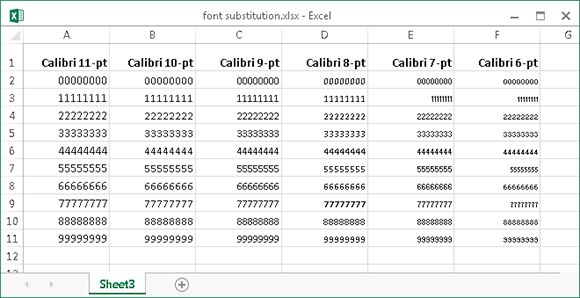
Figure 24-1: Various font sizes, with font substitution enabled.

Font substitution also occurs when you zoom the worksheet, using the Zoom slider in the status bar. Sometimes zooming out causes values to appear as a series of hash marks (#####). The point at which the font is changed seems to vary, depending on the size of the original font. For the default 11-point font, zooming below 75% causes Excel to switch to a different font.

You can instruct Excel to stop this font substitution for small font sizes, but doing so requires editing the Windows registry.

Editing the registry can be dangerous if you don’t understand what you’re doing; always create a backup before you make any changes. If you’re not comfortable editing the registry, find someone who is — or just don’t implement this tip.

1. Close Excel.

2. Click the Windows Start button and run regedit.exe, the Registry Editor program.

3. In the Registry Editor, navigate to this registry key:

HKEY_CURRENT_USERSoftwareMicrosoftOffice15.0ExcelOptions

4. With that registry key selected, choose Edit⇒New⇒DWORD.

The entry will be named New Value #1.

5. Right-click the entry and choose Rename. Specify FontSub for the entry name.

6. Double-click the FontSub entry.

The Edit DWORD dialog box appears.

7. Specify 0 as the Value Data (the Base, Hexadecimal, or Decimal doesn’t matter), as shown in Figure 24-2.

8. Click OK to close the Edit DWORD dialog box.

9. Choose File⇒Exit to quit Registry Editor.

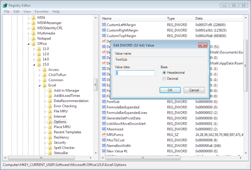
Figure 24-2: Using Registry Editor to add a new value to the Windows registry.

When you restart Excel, you’ll find that Excel no longer uses font substitution for small fonts. When font substitution is disabled, small text will be a bit more difficult to read, but the numbers will continue to line up, and you won’t see the #### display when you zoom out.

Figure 24-3 shows the worksheet in Figure 24-1, after disabling font substitution.

Figure 24-3: Various font sizes, with font substitution disabled.

Tip 25: Updating Old Fonts

When you install Microsoft Office, several new fonts are added to your system, and these new fonts are used when you create a new workbook. The exact fonts that are used as defaults vary, depending on which document theme is in effect.

  See Tip 10 for more information about using document themes.

If you use the default Office theme, a newly created Excel workbook uses two new fonts: Cambria (for headings) and Calibri (for body text). When you open a workbook that was saved in a version prior to Excel 2007, the old fonts (probably Arial) aren’t updated. The difference in appearance between a worksheet that uses the old fonts and a worksheet that uses the new fonts is dramatic. When you compare an Excel 2003 worksheet with an Excel 2013 worksheet, the latter is much more readable and appears less cramped.

Figure 25-1 shows a workbook that was created in Excel 2003.

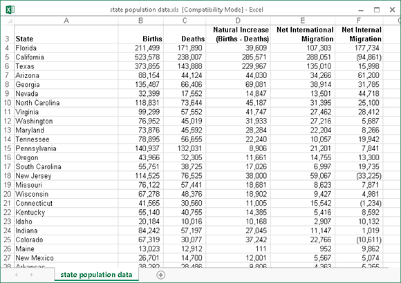
Figure 25-1: This Excel 2003 workbook uses Arial 10-point font as the normal font.

To update the fonts in a workbook that was created in a previous version of Excel, follow these steps:

1. Press Ctrl+N to create a new, blank workbook.

2. Activate the workbook that uses the fonts to be updated.

3. Choose Home⇒Styles⇒Merge Styles

The Merge Styles dialog box appears.

4. In the Merge Styles dialog box, select the workbook that you created in Step 1 and click OK.

Excel asks whether you want to merge styles that have the same names.

5. Reply by clicking the Yes button.

This procedure updates the fonts used in all cells except those that have additional formatting, such as a different font size, bold, italic, colored text, or a shaded background. To change the font in these cells, follow these steps:

1. Select any single cell.

2. Choose Home⇒Editing⇒Find & Select⇒Replace, or press Ctrl+H.

The Find and Replace dialog box appears.

3. Make sure that the two Format buttons are visible. If these buttons aren’t visible, click the Options button to expand the dialog box.

4. Click the upper Format button to display the Find Format dialog box.

5. Click the Font tab.

6. In the Font list, select the name of the font that you’re replacing (probably Arial, the old default font) and then click OK to close the Find Format dialog box.

7. Click the lower Format button to display the Replace Format dialog box.

8. Click the Font tab.

9. In the Font list, select the name of the font that will replace the old font (probably Calibri) and then click OK to close the Replace Format dialog box.

10. In the Find and Replace dialog box, click Replace All to replace the old font with the new font.

Figure 25-2 shows the Excel 2003 workbook after updating the font.

Figure 25-2: This Excel workbook uses Calibri 11-point font as the normal font.