One of the most important things you do in Excel is navigating the worksheet. When you work with Excel manually, you are constantly navigating to appropriate ranges, finding the last row, moving to the last column, hiding and unhiding ranges, and so on. This all comes instinctively as part of doing work in Excel.
When you attempt to automate your work through VBA, you'll find that navigating your spreadsheet remains an important part of the automation process. In many cases, you need to dynamically navigate and manipulate Excel ranges, just as you would manually — only through VBA code. This chapter provides some of the most commonly used macros in terms of navigating and working with ranges.
 The code for this Part can be found on this book's companion website. See this book's Introduction for more on the companion website.
Macro 31: Selecting and Formatting a Range
One of the basic things you need to do in VBA is to select a specific range to do something with it. This simple macro selects the range D5:D16.
How it works
In this macro, you explicitly define the range to select by using the Range object.
Sub Macro31a()
Range(“D5:D16”).Select
End Sub
After the range of cells is selected, you can use any of the Range properties to manipulate the cells. We've altered this macro so that the range is colored yellow, converted to number formatting, and bold.
Sub Macro31a()
Range(“D5:D16”).Select
Selection.NumberFormat = “#,##0”
Selection.Font.Bold = True
Selection.Interior.ColorIndex = 36
End Sub
You don't have to memorize all the properties of the cell object in order to manipulate them. You can simply record a macro, do your formatting, and then look at the code that Excel has written. After you've seen what the correct syntax is, you can apply it as needed. Many Excel programmers start learning VBA this way.
You notice that we refer to Selection many times in the previous sample code. To write more efficient code, you can simply refer to the range, using the With…End With statement. This statement tells Excel that any action you perform applies to the object to which you've pointed. Note that this macro doesn't actually select the range at all. This is a key point. In a macro, we can work with a range without selecting it first.
Sub Macro31a()
With Range(“D5:D16”)
.NumberFormat = “#,##0”
.Font.Bold = True
.Interior.ColorIndex = 36
End With
End Sub
Another way you can select a range is by using the Cells item of the Range object.
The Cells item gives us an extremely handy way of selecting ranges through code. It requires only relative row and column positions as parameters. Cells(5, 4) translates to row 5, column 4 (or Cell D5). Cells(16, 4) translates to row 16, column 4 (or cell D16).
If you want to select a range of cells, simply pass two items into the Range object. This macro performs the same selection of range D5:D16:
Sub Macro31a()
Range(Cells(5, 4), Cells(16, 4)).Select
End Sub
Here is the full formatting code using the Cells item. Again, note that this macro doesn't actually select the range we are altering. We can work with a range without selecting it first.
Sub Macro31a()
With Range(Cells(5, 4), Cells(16, 4))
.NumberFormat = “#,##0”
.Font.Bold = True
.Interior.ColorIndex = 36
End With
End Sub
How to use it
To implement this kind of a macro, you can copy and paste it into a standard module:
1. Activate the Visual Basic Editor by pressing ALT+F11 on your keyboard.
2. Right-click the project/workbook name in the Project window.
3. Choose Insert⇒Module.
4. Type or paste the code into the code window.
Macro 32: Creating and Selecting Named Ranges
One of the more useful features in Excel is the ability to name your range (that is, to give your range a user-friendly name, so that you can more easily identify and refer to it via VBA).
Here are the steps you would perform to create a named range manually.
1. Select the range you wish to name.
2. Go to the Formulas tab in the Ribbon and choose the Define Name command (see Figure 4-1).
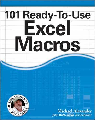
3. Give the chosen range a user-friendly name in the New Name dialog box, as shown in Figure 4-2.
When you click OK, your range is named. To confirm this, you can go to the Formula tab and select the Name Manager command. This activates the Name Manager dialog box (see Figure 4-3), where you can see all the applied named ranges.

Figure 4-1: Click the Define Name command to name a chosen range.
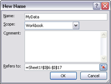
Figure 4-2: Give your range a name.
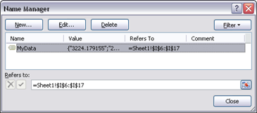
Figure 4-3: The Name Manager dialog box lists all the applied named ranges.
Creating a named range via VBA is much less involved. You can directly define the Name property of the Range object:
Sub Macro32a()
Range(“D6:D17”).Name = “MyData”
End Sub
Admittedly, you'd be hard pressed to find a situation where you would need to automate the creation of named ranges. The real efficiency comes in manipulating them via VBA.
How it works
You simply pass the name of the range through the Range object. This allows you to select the range:
Sub Macro32b()
Range(“MyData”).Select
End Sub
As with normal ranges, you can refer to the range using the With…End With statement. This statement tells Excel that any action you perform applies to the object to which you've pointed. This not only prevents you from having to repeat syntax, but it also allows for the easy addition of actions by simply adding them between the With and End With statements.
Sub Macro32a()
With Range(“MyData”)
.NumberFormat = “#,##0”
.Font.Bold = True
.Interior.ColorIndex = 36
End With
End Sub
How to use it
To implement this kind of a macro, you can copy and paste it into a standard module:
1. Activate the Visual Basic Editor by pressing ALT+F11.
2. Right-click the project/workbook name in the Project window.
3. Choose Insert⇒Module.
4. Type or paste the code.
Macro 33: Enumerating Through a Range of Cells
One must-have VBA skill is the ability to enumerate (or loop) through a range. If you do any serious macro work in Excel, you will soon encounter the need to go through a range of cells one by one and perform some action.
This basic macro shows you a simple way to enumerate through a range.
How it works
In this macro, we are essentially using two Range object variables. One of the variables captures the scope of data we are working with, whereas the other is used to hold each individual cell as we go through the range. Then we use the For Each statement to activate or bring each cell in the target range into focus:
Sub Macro33()
‘Step1: Declare your variables.
Dim MyRange As Range
Dim MyCell As Range
‘Step 2: Define the target Range.
Set MyRange = Range(“D6:D17”)
‘Step 3: Start looping through the range.
For Each MyCell In MyRange
‘Step 4: Do something with each cell.
If MyCell.Value > 3000 Then
MyCell.Font.Bold = True
End If
‘Step 5: Get the next cell in the range
Next MyCell
End Sub
1. The macro first declares two Range object variables. One, called MyRange, holds the entire target range. The other, called MyCell, holds each cell in the range as the macro enumerates through them one by one.
2. In Step 2, we fill the MyRange variable with the target range. In this example, we are using Range(“D6:D17”). If your target range is a named range, you could simply enter its name — Range(“MyNamedRange”).
3. In this step, the macro starts looping through each cell in the target range, activating each cell as it goes through.
4. After a cell is activated, you would do something with it. That “something” really depends on the task at hand. You may want to delete rows when the active cell has a certain value, or you may want to insert a row between each active cell. In this example, the macro is changing the font to Bold for any cell that has a value greater than 3,000.
5. In Step 5, the macro loops back to get the next cell. After all cells in the target range are activated, the macro ends.
How to use it
To implement this macro, you can copy and paste it into a standard module:
1. Activate the Visual Basic Editor by pressing ALT+F11 on your keyboard.
2. Right-click the project/workbook name in the Project window.
3. Choose Insert⇒Module.
4. Type or paste the code.
Macro 34: Select and Format All Named Ranges
If you spend your time auditing other people's worksheets, you'll know that Excel users love their named ranges. It's not uncommon to encounter spreadsheets where dozens of cells and ranges are given individual names. This makes auditing a spreadsheet an extremely muddy experience. It sometimes helps to know where the named ranges are. Here is a macro you can use to color all of the named ranges in a workbook yellow.
How it works
In this macro, we are looping through the Names collection of the active workbook to capture each named range. When a named range is captured, we color the range.
Sub Macro34()
‘Step 1: Declare your variables.
Dim RangeName As Name
Dim HighlightRange As Range
‘Step 2: Tell Excel to Continue if Error.
On Error Resume Next
‘Step 3: Loop through each Named Range.
For Each RangeName In ActiveWorkbook.Names
‘Step 4: Capture the RefersToRange
Set HighlightRange = RangeName.RefersToRange
‘Step 5: Color the Range
HighlightRange.Interior.ColorIndex = 36
‘Step 6: Loop back around to get the next range
Next RangeName
End Sub
1. We first declare two object variables. The first variable called RangeName holds each named range as the macro enumerates through the Names collection. The second variable called HighlightRange captures the range to which RangeName is referring.
2. Technically, an Excel user can assign a “name” to things that are not actually a range (such as constants or formulas). So with that in mind, we have to anticipate that Excel will throw an error if the RefersToRange property of the named range does not represent a range address. In this step, we tell Excel to ignore any error that is thrown and continue to the next line of code. This ensures that the code doesn't abruptly stop due to a bad range address.
3. In this step, the macro starts looping through each name in the active workbooks Names collection.
4. After a named range is activated, the macro captures the address in our HighlightRange object variable. This exposes all the properties we can use to format the range.
5. In Step 5, we assign a color to the cells in the captured range.
6. Finally, we loop back to get the next named range. The macro ends after we have enumerated through all of the names.
How to use it
The best place to store this macro is in your Personal Macro Workbook. This way, the macro is always available to you. The Personal Macro Workbook is loaded whenever you start Excel. In the VBE Project window, it will be named personal.xlb.
1. Activate the Visual Basic Editor by pressing ALT+F11.
2. Right-click personal.xlb in the Project window.
3. Choose Insert⇒Module.
4. Type or paste the code.
If you don't see personal.xlb in your project window, it doesn't exist yet. You'll have to record a macro, using Personal Macro Workbook as the destination.
To record the macro in your Personal Macro Workbook, select the Personal Macro Workbook option in the Record Macro dialog box before you start recording. This option is in the Store Macro In drop-down list. Simply record a couple of cell clicks and then stop recording. You can discard the recorded macro and replace it with this one.
Macro 35: Inserting Blank Rows in a Range
Occasionally, you may need to dynamically insert rows into your dataset. Although blank rows are generally bothersome, in some situations, the final formatted version of your report requires them to separate data. The macro in this section adds blank rows into a range.
How it works
This macro performs a reverse loop through the chosen range using a counter. It starts at the last row of the range inserting two blank rows, and then moves to the previous row in the range. It keeps doing that same insert for every loop, each time incrementing the counter to the previous row.
Sub Macro35()
‘Step1: Declare your variables.
Dim MyRange As Range
Dim iCounter As Long
‘Step 2: Define the target Range.
Set MyRange = Range(“C6:D17”)
‘Step 3: Start reverse looping through the range.
For iCounter = MyRange.Rows.Count To 2 Step -1
‘Step 4: Insert two blank rows.
MyRange.Rows(iCounter).EntireRow.Insert
MyRange.Rows(iCounter).EntireRow.Insert
‘Step 5: Increment the counter down
Next iCounter
End Sub
1. We first declare two variables. The first variable is an object variable called MyRange. This is an object variable that defines the target range. The other variable is a Long Integer variable called iCounter. This variable serves as an incremental counter.
2. In Step 2, the macro fills the MyRange variable with the target range. In this example, we are using Range(“C6:D17”). If your target range is a named range, you could simply enter its name — Range(“MyNamedRange”).
3. In this step, the macro sets the parameters for the incremental counter to start at the max count for the range (MyRange.Rows.Count) and end at 2 (the second row of the chosen range). Note that we are using the Step-1 qualifier. Because we specify Step -1, Excel knows we are going to increment the counter backwards, moving back one increment on each iteration. In all, Step 3 tells Excel to start at the last row of the chosen range, moving backward until it gets to the second row of the range.
4. When working with a range, you can explicitly call out a specific row in the range by passing a row index number to the Rows collection of the range. For instance, Range(“D6:D17”).Rows(5) points to the fifth row in the range D6:D17.
In Step 4, the macro uses the iCounter variable as an index number for the Rows collection of MyRange. This helps pinpoint which exact row the macro is working with in the current loop. The macro then uses the EntireRow.Insert method to insert a new blank row. Because we want two blank rows, we do this twice.
5. In Step 5, the macro loops back to increment the counter down.
How to use it
To implement this macro, you can copy and paste it into a standard module:
1. Activate the Visual Basic Editor by pressing ALT+F11.
2. Right-click the project/workbook name in the Project window.
3. Choose Insert⇒Module.
4. Type or paste the code.
Macro 36: Unhide All Rows and Columns
When you are auditing a spreadsheet that you did not create, you often want to ensure you're getting a full view of what is exactly in the spreadsheet. To do so, you need to ensure that no columns and rows are hidden. This simple macro automatically unhides all rows and columns for you.
How it works
In this macro, we call on the Columns collection and the Rows collection of the worksheet. Each collection has properties that dictate where their objects are hidden or visible. Running this macro unhides every column in the Columns collection and every row in the Rows collection.
Sub Macro36()
Columns.EntireColumn.Hidden = False
Rows.EntireRow.Hidden = False
End Sub
How to use it
The best place to store this macro is in your Personal Macro Workbook. This way, the macro is always available to you. The Personal Macro Workbook is loaded whenever you start Excel. In the VBE Project window, it is named personal.xlb.
1. Activate the Visual Basic Editor by pressing ALT+F11.
2. Right-click personal.xlb in the Project window.
3. Choose Insert⇒Module.
4. Type or paste the code.
If you don't see personal.xlb in your project window, it means it doesn't exist yet. You'll have to record a macro, using Personal Macro Workbook as the destination.
To record the macro in your Personal Macro Workbook, select the Personal Macro Workbook option in the Record Macro dialog box before you start recording. This option is in the Store Macro In drop-down list. Simply record a couple of cell clicks and then stop recording. You can discard the recorded macro and replace it with this one.
Macro 37: Deleting Blank Rows
Work with Excel long enough, and you'll find out that blank rows can often cause havoc on many levels. They can cause problems with formulas, introduce risk when copying and pasting, and sometimes cause strange behaviors in PivotTables. If you find that you are manually searching out and deleting blank rows in your data sets, this macro can help automate that task.
How it works
In this macro, we are using the UsedRange property of the Activesheet object to define the range we are working with. The UsedRange property gives us a range that encompasses the cells that have been used to enter data. We then establish a counter that starts at the last row of the used range to check if the entire row is empty. If the entire row is indeed empty, we remove the row. We keep doing that same delete for every loop, each time incrementing the counter to the previous row.
Sub Macro37()
‘Step1: Declare your variables.
Dim MyRange As Range
Dim iCounter As Long
‘Step 2: Define the target Range.
Set MyRange = ActiveSheet.UsedRange
‘Step 3: Start reverse looping through the range.
For iCounter = MyRange.Rows.Count To 1 Step -1
‘Step 4: If entire row is empty then delete it.
If Application.CountA(Rows(iCounter).EntireRow) = 0 Then
Rows(iCounter).Delete
End If
‘Step 5: Increment the counter down
Next iCounter
End Sub
1. The macro first declares two variables. The first variable is an Object variable called MyRange. This is an object variable that defines our target range. The other variable is a Long Integer variable called iCounter. This variable serves as an incremental counter.
2. In Step 2, the macro fills the MyRange variable with the UsedRange property of the ActiveSheet object. The UsedRange property gives us a range that encompasses the cells that have been used to enter data. Note that if we wanted to specify an actual range or a named range, we could simply enter its name — Range(“MyNamedRange”).
3. In this step, the macro sets the parameters for the incremental counter to start at the max count for the range (MyRange.Rows.Count) and end at 1 (the first row of the chosen range). Note that we are using the Step-1 qualifier. Because we specify Step -1, Excel knows we are going to increment the counter backwards, moving back one increment on each iteration. In all, Step 3 tells Excel to start at the last row of the chosen range, moving backward until it gets to the first row of the range.
4. When working with a range, you can explicitly call out a specific row in the range by passing a row index number to the Rows collection of the range. For instance, Range(“D6:D17”).Rows(5) points to the fifth row in the range D6:D17.
In Step 4, the macro uses the iCounter variable as an index number for the Rows collection of MyRange. This helps pinpoint which exact row we are working with in the current loop. The macro checks to see whether the cells in that row are empty. If they are, the macro deletes the entire row.
5. In Step 5, the macro loops back to increment the counter down.
How to use it
The best place to store this macro is in your Personal Macro Workbook. This way, the macro is always available to you. The Personal Macro Workbook is loaded whenever you start Excel. In the VBE Project window, it is named personal.xlb.
1. Activate the Visual Basic Editor by pressing ALT+F11.
2. Right-click personal.xlb in the Project window.
3. Choose Insert⇒Module.
4. Type or paste the code.
If you don't see personal.xlb in your project window, it means it doesn't exist yet. You'll have to record a macro, using Personal Macro Workbook as the destination.
To record the macro in your Personal Macro Workbook, select the Personal Macro Workbook option in the Record Macro dialog box before you start recording. This option is in the Store Macro In drop-down list. Simply record a couple of cell clicks and then stop recording. You can discard the recorded macro and replace it with this one.
Macro 38: Deleting Blank Columns
Just as with blank rows, blank columns also have the potential of causing unforeseen errors. If you find that you are manually searching out and deleting blank columns in your data sets, this macro can automate that task.
How it works
In this macro, we are using the UsedRange property of the ActiveSheet object to define the range we are working with. The UsedRange property gives us a range that encompasses the cells that have been used to enter data. We then establish a counter that starts at the last column of the used range, checking if the entire column is empty. If the entire column is indeed empty, we remove the column. We keep doing that same delete for every loop, each time incrementing the counter to the previous column.
Sub Macro38()
‘Step1: Declare your variables.
Dim MyRange As Range
Dim iCounter As Long
‘Step 2: Define the target Range.
Set MyRange = ActiveSheet.UsedRange
‘Step 3: Start reverse looping through the range.
For iCounter = MyRange.Columns.Count To 1 Step -1
‘Step 4: If entire column is empty then delete it.
If Application.CountA(Columns(iCounter).EntireColumn) = 0 Then
Columns(iCounter).Delete
End If
‘Step 5: Increment the counter down
Next iCounter
End Sub
1. Step 1 first declares two variables. The first variable is an object variable called MyRange. This is an Object variable that defines the target range. The other variable is a Long Integer variable called iCounter. This variable serves as an incremental counter.
2. Step 2 fills the MyRange variable with the UsedRange property of the ActiveSheet object. The UsedRange property gives us a range that encompasses the cells that have been used to enter data. Note that if we wanted to specify an actual range or a named range, we could simply enter its name — Range(“MyNamedRange”).
3. In this step, the macro sets the parameters for our incremental counter to start at the max count for the range (MyRange.Columns.Count) and end at 1 (the first row of the chosen range). Note that we are using the Step-1 qualifier. Because we specify Step -1, Excel knows we are going to increment the counter backwards; moving back one increment on each iteration. In all, Step 3 tells Excel that we want to start at the last column of the chosen range, moving backward until we get to the first column of the range.
4. When working with a range, you can explicitly call out a specific column in the range by passing a column index number to the Columns collection of the range. For instance, Range(“A1:D17”).Columns(2) points to the second column in the range (column B).
In Step 4, the macro uses the iCounter variable as an index number for the Columns collection of MyRange. This helps pinpoint exactly which column we are working with in the current loop. The macro checks to see whether all the cells in that column are empty. If they are, the macro deletes the entire column.
5. In Step 5, the macro loops back to increment the counter down.
How to use it
The best place to store this macro is in your Personal Macro Workbook. This way, the macro is always available to you. The Personal Macro Workbook is loaded whenever you start Excel. In the VBE Project window, it is named personal.xlb.
1. Activate the Visual Basic Editor by pressing ALT+F11.
2. Right-click personal.xlb in the Project window.
3. Choose Insert⇒Module.
4. Type or paste the code.
If you don't see personal.xlb in your project window, it doesn't exist yet. You'll have to record a macro, using Personal Macro Workbook as the destination.
To record the macro in your Personal Macro Workbook, select the Personal Macro Workbook option in the Record Macro dialog box before you start recording. This option is in the Store Macro In drop-down box. Simply record a couple of cell clicks and then stop recording. You can discard the recorded macro and replace it with this one.
Macro 39: Select and Format All Formulas in a Workbook
When auditing an Excel workbook, it's paramount to have a firm grasp of all the formulas in each sheet. This means finding all the formulas, which can be an arduous task if done manually. However, Excel provides us with a slick way of finding and tagging all the formulas on a worksheet. The macro in this section exploits this functionality to dynamically find all cells that contain formulas.
How it works
Excel has a set of predefined “special cells” that you can select by using the Go To Special dialog box. To select special cells manually, go to the Home tab on the Ribbon and select Go To Special. This brings up the Go To Special dialog box shown in Figure 4-4. Here, you can select a set of cells based on a few defining attributes. One of those defining attributes is formulas. Selecting the Formulas option effectively selects all cells that contain formulas.
Figure 4-4: The Go To Special dialog box.
This macro programmatically does the same thing for the entire workbook at the same time. Here, we are using the SpecialCells method of the Cells collection. The SpecialCells method requires type parameter that represents the type of special cell. In this case, we are using xlCellTypeFormulas.
In short, we are referring to a special range that consists only of cells that contain formulas. We refer to this special range using the With…End With statement. This statement tells Excel that any action you perform applies only to the range to which you've pointed. Here, we are coloring the interior of the cells in the chosen range.
Sub Macro39()
‘Step 1: Declare your Variables
Dim ws As Worksheet
‘Step 2: Avoid Error if no formulas are found
On Error Resume Next
‘Step 3: Start looping through worksheets
For Each ws In ActiveWorkbook.Worksheets
‘Step 4: Select cells and highlight them
With ws.Cells.SpecialCells(xlCellTypeFormulas)
.Interior.ColorIndex = 36
End With
‘Step 5: Get next worksheet
Next ws
End Sub
1. Step 1 declares an object called ws. This creates a memory container for each worksheet the macro loops through.
2. If the spreadsheet contains no formulas, Excel throws an error. To avoid the error, we tell Excel to continue with the macro if an error is triggered.
3. Step 3 begins the looping, telling Excel to evaluate all worksheets in the active workbook.
4. In this Step, the macro selects all cells containing formulas, and then formats them.
5. In Step 5, we loop back to get the next sheet. After all of the sheets are evaluated, the macro ends.
How to use it
The best place to store this macro is in your Personal Macro Workbook. This way, the macro is always available. The Personal Macro Workbook is loaded whenever you start Excel. In the VBE Project window, it's named personal.xlb.
1. Activate the Visual Basic Editor by pressing ALT+F11.
2. Right-click personal.xlb in the Project window.
3. Choose Insert⇒Module.
4. Type or paste the code.
If you don't see personal.xlb in your project window, it doesn't exist yet. You'll have to record a macro, using Personal Macro Workbook as the destination.
To record the macro in your Personal Macro Workbook, select the Personal Macro Workbook option in the Record Macro dialog box before you start recording. This option is in the Store Macro In drop-down list. Simply record a couple of cell clicks and then stop recording. You can discard the recorded macro and replace it with this one.
Macro 40: Find and Select the First Blank Row or Column
You may often run across scenarios where you have to append rows or columns to an existing data set. When you need to append rows, you will need to be able to find the last used row and then move down to the next empty cell. Likewise, in situations where you need to append columns, you need to be able to find the last used column and then move over the next empty cell. The macros in this section allow you to dynamically find and select the first blank row or column. They are meant to be used in conjunction with other macros. After all, these macros simply find and select the first blank row or column.
How it works
These macros both use the Cells item and the Offset property as key navigation tools.
The Cells item belongs to the Range object. It gives us an extremely handy way of selecting ranges through code. It requires only relative row and column positions as parameters. Cells(5,4) translates to row 5, column 4 (or Cell D5). Cells(16, 4) translates to row 16, column 4 (or cell D16).
In addition to passing hard numbers to the Cells item, you can also pass expressions.
Cells(Rows.Count, 1) is the same as selecting the last row in the spreadsheet and the first column in the spreadsheet. In Excel 2010, that essentially translates to cell A1048576.
Cells(1, Columns.Count) is the same as selecting the first row in the spreadsheet and the last column in the spreadsheet. In Excel 2010, that translates to cell XFD1.
Combining the Cells statement with the End property allows you to jump to the last used row or column. This statement is equivalent to going to cell A1048576 and pressing Ctrl+Shift+Up Arrow on the keyboard. When you run this, Excel automatically jumps to the last used row in column A.
Cells(Rows.Count, 1).End(xlUp).Select
Running this statement is equivalent to going to cell XFD1 and pressing Ctrl+Shift+Left Arrow on the keyboard. This gets you to the last used column in row 1.
Cells(1, Columns.Count).End(xlToLeft).Select
When you get to the last used row or column, you can use the Offset property to move down or over to the next blank row or column.
The Offset property uses a row and column index to specify a changing base point.
For example, this statement selects cell A2 because the row index in the offset is moving the row base point by one:
Range(“A1”).Offset(1, 0).Select
This statement selects cell C4 because the row and column indexes move the base point by three rows and two columns:
Range(“A1”).Offset(3, 2).Select
Pulling all these concepts together, we can create a macro that selects the first blank row or column.
This macro selects the first blank row.
Sub Macro40a()
‘Step 1: Declare Your Variables.
Dim LastRow As Long
‘Step 2: Capture the last used row number.
LastRow = Cells(Rows.Count, 1).End(xlUp).Row
‘Step 3: Select the next row down
Cells(LastRow, 1).Offset(1, 0).Select
End Sub
1. Step 1 first declares a Long Integer variable called LastRow to hold the row number of the last used row.
2. In Step 2, we capture the last used row by starting at the very last row in the worksheet and using the End property to jump up to the first non-empty cell (the equivalent of going to cell A1048576 and pressing Ctrl+Shift+Up Arrow on the keyboard).
3. In this step, we use the Offset property to move down one row and select the first blank cell in column A.
This macro selects the first blank column:
Sub Macro40b()
‘Step 1: Declare Your Variables.
Dim LastColumn As Long
‘Step 2: Capture the last used column number.
LastColumn = Cells(5, Columns.Count).End(xlToLeft).Column
‘Step 3: Select the next column over
Cells(5, LastColumn).Offset(0, 1).Select
End Sub
1. We first declare a Long Integer variable called LastColumn to hold the column number of the last used column.
2. In Step 2, we capture the last used column by starting at the very last column in the worksheet and using the End property to jump up to the first non-empty column (the equivalent of going to cell XFD5 and pressing Ctrl+Shift+Left Arrow on the keyboard).
3. In this step, we use the Offset property to move over one column and select the first blank column in row 5.
How to use it
You can implement these macros by pasting them into a standard module:
1. Activate the Visual Basic Editor by pressing ALT+F11.
2. Right-click the project/workbook name in the Project window.
3. Choose Insert⇒Module.
4. Type or paste the code.
Macro 41: Apply Alternate Color Banding
Color banding is an effect where each row of a data set is colored in alternating shades (see Figure 4-5). You would typically apply alternating row colors to reports you distribute to people who need to review each row of data. Color banding makes the data a little easier to read. This macro allows you to automatically apply alternating colors to each row in the selected range.
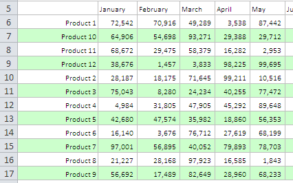
Figure 4-5: Color banding helps make your data sets easier to read.
How it works
In this macro, we are essentially using two Range object variables. One of the variables captures the scope of data we are working with, whereas the other is used to hold each individual cell as we go through the range. Then we use the For Each statement to activate or bring each cell in the target range into focus. When each row is in focus, we use the Offset property to evaluate the color index of the previous row. If the color index is white, we apply the alternate green color index.
Sub Macro41()
‘Step1: Declare your variables.
Dim MyRange As Range
Dim MyRow As Range
‘Step 2: Define the target Range.
Set MyRange = Selection
‘Step 3: Start looping through the range.
For Each MyRow In MyRange.Rows
‘Step 4: Check if the row is an even number.
If MyRow.Row Mod 2 = 0 Then
‘Step 5: Apply appropriate alternate color.
MyRow.Interior.ColorIndex = 35
Else
MyRow.Interior.ColorIndex = 2
End If
‘Step 6: Loop back to get next row.
Next MyRow
End Sub
1. We first declare two Range object variables. One, called MyRange, holds the entire target range. The other, called MyCell, holds each cell in the range as the macro enumerates through them one by one.
2. Step 2 fills the MyRange variable with the target range. In this example, we are using the selected range — the range that was selected on the spreadsheet. You can easily set the MyRange variable to a specific range such as Range(“A1:Z100”). Also, if your target range is a named range, you could simply enter its name: Range(“MyNamedRange”).
3. In this step, the macro starts through each cell in the target range, activating each cell as it goes through.
4. When a cell is activated, we determine if the current row is an even row number.
5. If the row number is indeed even, the macro uses the alternate green color index 35. If not, it uses the color index 2.
6. In Step 6, the macro loops back to get the next cell. After all of the cells in the target range are activated, the macro ends.
How to use it
The best place to store this macro is in your Personal Macro Workbook. This way, the macro is always available to you. The Personal Macro Workbook is loaded whenever you start Excel. In the VBE Project window, it will be named personal.xlb.
1. Activate the Visual Basic Editor by pressing ALT+F11.
2. Right-click personal.xlb in the Project window.
3. Choose Insert⇒Module.
4. Type or paste the code.
If you don't see personal.xlb in your project window, it doesn't exist yet. You'll have to record a macro, using Personal Macro Workbook as the destination.
To record the macro in your Personal Macro Workbook, select the Personal Macro Workbook option in the Record Macro dialog box before you start recording. This option is in the Store Macro In drop-down list. Simply record a couple of cell clicks and then stop recording. You can discard the recorded macro and replace it with this one.
Macro 42: Sort a Range on Double-Click
When you distribute your Excel reports to your customers, it's often nice to add a few bells and whistles. One of the easier enhancements to apply is the ability to sort when a column header is double-clicked. Although this may sound complicated, it's relatively easy with this macro.
How it works
In this macro, we first find the last non-empty row (using the concepts outlined in this chapter under “Macro 40: Find and Select the First Blank Row or Column”). We then use that row number to define the target range of rows we need to sort. Using the Sort method, we sort the target rows by the column we doubled-clicked.
 Double-clicking will put Excel in Edit mode, which you can cancel by pressing Esc.
Private Sub Worksheet_BeforeDoubleClick(ByVal Target As Range, Cancel As Boolean)
‘Step 1: Declare your Variables
Dim LastRow As Long
‘Step 2: Find last non-empty row
LastRow = Cells(Rows.Count, 1).End(xlUp).Row
‘Step 3: Sort ascending on double-clicked column
Rows(“6:” & LastRow).Sort _
Key1:=Cells(6, ActiveCell.Column), _
Order1:=xlAscending
End Sub
1. We first declare a Long Integer variable called LastRow to hold the row number of the last non-empty row.
2. In Step 2, we capture the last non-empty row by starting at the very last row in the worksheet and using the End property to jump up to the first non-empty cell (equivalent of going to cell A1048576 and pressing Ctrl+Shift+Up Arrow on the keyboard).
Note that you need to change the column number in this cell to one that is appropriate for your data set. That is to say, if your table starts on Column J, you would need to change the statement in Step 2 to Cells(Rows.Count, 10).End(xlUp).Row because column J is the tenth column in the worksheet.
3. In this step, we define the total row range for our data. Keep in mind that the range of rows has to start with the first row of data (excluding headers) and end with the last non-empty row. In this case, our data set starts on row 6. So we use the Sort method on Rows(“6:” & LastRow). The Key argument here tells Excel which range to sort on.
Again, you will want to ensure the range you use here starts with the first row of data (excluding the headers).
How to use it
To implement this macro, you need to copy and paste it into the Worksheet_BeforeDoubleClick event code window. Placing the macro there allows it to run each time you double-click on the sheet.
1. Activate the Visual Basic Editor by pressing ALT+F11.
2. In the Project window, find your project/workbook name and click the plus sign next to it in order to see all the sheets.
3. Click on the sheet from which you want to trigger the code.
4. Select the BeforeDoubleClick event from the Event drop-down list (see Figure 4-6).
5. Type or paste the code.

Figure 4-6: Type or paste your code in the Worksheet BeforeDoubleClick event code window.
Macro 43: Limit Range Movement to a Particular Area
Excel gives you the ability to limit the range of cells that a user can scroll through. The macro we demonstrate here is something you can easily implement today.
How it works
Excel's ScrollArea property allows you to set the scroll area for a particular worksheet. For instance, this statement sets the scroll area on Sheet1 so the user cannot activate any cells outside of A1:M17.
Sheets(“Sheet1”).ScrollArea = “A1:M17”
Because this setting is not saved with a workbook, you'll have to reset it each time the workbook is opened. You can accomplish this by implementing this statement in the Workbook_Open event:
Private Sub Worksheet_Open()
Sheets(“Sheet1”).ScrollArea = “A1:M17”End Sub
If for some reason you need to clear the scroll area limits, you can remove the restriction with this statement:
ActiveSheet.ScrollArea = “”
How to use it
To implement this macro, you need to copy and paste it into the Workbook_Open event code window. Placing the macro here allows it to run each time the workbook opens.
1. Activate the Visual Basic Editor by pressing ALT+F11.
2. In the Project window, find your project/workbook name and click the plus sign next to it in order to see all the sheets.
3. Click ThisWorkbook.
4. Select the Open event in the Event drop-down list (see Figure 4-7).
5. Type or paste the code.
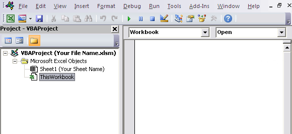
Figure 4-7: Type or paste your code in the Workbook Open event code window.
Macro 44: Dynamically Set the Print Area of a Worksheet
In certain situations, you may find yourself constantly adding data to your spreadsheets. When you do, you may have to constantly resize the print area of the worksheet to encapsulate any new data that you've added. Why keep doing this manually when you can implement a macro to dynamically adjust the print area to capture any new data you've added?
How it works
In this simple macro, we use the PrintArea property to define the range of cells that will be included when printing. As you can see, we are simply feeding the PrintArea property with the address of the UsedRange property. The UsedRange property gives us a range that encompasses the cells that have been used to enter data.
To keep this dynamic, we implement the code in the worksheet's Change event:
Private Sub Worksheet_Change(ByVal Target As Range)
ActiveSheet.PageSetup.PrintArea = ActiveSheet.UsedRange.Address
End Sub
How to use it
To implement this macro, you need to copy and paste it into the Worksheet_Change event code window. Placing the macro here allows it to run each time you double-click on the sheet.
1. Activate the Visual Basic Editor by pressing ALT+F11.
2. In the Project window, find your project/workbook name and click the plus sign next to it in order to see all the sheets.
3. Click on the sheet in which you want to trigger the code.
4. Select the Change event from the Event drop-down list (see Figure 4-8).
5. Type or paste the code.
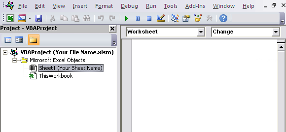
Figure 4-8: Type or paste your code in the Worksheet_Change event code window.