
Flying is so much a part of our lives that it is hard to remember that the ability to fly a heavier-than-air vehicle is barely more than a century old. The Wright brothers (Figure 4-1) succeeded where many others failed largely because of their extremely systematic approach to the problems of flight, and their recognition that the biggest problem to overcome was the control of their craft.
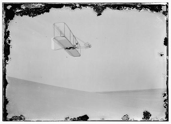
Figure 4-1. Wilbur Wright gliding to the right, attributed to either Orville or Wilbur Wright, 1902. Original on a glass negative, from the Library of Congress’ collection. Image in the public domain in the United States because of its publication before January 1, 1923. Retrieved from www.loc.gov/pictures/resource/ppprs.00604/
![]() Tip Orville and Wilbur Wright’s pragmatic, low-budget approach will be very familiar to today’s makers. David McCollough’s The Wright Brothers (Simon and Schuster, 2015) explores their approach, which could give you some ideas on the type of experiments you might want to do. Or you might just find it inspiring to see how two people with limited resources solved problems that defeated large, well-funded traditional institutions.
Tip Orville and Wilbur Wright’s pragmatic, low-budget approach will be very familiar to today’s makers. David McCollough’s The Wright Brothers (Simon and Schuster, 2015) explores their approach, which could give you some ideas on the type of experiments you might want to do. Or you might just find it inspiring to see how two people with limited resources solved problems that defeated large, well-funded traditional institutions.
A critical part of an airplane’s design is its wings. The cross-section of a wing is called an airfoil (or aerofoil, if you hail from a place that speaks British English). A modern airplane also usually has parts of the wing that move to help control the airplane, making the wing a pretty complex robotic device, not to mention the rest of the plane.
The design of a modern airline wing is a complex undertaking, occupying huge teams of people for years. However, we can get a lot of insight by looking back to a time when things were simpler and a lot more experimentally based than they are now.
This chapter looks at some historic airfoils and gives you an opportunity to 3D print them. The intent here is not to make something fly-able as much as to make something that will be a good base for experiments in a classroom or for a science fair project. If you are an aviation history buff, you will be able to create wings of some World War II–era airplanes.
![]() Note The math behind these models is more sophisticated than that behind other models in this book. In one place a basic calculus idea is used; if you have not yet had calculus, we try to explain what is going on in words, but generally speaking you can just skip that part and use the models without really understanding the math entirely. We use pseudocode for most of the equations—a mix of normal algebra symbols, but with * to show multiplication and some variables that in textbooks will just be single letters or a single letter with a subscript spelled out here instead.
Note The math behind these models is more sophisticated than that behind other models in this book. In one place a basic calculus idea is used; if you have not yet had calculus, we try to explain what is going on in words, but generally speaking you can just skip that part and use the models without really understanding the math entirely. We use pseudocode for most of the equations—a mix of normal algebra symbols, but with * to show multiplication and some variables that in textbooks will just be single letters or a single letter with a subscript spelled out here instead.
How Airfoils Work
In the Wright brothers’ day (around 1903) and for some time thereafter, airplane wings were made of fabric and strategic wood stiffeners. Every plane was an experiment, and each wing was laid up and tweaked individually. By the 1930s, engineers started to want to have some standards to work with, and our models will use some basic standards that were first defined about that time: the NACA airfoils.
Flight Forces: Lift, Drag, Gravity, and Thrust
How airplanes fly is complicated in detail. However, we can simplify it down to some basics here. Four forces are acting on an airplane. First is gravity pulling downward. Next there’s thrust (the plane’s engines) pushing it through the air. Then pushing the plane up is lift, and slowing it down (acting against the thrust) is drag. Lift and drag are closely related and affected strongly by the geometry of the aircraft.
When a plane is airborne (Figure 4-2) in stable flight, these four forces are in balance and the airplane moves ahead at a constant speed. If thrust is greater than drag, the aircraft accelerates; if there is more lift than gravity, the plane can climb. The wings have a cross-section (the airfoil) which is usually not symmetrical. In most airfoils, the top is curved more than the bottom. This makes air on top move faster and be at a lower pressure than air forced across the bottom, since air moving faster is less dense than air moving slower. This is not quite the whole story, though.
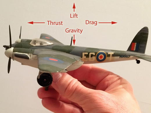
Figure 4-2. Forces on an aircraft, shown on a model of a World War II British Royal Air Force fighter-bomber, the deHavilland Mosquito—one of the last bombers made of wood. (Model courtesy of Stephen Unwin.)
You will also notice that wings tend to be rounded at the front (the leading edge) and pointy at the back (the trailing edge). A pointy edge means that air cannot circulate around the wing and get up into the lower pressure area above; instead, the flow around the wing throws off big vortices (swirling masses of air) that otherwise would have wanted to curl up around the wing. This is called the Kutta Condition (www.grc.nasa.gov/www/K-12/airplane/lifteq.html).
The equation for lift is Lift = 0.5 * CL * ρ * v2 * A. Here’s what the symbols mean: the density of the air in which the aircraft is traveling is the Greek letter ρ (pronounced “rho”). v2 is the square of its velocity. A is the planform area of the wing (the area of the wing as seen from above). Finally, CL is a fudge factor called the lift coefficient (https://en.wikipedia.org/wiki/Lift_coefficient) which depends on the geometry of the wing and some factors about how the plane is flying, and is usually measured experimentally.
![]() Example At sea level, if a plane is going 100 miles an hour at takeoff (about 45 m/s), air density is 1.23 kg/m3, wing area is around 100 square meters, and lift coefficient is about 1, then we get about 124 kN, or 27,000 pounds-force, of lift. The lift coefficient usually varies a lot with the angle the plane’s nose is holding relative to the horizontal, called angle of attack (more on this in a later section).
Example At sea level, if a plane is going 100 miles an hour at takeoff (about 45 m/s), air density is 1.23 kg/m3, wing area is around 100 square meters, and lift coefficient is about 1, then we get about 124 kN, or 27,000 pounds-force, of lift. The lift coefficient usually varies a lot with the angle the plane’s nose is holding relative to the horizontal, called angle of attack (more on this in a later section).
Drag is the resistive force that holds back the airplane as it flies through the air. Drag is the same equation as lift, with a different coefficient (CD instead of CL). There is a list of of some values of drag coefficient for different shapes at https://en.wikipedia.org/wiki/Drag_coefficient. So that your plane can fly a long way on a reasonable amount of fuel, you need to have a big lift coefficient and a small drag coefficient. In practice they are closely related, and airplane designers have to work to get one as big as possible and push the other down. The ratio of lift to drag is a common performance metric for aircraft.
Chord, Camber, and Thickness
The Wright brothers built on work by others, notably George Cayley (1773–1857), who has been generally credited with defining some of the key features of working wings. If you look at a bird, you see that the wing has a lot of structure and is not just a flat plate tilted to the wind somehow.
Over time, people have developed conventions for ways to describe a wing. There are a lot of subtle ones, but we will just talk about a few of the easiest-to-understand ones in this chapter (and give you some suggestions about where to learn more at the end). Figure 4-3 is a diagram of the parts of an airfoil. The straight-line distance from the leading edge to the trailing one is called the chord.
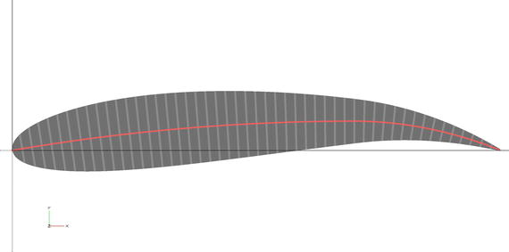
Figure 4-3. Airfoil (NACA 6715). The red middle line is the camber line
Wings usually are curved a bit from front to back. The line that describes this curve is called the camber line. The thickness of the airfoil is how thick it is, typically measured at the point of maximum thickness or maximum camber.
Camber, thickness, and the location of maximum camber and maximum thickness are typically given relative to the chord (as a percentage of, or in tenths of, the chord.) Or to put it another way, the numbers are figured out for a chord that is 1 unit long, and you would then scale everything accordingly. In Figure 4-3, the chord is the straight (x-axis) line distance from leading to trailing edge. The red line right through the middle is the camber line. The short grey lines from the upper to the lower surface, perpendicular to the camber line, represent the thickness of the airfoil at any given point along the camber line.
![]() Note If you have had some calculus, you can read about the Kutta-Jukowski theorem (https://en.wikipedia.org/wiki/Kutta%E2%80%93Joukowski_theorem) to understand a bit better how the phenomenon called circulation creates lift on a wing. For our purposes here, it is enough to think about a wing throwing off air partially downward to create a lift force. A big, heavy aircraft has so much energy in the vortices it leaves in its wake that aircraft have to be separated by miles to allow the vortices to dissipate. There is also a good interactive discussion of all these topics in the NASA Glenn Beginner’s Guide to Aeronautics at www.grc.nasa.gov/ www/K-12/airplane/.
Note If you have had some calculus, you can read about the Kutta-Jukowski theorem (https://en.wikipedia.org/wiki/Kutta%E2%80%93Joukowski_theorem) to understand a bit better how the phenomenon called circulation creates lift on a wing. For our purposes here, it is enough to think about a wing throwing off air partially downward to create a lift force. A big, heavy aircraft has so much energy in the vortices it leaves in its wake that aircraft have to be separated by miles to allow the vortices to dissipate. There is also a good interactive discussion of all these topics in the NASA Glenn Beginner’s Guide to Aeronautics at www.grc.nasa.gov/ www/K-12/airplane/.
NACA Airfoils
After World War I ended, it was clear that some design rules about how to make a good wing were needed to take the next steps in aviation. The Aerodynamic Research Institute of Göttingen, in Germany, did one of the first systematic studies of wings, called Joukowsky Profiles, from 1923–1927.
Meanwhile, in the United States, the National Advisory Committee on Aeronautics (NACA) was formed in 1915 to coordinate aeronautics research. (In 1958, it was closed down and merged into NASA.) In 1932, according to a NASA history chronology (www.hq.nasa.gov/office/pao/History/Timeline/1930-34.html), a first set of NACA airfoils was published, which are thought to have been inspired to some degree by the German ones. Over the next few years wind tunnel tests (see sidebar) were performed on some of the more promising airfoils. More sets were developed over time and have since been published and put in the public domain.
Fundamentally, the NACA profiles gave an equation for the camber line relative to the chord and another one for how thick the airfoil should be at any point along the chord. These equations were experimentally developed, and a lot of the theory about why these were good airfoils came much later.
WIND TUNNELS
A wind tunnel is, in its most basic form, a box with a fan on one end and an opening on the other which allows an engineer to flow air over a model in a controlled way. A model is held on a sting (which can just be a stick), and the different forces on it are measured somehow. Or sometimes a tunnel will just have a way to mix a little smoke in with the flow so that users can watch what the smoke does when it interacts with the vehicle design. The wing models we show you how to make in this chapter are designed to allow you to explore how a wing works, or just to appreciate some early wing designs as works of engineering art.
In the “Science Fair Projects” suggestions at the end of this chapter, we have some links to project sites that talk about how you might build a small student wind tunnel for students to learn about basic aerodynamics.
The NACA Four-Digit Series
The first set of NACA airfoil profiles are called the four-digit profiles, because each profile is defined with four numbers, like NACA 2412 (a classic airfoil that is still used in some general-aviation aircraft today). The digits of the airfoil NACA abcd are interpreted as follows:
First digit (a): the maximum distance the camber profile goes above the chord (in what we are calling the y direction), as a percentage of the chord. You multiply this number by 0.01 times the chord to get the actual distance. If the chord was 1 meter long, for a 2412 airfoil the maximum camber distance from the chord would be 2 times 0.01 times 1 meter, or 0.02 meters (2 cm).
Second digit (b): the location along the chord, in what we are calling the x direction, starting at the leading edge where the maximum camber occurs as a tenth (not a percentage) of the chord. You multiply this number by 0.1 times the chord to get the location. For our 1 meter chord wing and a 2412 airfoil, this means this location would be 0.4 times 1 meter from the leading edge, or 40 cm from the leading edge.
Third and fourth digit (cd): The maximum thickness above and below the chord, as a percentage of the chord. There is an equation to plug this number into to get the thickness at any given point along the chord. The maximum thickness in our example would be 12% of 1 meter, or 120 cm on either side of the camber line, and is measured perpendicular to the camber line (see Figure 4-3).
To summarize our example (NACA 2412, a = 2, b = 4, cd = 12) has a thickness that is 12% of the chord; has a camber that is 2% of the chord at its maximum point; and that maximum happens 40% of the chord away from the leading edge of the wing (Figure 4-4).
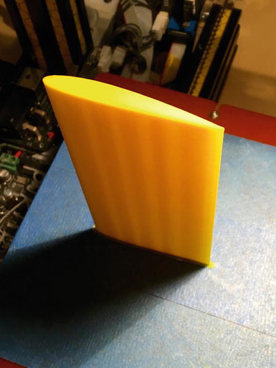
Figure 4-4. NACA 2412 model, as created by the model in Listing 4-1
In the section later in this chapter, “Thinking About These Models: Learning Like a Maker,” we talk about how we went all the way back to a 1935 report to wade through inconsistent naming conventions for these parameters (some people use mpxx, some pmxx, some other things). We also shuffled the equations around a little to make them work better with OpenSCAD. Here we walk through them from first principles. If you look them up elsewhere, you will find the equations a little different. We found in many places online that they were simply wrong, so use online sources like people’s class notes or Wikipedia with care.
Later on, other NACA airfoil series were developed that had more complicated profiles. The early ones were intended to be rules of thumb that could be used as guides in the pre-computer days. Now wings are very complicated things, but you can learn a lot by going back to those simpler times and re-creating some of these early experiments.
NACA Four-Digit Profiles in OpenSCAD
The NACA four-digit airfoil model is made up of two curves: a camber line that defines the curve of the centerline of the airfoil, and a function that defines how thick the airfoil is on either side of this curve. Confusingly, camber is the distance from the chord to the camber line.
The Camber Line
The camber line is derived from two parabolas, each of which has a maximum at the point of maximum camber (Figure 4-5). Everything in what follows is computed for a wing with a unit chord; everything will then be scaled to that proportionately. The x axis is along the chord. The equations of the parabolas for the camber line are as follows:
For x less than or equal to b:
ycamber = (a/b2)(2bx – x2)
For x greater than or equal to b:
ycamber = ( (a/(1 – b)2)(1 – 2b + 2bx – x2).
Notice that when x = b, then either one results in ycamber = a.
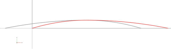
Figure 4-5. The two parabolas making up the camber line. The red line is the halves of the two parabolas that are used to create the camber line, while the grey line is the unused portion of each parabola. The maximum is at x = b, y = a, if the chord is equal to 1
The Thickness Equation
The camber line is just an abstract, infinitely thin line. The thickness equation tells us how much the airfoil extends at any point on either side perpendicular to the camber line. The equation for thickness that follows is what you might think of as half the thickness of the wing; it is how far away the wing surface is from the camber line, toward the upper or lower surface.
Some airfoils have different top and bottom thickness profiles, which complicates deriving the camber line. The NACA four-digit ones use the same equation for both, and thus the camber line could be written as a (relatively) simple equation as well. For the four-digit airfoils the maximum thickness as a percentage of the chord is the last two digits (cd) of the NACA airfoil:
thickness(x) = (cd/20)(0.2969 * sqrt(x) – 0.1260 * x – 0.3516 * x2 + 0.2843 * x3 – 0.1015 * x4).
However, this is the thickness perpendicular to the camber line, and assuming that the chord is 1 unit long. To get it in terms of x and y, we want to figure out what direction is perpendicular to the line. An easy way to do this (if you have had calculus) is to take the derivative (the slope) of the tangent line. (See the “Learning Like a Maker” section for references for these equations, which were in somewhat different form in the 1935 reference.)
The equations of the slope of the camber line, d(ycamber)/dx, are as follows:
For x less than or equal to b:
d(ycamber)/dx = (2a/b2)(b – x)
For x greater than or equal to b:
d(ycamber)/dx = ((2a/(1 – b)2) * (b – x)
If you have not had calculus yet, what we are doing here is picking a point on the camber line and figuring out what the slope of a line that is tangent to the curve of the camber line is at that point. (Isaac Newton needed to solve similar problems and invented calculus to do it.) Then we use that tangent line to figure out how to get the thickness (which is defined in a direction perpendicular to the camber line) at that same point. If you like, you can think if it as transforming the thickness into a coordinate system that is sliding along the camber line.
To do that coordinate transformation, we first define an angle theta to be the angle whose tangent is d(ycamber)/dx. Then the equations we get for the airfoil surface (camber line plus thickness component perpendicular) are as follows:
theta = arctan(((2a/(1 – b)2) * (b – x))
x(lower) = x + sin(theta) * thickness(x)
y(lower) = ycamber – cos(theta) * thickness(x)
x(upper) = x – sin(theta) * thickness(x)
y(upper) = ycamber + cos(theta) * thickness(x)
In our OpenSCAD model (Listing 4-1), we do not actually calculate the x and y coordinates of each point on the upper and lower surface. Instead, we just use OpenSCAD’s built-in rotate() function to rotate a shape centered on the camber line so that its minimum and maximum points fall on the upper and lower surface lines. Ideally, these shapes would simply be line segments with a length determined by the thickness function. You can see these ideal lines in the grey lines perpendicular to the camber line in Figure 4-3.
However, because OpenSCAD does not have a concept of lines with no area or volume, we simulated these lines with very thin rhomboids (Figure 4-6), which become infinitely thin where they meet the top and bottom surface lines. We created these using a "circle" with four sides with circle($fn = 4) and scaling this "square circle" in the x and y directions. circle($fn = 4) is a shorter way of producing the same thing we would get by creating a square measuring two units corner-to-corner and rotating it, which you would do in OpenSCAD with rotate(45) square(sqrt(2), center = true). Note that the rhomboids in Figure 4-6 are thicker and fewer than the ones actually used to make the wing profile.
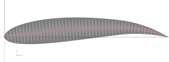
Figure 4-6. The geometry of rhombuses which are bisected by the tangent to the camber line. Airfoil is NACA 6715
We then use the convex hull fuction hull() to fill in the space between each of these rhomboids in order to create the profile of our wing. All this results, in our first pass, in an airfoil that has a NACA four-digit profile (and is a flat wing—not swept back. Listing 4-1 gives the model for this basic wing, which also has the capability of using sweep and taper (defined in the next section).
Other Aerodynamic Parameters
Modern wings are rarely straight across with the same airfoil cross-section all the way along the wing. Here are some other things that affect how a wing works (and how it appears). The models in this chapter can handle the following two variables, in addition to their airfoil profiles:
Sweep: If you look at a modern jet aircraft, the wings sweep back at an angle, rather than having a leading edge that is straight across. This became important once jet aircraft were introduced and planes were going very fast. Jet aircraft now cruise near the speed of sound; right at the speed of sound, a plane creates shock waves that are experienced on the ground as sonic booms and on the plane in a variety of ways. A swept wing allows the plane to fly closer to the speed of sound than it would if it had a straight wing.
Taper: Tapered wings get thinner as they get farther from the fuselage (but maintain the same airfoil cross-section, as implemented here). The model in this chapter requires that swept wings be tapered. You might want to play with the two variables and see how the models change.
Angle of attack: Airplanes tilt up steeply as they are climbing away from the ground both because they are trying to get away from the ground quickly, but also because (to a point) a higher angle relative to the flow generates more lift (see previous section). The angle of the chord line to the horizontal direction of flight is called angle of attack. Typically drag also increases with angle of attack, so this is one of the many things to trade off in aircraft design. (We talk about this when we get to the model in Listing 4-2.)
The current model does not support some other wing design features such as dihedral. If the wings bend upward from the root to the tip, we say that the wings “have dihedral” or that the dihedral angle is greater than zero. The angle is defined from a line perpendicular to the chord. Dihedral has implications for aircraft stability.
Classic Airplanes Using NACA Airfoils
The NACA models were developed a little before World War II. All the airplanes flying in those days were what we would now consider to be low speed. The NACA airfoils were used heavily in World War II airplanes on all sides of the conflict. The Incomplete Guide to Airfoil Usage, at http://m-selig.ae.illinois.edu/ads/aircraft.html, has many examples. The same group’s home page at http://m-selig.ae.illinois.edu/ads.html has links to other aircraft modeling tools and sites.
You will see on the site that many airplanes used one airfoil design at the root of the wing (where it connects to the fuselage) and another at the tip. For example, according to the Incomplete Guide, the workhorse early prop-driven airliner, the DC-3, used NACA 2215 at the root and 4412 at the tip. Many Cessnas have used the common 2412 airfoil.
If you are a fan of British aviation history, the Incomplete Guide notes that the World War II Supermarine Spitfire used two NACA profiles in its wings (2213 at its root, 2209.4 at its tip, where the decimal point means 09.4% maximum thickness). The Spitfire was the classic Royal Air Force (RAF) interceptor during the Battle of Britain. Figure 4-7 is a kit created in the 1960s by the child of a WWII RAF officer.
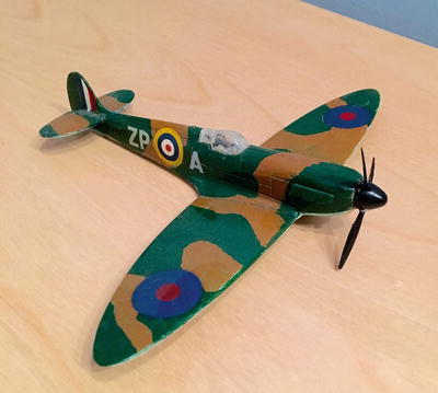
Figure 4-7. WWII Supermarine Spitfire model (courtesy of Stephen Unwin)
We have not created the capability to replicate the exact details of any given actual wing (the model requires that you have one NACA profile for the whole wing). Rather, our intent is that you can pretend to be the designer of an historic vehicle and play around with changing its basic profile. In short, how might you have designed an airplane during World War II? Or for a low-speed application today? Or to understand why different birds have the wing shapes they do? It is all yours to explore.
Using the 3D-Printed Airfoil Models
The basic OpenSCAD model in Listing 4-1 will print one wing. If it is not symmetric (if it is swept, for example) you will need to use MatterControl (see Appendix A) or your equivalent 3D-printer software to mirror the wing if you want two to make yourself a whole airplane to study.
If you want to study the aerodynamics of a wing, Listing 4-2 creates two wings and a test stand (called a sting) that will allow it to stand in a wind tunnel or other place that you make observations or measurements. We are also including a version of the model (Listing 4-2) that includes a sting with a ratched mechanism that allows you to vary the angle of attack in a range that you set. The next section talks about simple ways to measure lift.
![]() Caution The sting model is intended to allow for some basic classroom experiments in changing angle of attack and measuring the resulting lift. It is not very aerodynamic and introduces a lot of drag, and we have not talked about measuring drag. If you are interested in measuring anything other than lift, we suggest going back to the OpenSCAD model and adding your own attachments for more sophisticated instruments. Since this is an open source model, see Appendix A for links to add your creation, if you would like, to the community (and to see what others might have added since the book was published).
Caution The sting model is intended to allow for some basic classroom experiments in changing angle of attack and measuring the resulting lift. It is not very aerodynamic and introduces a lot of drag, and we have not talked about measuring drag. If you are interested in measuring anything other than lift, we suggest going back to the OpenSCAD model and adding your own attachments for more sophisticated instruments. Since this is an open source model, see Appendix A for links to add your creation, if you would like, to the community (and to see what others might have added since the book was published).
Measuring Lift
We saw earlier in this chapter that Lift = 0.5 * CL * ρ * v2 * A, where ρ is the density of air (about 1.23 kg per cubic meter). The lift coefficient, CL, will vary with angle of attack but will be around 1 or 2 (see the 1935 report referenced in the “Thinking Like a Maker” section that follows). The model in Listing 4-2 creates a pair of wings, a sting, and a stand that you can weigh down (with coins, for instance).
You also need to attach the two wings to each other, say with blue tape (as we show here) or by gluing. The base will let you set an angle of attack range. In the example, it goes from 0 to 25 degrees in 5-degree increments.
Then, if you put the whole thing on a sensitive scale (like an electronic postal scale, or a scale you have in your school lab) you will get a setup that looks like the one in Figure 4-8. This model used a NACA 2412 airfoil with a chord 60 mm long, a taper of 2, and a wing length of 80 mm (times 2, for the pair).
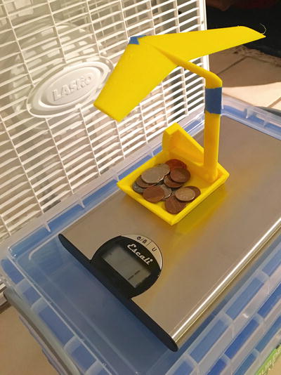
Figure 4-8. Using the output of the model in Listing 4-2 to measure lift
![]() Tip To get the area of a tapered wing, you have to figure out the area of a trapezoid with the sides being the root chord and tip chord. To do that, you average the two chords and multiply by the wingspan. In the case of our example, we would get
Tip To get the area of a tapered wing, you have to figure out the area of a trapezoid with the sides being the root chord and tip chord. To do that, you average the two chords and multiply by the wingspan. In the case of our example, we would get
Area = 0.5 * (tip chord + root chord) * wingspan. In our example here,
Area = 0.5 * (60 mm + 30 mm) * 80 mm * 2 wings = 0.0072 square meters.
For more planforms, see www.grc.nasa.gov/www/k-12/airplane/area.html.
If the airflow is about 9 miles per hour (about 4 meters per second), then the lift should be around 0.5 * 1 * 1.23 * 4 * 4 * 0.0072 = 0.0709 Newtons, or has the ability to lift about 7 grams if you prefer to think that way, for a drag coefficient equal to 1.
![]() Tip For more ideas on simple ways to measure lift, see the slides “Wind Tunnel Experiments for Grades 8–12, ” available at www.grc.nasa.gov/WWW/k-12/airplane/topics.htm.
Tip For more ideas on simple ways to measure lift, see the slides “Wind Tunnel Experiments for Grades 8–12, ” available at www.grc.nasa.gov/WWW/k-12/airplane/topics.htm.
If you zero out the scale when the fan is off, you should get a negative number for the weight of the sting plus the airfoil when you turn it on. That number is the lift (with a fair number of sources of error). The model (Figure 4-9) allows you to play with the angle of attack, and of course you can print different profiles. You will need to find some way of measuring how fast the flow coming out of the fan is, and its direction—you can make, buy, or borrow a cup anemometer as a simple instrument (a search will reveal both plans to make and places to purchase one). You can take a small piece of string and hold it in front of the wing to see if you are in an area of the fan outflow that has smooth airflow. We guesstimated the flow out of the fan by dropping a small scrap of tissue and seeing how long it took to go a few meters, but this is really too error-prone to use closer than a factor of two or so, since the flow mixes very quickly with the ambient still air.
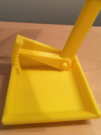
Figure 4-9. Closeup of the angle of attack ratchet on the support
In our experiment here, an angle of attack of zero gave us enough lift to raise about 10 grams; of 15 degrees, about 13; and of 25 degrees, about 8 grams. The 1935 paper seems to show that a clean 2412 wing should have a lift coefficient about 0.2 at 0 degrees angle of attack; about 1.3 at 15 degrees; and at around 25 degrees or so it should stall and drop off precipitously. Given the many variables (like the effects of the test stand and the placement in the fan’s not-particularly-even flow) this is more or less reasonable. We encourage you to work out ways to make this far more accurate!
Household fans often have dead spots. You may need to play around a bit to get good results—staying a couple feet away from the fan helps, but not too far, since the flow will be too diffuse. To do this right, you need to create a wind tunnel, the device that controls air around a test airplane; see the “Building a Student Wind Tunnel” resources at the end of the chapter.
![]() Note These models are not meant to be flying models. They will barely lift their own weight at reasonable speeds. They are meant to be sturdy enough to stand up to some experimentation and analysis, rather than being as light as possible. Your 3D printer software will give you a weight estimate for the wing (which in the case of the Listing 4-2 models will include the sting and the base).
Note These models are not meant to be flying models. They will barely lift their own weight at reasonable speeds. They are meant to be sturdy enough to stand up to some experimentation and analysis, rather than being as light as possible. Your 3D printer software will give you a weight estimate for the wing (which in the case of the Listing 4-2 models will include the sting and the base).
Printing Suggestions
These models are meant to be as easy as possible to print, given that the geometry is fairly complicated. Print them with the chord side down, as the models were designed. You should not need to use support, but you probably want to use a brim or raft so that the model sticks to the platform. For the STL output by Listing 4-2, you may need to move the pieces around to fit your platform, or print it in more than one print. You will want to make sure that you have printer settings that allow brim or raft to be removed cleanly, though, because any remaining pieces will interfere with assembly of the sting mechanism. Figure 4-10 shows how the model appeared on the 3D-printer platform.
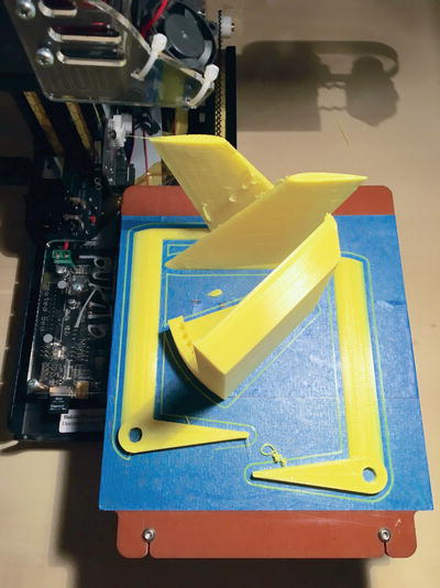
Figure 4-10. The layout of the models as printed
![]() Caution Do not scale these models in your 3D printing program; use the scaling parameters in the models in OpenSCAD and generate a new STL. There are issues of tolerances and some complex interactions that may break if you just scale without taking account of these issues.
Caution Do not scale these models in your 3D printing program; use the scaling parameters in the models in OpenSCAD and generate a new STL. There are issues of tolerances and some complex interactions that may break if you just scale without taking account of these issues.
THINKING ABOUT THESE MODELS: LEARNING LIKE A MAKER
When we started this chapter we thought we would be done in a couple of hours. We knew there were equations for the NACA airfoils, and we thought we would use techniques similar to those in we used in Chapter 1 to create the top and bottom as 3D surfaces.
No such luck.
The NACA airfoils are interesting in that they were created to make hand calculation (in the 1930s) as simple as possible, and were purely empirically based. They were also extensively cited, but inconsistently. Over time, authors seem to have lost some of the assumptions underlying the original model, or just appeared to make transcription errors. Some authors used the letter p for the first digit, and m for the second; somewhere in the 1970s this seemed to reverse. (To avoid getting a lot of letters from people who found references one way or the other, we changed here to an abcd convention.) Authors inconsistently used either the ratio of the thickness to the chord, or the dimensioned number.
We decided to go all the way back to the oldest possible description of the NACA series and to look at the physics there. Fortunately, all these old reports are available for free from the NASA Tech Reports Service (http://ntrs.nasa.gov). We started digging and discovered that the report everyone seemed to cite as a first place the airfoils were described in detail was NACA Report 460, published in 1935 by E.N. Jacobs, K.E. Ward, and R.M. Pinkerton. This report, The Characteristics of 78 Related Airfoil Sections from Tests in the Variable-Density Wind Tunnel, is an amazing period piece. Two of the advisors listed in the front matter were Charles Lindbergh and Orville Wright! Pages 4 and 5 of the report have very clear drawings that we used as the basis of the OpenSCAD model.
If you look in the back of the 1935 report (with its many hand-drawn graphs), you can see wind tunnel data that might be a good place for you to begin designing a classroom demonstration or a great science fair project.
Where to Learn More
There is a tremendous amount of information out there about airfoils; the challenge for this chapter has been to curate a set of interesting explorations that would be accessible for a wide range of student levels. In this section, we suggest some sensible bigger projects for you to take on if just informally playing with these airfoils is not enough. Another good general site on the topic, in addition to ones given so far, is http://airfoiltools.com, which has a variety of interesting calculators and plotting tools.
NASA Glenn Research Center also has an exhaustive site with many good ideas. The main index is at www.grc.nasa.gov/WWW/K-12/airplane/bgt.html, and many presentations available for teachers are indexed at www.grc.nasa.gov/WWW/K-12/airplane/topics.htm.
You can take projects about airfoils in several directions. As a first thought, you can look at it as the history of aviation and the study of the development of aviation from 1903 through the 1930s and beyond. Or you can treat this as a basic physics exercise to see how changing some of these basic parameters like camber and thickness changes the lift and drag of the wing.
Building a Student Wind Tunnel
To actually test out the wings in a quantitative way, you will need to make yourself some sort of wind tunnel. We have not tried this ourselves, but with that caveat we will note that this project seems plausible, although probably best suited for a group, rather than individual, project: www.sciencebuddies.org/science-fair-projects/wind-tunnel-toc.shtml. If you wanted to build a tunnel purely to visualize the flow around the wing (versus trying to measure lift and drag), this Instructable has a simpler build: www.instructables.com/id/DIY-Wind-Tunnel-20-Project-Paperclip/.
Visualizing Flow
To learn more about ways to visualize what the air flowing over wings is doing, try searching on “flow visualization.” There is also a classic book you might hunt down: An Album of Fluid Motion, by Milton Van Dyke (Parabolic Press, 1982), which is just an entire book of pictures of flow in various test conditions.
Scaling a Model
If you are going to seriously try to model a real system (like a bird or an airplane) with a wind tunnel model that is a lot smaller than the original, you will need to match the Reynolds number (Re) of your model and the real system to get accurate results. The Reynolds number is a ratio of the kinetic energy in a system to the effects of viscosity. Viscosity is how “sticky” a fluid is—maple syrup is pretty viscous, but air less so. (Engineers do not draw distinctions between liquids and gases here—it’s all “fluids” to us.)
High Re flow could be found in a fast-flowing water stream; low Re is exemplified by molasses coming out of a jar. The two extremes behave quite differently. The equation for Reynolds number is usually written: Re = ρ v L/μ.
Where ρ is still the density of the air (or fluid) around the wing, v is the velocity, L is a characteristic length of the thing you are testing (like the chord or the wingspan), and μ is the dynamic viscosity of the air or other fluid.
If you are modeling something big with a 1/10th scale model, to have the Reynolds number of your model be the same as the real thing you need to run your test with ten times higher velocity or ten times denser or more viscous flow (or a combination that works out to that). For air at the surface of the earth at 15 degrees Centigrade, the density and viscosity are, respectively, ρ = 1.23 kg/m3 and μ = 1.78 x 10– 5 kg/m-s; for water, ρ= 999 kg/m3; and μ = 115.4 x 10⁻⁵ kg/m-s (from A.M. Kuethe and C-Y Chow, Foundations of Aerodyamics 3rd Edition (Wiley, 1976).
Using flowing water as a test fluid is thus the same as air at the same velocity around an object about 12 times bigger. Water tunnels have been developed to exploit this, but obviously this is pretty challenging and messy.
Teacher Tips
The science of flight is usually not encountered in depth until undergraduate-level science courses, since to get very far into the analysis you really need to have some calculus. That said, the empirical study of the forces on a wing might fit well under the NGSS standards (MS-PS-2, www.nextgenscience.org/msps2-motion-stability-forces-interactions) and Energy standards (MS-PS-3, www.nextgenscience.org/msps3-energy).
That said, there are many topics that could be covered purely to build intuition. We have suggested many possible experiments in this chapter; some might lend themselves to labs at almost any level. In particular, working to refine how accurate the model is will be a good long-term project for any number of students.
Science Fair Project Ideas
A wind tunnel, even the small ones described in the “Where to Learn More” section, is probably physically too big to bring to most science fairs. However, if a school or class builds one, testing a series of models to find their lift and drag might be an interesting project.
You might also see which airfoils could approximate a bird’s wing and try to think about how to model how well a bird “should” fly.
But if all that sounds too complicated, you can always create a few airfoils and just test them qualitatively in front of a box fan. Consider ways to make simple ways to measure lift and drag using weights to balance the forces. Or perhaps create some wing cross-sections to see which ones might match various bird wings. Or, for that matter, you can just drag them through a bathtub and see if you can feel any difference.
Summary
In this chapter, we talked about airfoils and offered a simple model that was used in the 1930s to learn more about how wings work. We discovered that the mathematics behind flight are complex, but that there are some simplified models, like the NACA airfoils, that can help build intuition (and that are still in use today). We looked at how we might use those models today to learn about flight, and perhaps to help understand birds or other flying creatures.