Appendix B
Measure and integration
The axiomatic approach to probability by Andrey Kolmogorov (1903–1987) makes essential use of the measure theory. In this appendix we review the aspects of the theory that are relevant to us. We do not prove everything and refer the interested reader for proofs and further study to one of the many volumes on this now classic subject, see e.g. [7, 27].
B.1 Measures
B.1.1 Basic properties
Here Ω shall denote a generic set. For a generic subset E of Ω, Ec := Ω E denotes the complement of E in Ω and ![]() (Ω) denotes the family of all subsets of Ω. A family
(Ω) denotes the family of all subsets of Ω. A family ![]() of subsets of Ω is then a subset of
of subsets of Ω is then a subset of ![]() (Ω),
(Ω), ![]() ⊂
⊂ ![]() (Ω). We say that a family
(Ω). We say that a family ![]() ⊂
⊂ ![]() (Ω) of subsets of a set Ω is an algebra if
(Ω) of subsets of a set Ω is an algebra if ![]() , Ω
, Ω ![]()
![]() and E ∪ F, E ∩ F and Ec
and E ∪ F, E ∩ F and Ec ![]()
![]() whenever E, F
whenever E, F ![]()
![]() .
.
Definition B.1 We say that ![]() is a σ-algebra if
is a σ-algebra if ![]() is an algebra and for every sequence of subsets
is an algebra and for every sequence of subsets ![]() we also have ∪k Ek and ∩k Fk
we also have ∪k Ek and ∩k Fk ![]()
![]() .
.
In other words, if we operate on sets of a σ-algebra with differences, countable unions or intersections, we get sets of the same σ-algebra: we also say that a σ-algebra is closed with respect to differences, countable unions and intersections.
Let ![]() ⊂
⊂ ![]() (Ω) be a family of subsets of Ω. It is readily seen that the class
(Ω) be a family of subsets of Ω. It is readily seen that the class
![]()
is again a σ-algebra, hence the smallest σ-algebra containing ![]() . We say that
. We say that ![]() is the σ-algebra generated by
is the σ-algebra generated by ![]() .
.
Definition B.2 The smallest σ-algebra ![]() containing the open sets of
containing the open sets of ![]() is called the σ-algebra of Borel sets.
is called the σ-algebra of Borel sets.
Definition B.3 A measure on Ω is a couple (![]() ,
, ![]() ) of a σ-algebra
) of a σ-algebra ![]() ⊂
⊂ ![]() (Ω) and of a map
(Ω) and of a map ![]() with the following properties:
with the following properties:
(i) ![]() (
(![]() ) = 0.
) = 0.
(ii) (Monotonicity) If A, B ![]()
![]() with A ⊂ B, then
with A ⊂ B, then ![]() (A) ≤
(A) ≤ ![]() (B).
(B).
(iii) (σ-additivity) For any disjoint sequence ![]() we have
we have
![]()
Obviously (iii) reduces to finite additivity for pairwise disjoint subsets if ![]() is finite. When
is finite. When ![]() is infinite, the infinite sum on the right-hand side is understood as the sum of a series of non-negative terms. From Definition B.3 we easily get the following.
is infinite, the infinite sum on the right-hand side is understood as the sum of a series of non-negative terms. From Definition B.3 we easily get the following.
Proposition B.4 Let (![]() ,
, ![]() ) be a measure on Ω. We have:
) be a measure on Ω. We have:
(i) If A ![]()
![]() , then 0 ≤
, then 0 ≤ ![]() (A).
(A).
(ii) If A, B ![]()
![]() with A ⊂ B, then
with A ⊂ B, then ![]() (B A) +
(B A) + ![]() (A) =
(A) = ![]() (B).
(B).
(iii) If A, B ![]()
![]() then
then ![]() (A ∪ B) +
(A ∪ B) + ![]() (A ∩ B) =
(A ∩ B) = ![]() (A) +
(A) + ![]() (B).
(B).
(iv) If A, B ![]()
![]() then
then ![]() (A ∪ B) ≤
(A ∪ B) ≤ ![]() (A) +
(A) + ![]() (B).
(B).
(v) (σ-subadditivity) For any sequence ![]() we have
we have
(vi) (Disintegration formula) If ![]() is a partition of Ω, then for every A ⊂ Ω,
is a partition of Ω, then for every A ⊂ Ω,
(vii) (Continuity)
(a) If ![]() with Ei ⊂ Ei+1 ∀i, then
with Ei ⊂ Ei+1 ∀i, then ![]() and
and
(b) Let ![]() be such that Ei ⊃ Ei+1 ∀i. Then
be such that Ei ⊃ Ei+1 ∀i. Then ![]() and more-over, if
and more-over, if ![]() (E1) < +∞, then
(E1) < +∞, then
Proof. (i)–(vi) follow trivially from the definition of measure. Let us prove claim (a) of (vii). Since ![]() (Ek) ≤
(Ek) ≤ ![]() (∪k Ek) for every k, the claim is trivial if for some k
(∪k Ek) for every k, the claim is trivial if for some k ![]() (Ek) = +∞. We may therefore assume
(Ek) = +∞. We may therefore assume ![]() (Ek) < ∞ for all k. We set E := ∪k Ek and decompose E as
(Ek) < ∞ for all k. We set E := ∪k Ek and decompose E as
![]()
The sets E1 and Ek Ek−1, k ≥ 1, are of course in ![]() and pairwise disjoint. Because of the σ-additivity of
and pairwise disjoint. Because of the σ-additivity of ![]() we then have
we then have

Claim (b) of (vii) easily follows. In fact, since ![]() (E1) < +∞ and Ek ⊂ E1, we have
(E1) < +∞ and Ek ⊂ E1, we have ![]() (Ek) =
(Ek) = ![]() (E1) −
(E1) − ![]() (E1 Ek) for all k. Since
(E1 Ek) for all k. Since ![]() is an increasing sequence of sets, we deduce from (a) that
is an increasing sequence of sets, we deduce from (a) that

Let (![]() ,
, ![]() ) be a measure on Ω. We say that N ⊂ Ω is
) be a measure on Ω. We say that N ⊂ Ω is ![]() -negligible, or simply a null set, if there exists E
-negligible, or simply a null set, if there exists E ![]()
![]() such that N ⊂ E and
such that N ⊂ E and ![]() (E) = 0. Let
(E) = 0. Let ![]() be the collection of all the subsets of Ω of the form F = E ∪ N where E
be the collection of all the subsets of Ω of the form F = E ∪ N where E ![]()
![]() and N is
and N is ![]() -negligible. It is easy to check that
-negligible. It is easy to check that ![]() is a σ-algebra which is called the
is a σ-algebra which is called the ![]() -completion of
-completion of ![]() . Moreover, setting
. Moreover, setting ![]() (F) :=
(F) := ![]() (E) if F = E ∪ N
(E) if F = E ∪ N ![]()
![]() , then (
, then (![]() ,
, ![]() ) is also a measure on Ω called the
) is also a measure on Ω called the ![]() -completion of (
-completion of (![]() ,
, ![]() ). It is often customary to consider measures as
). It is often customary to consider measures as ![]() -complete measures.
-complete measures.
B.1.2 Construction of measures
B.1.2.1 Uniqueness
Let (![]() ,
, ![]() ) be a measure on Ω. The σ-additivity property of
) be a measure on Ω. The σ-additivity property of ![]() suggests that the values of
suggests that the values of ![]() on
on ![]() are in fact determined by the values of
are in fact determined by the values of ![]() on a restricted class of subsets of
on a restricted class of subsets of ![]() .
.
Definition B.5 A family ![]() ⊂
⊂ ![]() (Ω) of subsets of Ω is said to be closed under finite intersections if A, B
(Ω) of subsets of Ω is said to be closed under finite intersections if A, B ![]()
![]() implies A ∩ B
implies A ∩ B ![]()
![]() .
.
A set function ![]() is σ-finite if there exists a sequence
is σ-finite if there exists a sequence ![]() such that Ω = ∪k Ik and α(Ik) < ∞ ∀k.
such that Ω = ∪k Ik and α(Ik) < ∞ ∀k.
We have the following coincidence criterion. A proof can be found in, e.g. [7].
Theorem B.6 (Coincidence criterion) Let ![]() and
and ![]() be two measures on Ω and let
be two measures on Ω and let ![]() be a family that is closed under finite intersections. Assume that
be a family that is closed under finite intersections. Assume that ![]() 1 (A) =
1 (A) = ![]() 2(A) ∀A
2(A) ∀A ![]()
![]() and that there exists a sequence
and that there exists a sequence ![]() such that Ω = ∪h Dh and
such that Ω = ∪h Dh and ![]() 1(Dh) =
1(Dh) = ![]() 2(Dh) < +∞ for any h. Then
2(Dh) < +∞ for any h. Then ![]() 1 and
1 and ![]() 2 coincide on the σ-algebra generated by
2 coincide on the σ-algebra generated by ![]() .
.
Corollary B.7 (Uniqueness of extension) Let Ω be an open set, let ![]() be a family of subsets of Ω closed under finite intersections and let
be a family of subsets of Ω closed under finite intersections and let ![]() be σ-finite. Then α has at most one extension
be σ-finite. Then α has at most one extension ![]() to the σ-algebra
to the σ-algebra ![]() generated by
generated by ![]() such that (
such that (![]() , μ) is a measure.
, μ) is a measure.
B.1.2.2 Carathéodory Method I
We now present the so-called Method I for constructing measures.
Let ![]() be a family of subsets of Ω containing the empty set, and let
be a family of subsets of Ω containing the empty set, and let ![]() be a set function such that α(
be a set function such that α(![]() ) = 0. For any E ⊂ Ω set
) = 0. For any E ⊂ Ω set
Of course, we set μ*(E) = +∞ if no covering of E by subsets in ![]() exists. It is easy to check that μ*(
exists. It is easy to check that μ*(![]() ) = 0, that μ* is monotone increasing and that μ* is σ-subadditive, i.e.
) = 0, that μ* is monotone increasing and that μ* is σ-subadditive, i.e.
![]()
for every denumerable family ![]() of subsets of Ω.
of subsets of Ω.
We now define a σ-algebra ![]() on which μ* is σ-additive. A first attempt is to choose the class of sets on which μ* is σ-additive, i.e. the class of sets E such that
on which μ* is σ-additive. A first attempt is to choose the class of sets on which μ* is σ-additive, i.e. the class of sets E such that
μ*(B ∪ E) = μ*(E) + μ*(B)
for every subset B disjoint from E, or, equivalently such that
However, in general, this class is not a σ-algebra. Following Carathéodory, a localization of (B.6) suffices. A set E ⊂ Ω is said to be μ* -measurable if
![]()
and the class of μ* -measurable sets will be denoted by ![]() .
.
Theorem B.8 (Carathéodory) ![]() is a σ-algebra and μ* is σ-additive on
is a σ-algebra and μ* is σ-additive on ![]() . In other words, (
. In other words, (![]() , μ*) is a measure on Ω.
, μ*) is a measure on Ω.
Without additional hypotheses both on ![]() and α, we might end up with
and α, we might end up with ![]() not included in
not included in ![]() or with a μ* that is not an extension of α.
or with a μ* that is not an extension of α.
Definition B.9 A family ![]() ⊂
⊂ ![]() (Ω) of subsets of Ω is a semiring if:
(Ω) of subsets of Ω is a semiring if:
(i) ![]()
![]()
![]() .
.
(ii) For any E, F ![]()
![]() we have E ∩ F
we have E ∩ F ![]()
![]() .
.
(iii) If E, F ![]()
![]() , then
, then ![]() where the Ij’s are pairwise disjoint elements in
where the Ij’s are pairwise disjoint elements in ![]() .
.
Notice that, if E, F ![]()
![]() , then E ∪ F decomposes as
, then E ∪ F decomposes as ![]() where I1, . . ., In belong to
where I1, . . ., In belong to ![]() and are pairwise disjoint.
and are pairwise disjoint.
Theorem B.10 (Carathéodory) Let ![]() ⊂
⊂ ![]() (Ω) be a semiring of subsets of Ω, let
(Ω) be a semiring of subsets of Ω, let ![]() be a σ-additive set function such that α(
be a σ-additive set function such that α(![]() ) = 0 and let (
) = 0 and let (![]() , μ*) be the measure constructed by the above starting from
, μ*) be the measure constructed by the above starting from ![]() and α. Then:
and α. Then:
(i) ![]() ⊂
⊂ ![]() .
.
(ii) μ* extends α to ![]() .
.
(iii) Let E ⊂ Ω with μ*(E) < ∞. Then E ![]()
![]() if and only if E = ∩k Fk N where μ*(N) = 0,
if and only if E = ∩k Fk N where μ*(N) = 0, ![]() is a decreasing sequence of sets Fk and, for k ≥ 1, Fk is a disjoint union Fk = ∪j Ik,j of sets Ik,j
is a decreasing sequence of sets Fk and, for k ≥ 1, Fk is a disjoint union Fk = ∪j Ik,j of sets Ik,j ![]()
![]() .
.
Assume ![]() be such that
be such that ![]() is a semiring, α is σ-additive and σ-finite and let
is a semiring, α is σ-additive and σ-finite and let ![]() be the σ-algebra generated by
be the σ-algebra generated by ![]() . From Theorems B.6 and B.10 the following easily follows:
. From Theorems B.6 and B.10 the following easily follows:
- (iii) of Theorem B.10 implies that
 is the μ* -completion of
  : every set A
  has the form A = E ∪ N where E and μ* (N) = 0.
 - Corollary B.7 imples that (, μ*) is the unique measure that extends α to .
B.1.2.3 Lebesgue measure in 
A right-closed interval I of ![]() , n ≥ 1, is the product of n intervals closed to the right and open to the left,
, n ≥ 1, is the product of n intervals closed to the right and open to the left, ![]() . The elementary volume of this interval is
. The elementary volume of this interval is ![]() .
.
An induction argument on the dimension n shows that ![]() is a semiring. For instance, let n = 2 and let A, B, C, D be right-closed intervals on
is a semiring. For instance, let n = 2 and let A, B, C, D be right-closed intervals on ![]() . Then
. Then

The family of right-closed intervals of ![]() will be denoted by
will be denoted by ![]() . We know that
. We know that ![]() is the σ-algebra generated by
is the σ-algebra generated by ![]() , see Exercise B.16. Since
, see Exercise B.16. Since ![]() is trivially closed under finite intersections, we infer from Theorem B.6 that two measures that coincide on
is trivially closed under finite intersections, we infer from Theorem B.6 that two measures that coincide on ![]() and that are finite on bounded open sets coincide on every Borel set
and that are finite on bounded open sets coincide on every Borel set ![]() .
.
Proposition B.11 The volume map ![]() is a σ-additive set function.
is a σ-additive set function.
Proof. It is easily seen that the elementary measure | | is finitely additive on intervals. Let us prove that it is σ-subadditive. For that, let I, Ik be intervals with I = ∪k Ik and, for ![]() > 0 and any k denote by Jk an interval centred as Ik that contains strictly Ik with |Jk| ≤ |Ik| +
> 0 and any k denote by Jk an interval centred as Ik that contains strictly Ik with |Jk| ≤ |Ik| + ![]() 2−k. The family of open sets
2−k. The family of open sets ![]() covers the compact set
covers the compact set ![]() , hence we can select k1, k2, . . . kN such that
, hence we can select k1, k2, . . . kN such that ![]() concluding
concluding
![]()
i.e. that || is σ-subadditive on ![]() .
.
Suppose now that I = ∪k Ik where the ![]() ’s are pairwise disjoint. Of course, by the σ-subadditivity property of ||,
’s are pairwise disjoint. Of course, by the σ-subadditivity property of ||, ![]() . On the other hand,
. On the other hand, ![]() for any integer N. Finite additivity then yields
for any integer N. Finite additivity then yields
![]()
and, as N → ∞, also the opposite inequality ![]() .
.
Taking advantage of Proposition B.11, Theorem B.10 applies. We get the existence of a unique measure ![]() that is finite on bounded open sets, called the Lebesgue measure on
that is finite on bounded open sets, called the Lebesgue measure on ![]() , that extends to Borel sets the elementary measure of intervals. From (B.5) we also get a formula for the measure of a Borel set
, that extends to Borel sets the elementary measure of intervals. From (B.5) we also get a formula for the measure of a Borel set ![]() ,
,
B.1.2.4 Stieltjes–Lebesgue measure
Proposition B.12 Let F : ![]() →
→ ![]() be a right-continuous and monotone nondecreasing function. Then the set function ζ :
be a right-continuous and monotone nondecreasing function. Then the set function ζ : ![]() →
→ ![]() defined by ζ(]a, b]) := F (b) − F (a) on the class
defined by ζ(]a, b]) := F (b) − F (a) on the class ![]() of right-closed intervals is σ-additive.
of right-closed intervals is σ-additive.
Proof. Obviously, ζ is additive and monotone increasing, hence finitely sub-additive, on ![]() . We now prove that ζ is σ-additive. Let
. We now prove that ζ is σ-additive. Let ![]() , Ii :=]xi, yi], be a disjoint partition of I :=]a, b]. Since ζ is additive, we get
, Ii :=]xi, yi], be a disjoint partition of I :=]a, b]. Since ζ is additive, we get
![]()
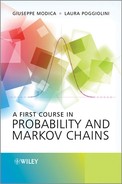
Let us prove the opposite inequality. For ![]() > 0, let
> 0, let ![]() be such that F (yi + δi) ≤ F(yi) +
be such that F (yi + δi) ≤ F(yi) + ![]() 2–i. The open intervals ]xi, yi + δi[ form an open covering of [a +
2–i. The open intervals ]xi, yi + δi[ form an open covering of [a + ![]() , b], hence finitely many among them cover again [a +
, b], hence finitely many among them cover again [a + ![]() , b]. Therefore, by the finite subadditivity of ζ,
, b]. Therefore, by the finite subadditivity of ζ,
Letting ![]() go to zero, we conclude
go to zero, we conclude
![]()
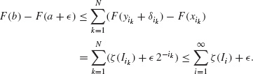
Example B.13 If F is not right-continuous, the set function ζ : ![]() →
→ ![]() , ζ(]a, b]) := F(b) − F (a) is not in general subadditive. For instance, for 0 ≤ a ≤ 1, set
, ζ(]a, b]) := F(b) − F (a) is not in general subadditive. For instance, for 0 ≤ a ≤ 1, set
Let ![]() , clearly
, clearly ![]() , but
, but
![]()
as soon as a < 1.
Theorem B.14 (Lebesgue) The following hold:
(i) Let (![]() (
(![]() ),
), ![]() ) be a finite measure on
) be a finite measure on ![]() . Then the law F (t) :=
. Then the law F (t) := ![]() (] − ∞, t]), t
(] − ∞, t]), t ![]()
![]() , is real valued, monotone nondecreasing and right-continuous.
, is real valued, monotone nondecreasing and right-continuous.
(ii) Let F : ![]() →
→ ![]() be a real valued, monotone nonderecreasing and right-continuous function. Then there exists a unique measure (
be a real valued, monotone nonderecreasing and right-continuous function. Then there exists a unique measure (![]() (
(![]() ),
), ![]() ) finite on bounded sets of
) finite on bounded sets of ![]() such that
such that
![]()
Proof. (i) F is real valued since (![]() (
(![]() ),
), ![]() ) is finite on bounded Borel sets. Moreover, monotonicity property of measures implies that F is monotone nondecreasing. Let us prove that F is right-continuous. Let t
) is finite on bounded Borel sets. Moreover, monotonicity property of measures implies that F is monotone nondecreasing. Let us prove that F is right-continuous. Let t ![]()
![]() and let
and let ![]() be a monotone decreasing sequence such that tn ↓ t. Since ] − ∞, t] =
be a monotone decreasing sequence such that tn ↓ t. Since ] − ∞, t] = ![]() and
and ![]() is finite, one gets F(tn) =
is finite, one gets F(tn) = ![]() (] − ∞, tn]) →
(] − ∞, tn]) → ![]() (] − ∞, t]) = F(t) by the continuity property of measures.
(] − ∞, t]) = F(t) by the continuity property of measures.
(ii) Assume F (t) is right-continuous and monotone nondecreasing. Let ![]() be the semiring of right-closed intervals. The set function
be the semiring of right-closed intervals. The set function ![]() , ζ([a, b]) := F (b) − F (a) is σ-additive, see Proposition B.12. Therefore Theorem B.6 and B.10 apply and ζ extends in a unique way to a measure on the σ-algebra generated by
, ζ([a, b]) := F (b) − F (a) is σ-additive, see Proposition B.12. Therefore Theorem B.6 and B.10 apply and ζ extends in a unique way to a measure on the σ-algebra generated by ![]() , i.e. on
, i.e. on ![]() (
(![]() ), that is finite on bounded open sets.
), that is finite on bounded open sets.
The measure (![]() (
(![]() ),
),![]() ) in Theorem B.14 is called the Stieltjes–Lebesgue measure associated with the right-continuous monotone nondecreasing function F.
) in Theorem B.14 is called the Stieltjes–Lebesgue measure associated with the right-continuous monotone nondecreasing function F.
B.1.2.5 Approximation of Borel sets
Borel sets are quite complicated if compared with open sets that are simply denumerable unions of closed cubes with disjoint interiors. However, the following holds.
Theorem B.15 Let ![]() be a measure on
be a measure on ![]() that is finite on bounded open sets. Then for any
that is finite on bounded open sets. Then for any ![]()
In particular, if ![]() has finite measure,
has finite measure, ![]() (E) < +∞, then for every
(E) < +∞, then for every ![]() > 0 there exists an open set Ω and a compact set K such that K ⊂ E ⊂ Ω and
> 0 there exists an open set Ω and a compact set K such that K ⊂ E ⊂ Ω and ![]() (Ω K) <
(Ω K) < ![]() .
.
Although the result can be derived from (iii) of Theorem B.10, it is actually independent of it. We give here a proof that does not use Theorem B.10.
Proof. Step 1. Let us prove the claim assuming ![]() is finite. Consider the family
is finite. Consider the family
![]()
Of course, ![]() contains the family of open sets. We prove that
contains the family of open sets. We prove that ![]() is closed under denumerable unions and intersections. Let
is closed under denumerable unions and intersections. Let ![]() and, for
and, for ![]() > 0 and j = 1, 2, . . ., let Aj be open sets with Aj ⊃ Ej and
> 0 and j = 1, 2, . . ., let Aj be open sets with Aj ⊃ Ej and ![]() (Aj) ≤
(Aj) ≤ ![]() (Ej) +
(Ej) + ![]() 2–j, that we rewrite as
2–j, that we rewrite as ![]() (Aj Ej) <
(Aj Ej) < ![]() 2–j since Ej and Aj are measurable with finite measure. Since
2–j since Ej and Aj are measurable with finite measure. Since
![]()
we infer
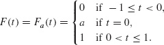
where A := ∪j Aj and B := ∩j Aj. Since A is open and A ⊃ ∪j Ej, the first inequality of (B.10) yields ∪j Ej ![]()
![]() . On the other hand,
. On the other hand, ![]() is open, contains ∩j Ej and, by the second inequality of (B.10),
is open, contains ∩j Ej and, by the second inequality of (B.10), ![]() for sufficiently large N. Therefore ∩j Ej
for sufficiently large N. Therefore ∩j Ej ![]()
![]() .
.
Moreover, since every closed set is the intersection of a denumerable family of open sets, ![]() also contains all closed sets. In particular, the family
also contains all closed sets. In particular, the family
![]()
is a σ-algebra that contains the family of open sets. Consequently, ![]()
![]() and (B.8) holds for all Borel sets of Ω.
and (B.8) holds for all Borel sets of Ω.
Since (B.9) for E is (B.8) for Ec, we have also proved (B.9).
Step 2. Let us prove (B.8) and (B.9) for measures that are finite on bounded open sets. Let us introduce the following notation: given a Borel set ![]() , define the restriction of
, define the restriction of ![]() to A as the set function
to A as the set function
It is easily seen that ![]() is a measure on
is a measure on ![]() that is finite if
that is finite if ![]() (A) < ∞.
(A) < ∞.
Let us prove (B.8). We may assume ![]() (E) < +∞ since otherwise (B.8) is trivial. Let Vj := B(0, j) be the open ball centred at 0 or radius j. The measures
(E) < +∞ since otherwise (B.8) is trivial. Let Vj := B(0, j) be the open ball centred at 0 or radius j. The measures ![]() are Borel and
are Borel and ![]() . Step 1 then yields that for any
. Step 1 then yields that for any ![]() > 0 there are open sets Aj with Aj ⊃ E and
> 0 there are open sets Aj with Aj ⊃ E and ![]() . The set A := ∪j(Aj ∩ Vj) is open, A ⊃ E and, by the subadditivity of
. The set A := ∪j(Aj ∩ Vj) is open, A ⊃ E and, by the subadditivity of ![]()
Let us prove (B.9). The claim easily follows applying Step 1 to the measure ![]() If
If ![]() (E) < +∞. IF
(E) < +∞. IF ![]() (E) = +∞, then E = ∪j Ej with Ej measurable
(E) = +∞, then E = ∪j Ej with Ej measurable ![]() (Ej) < +∞, then for every
(Ej) < +∞, then for every ![]() > 0 and every j there exists a closed set Fj with Fj ⊂ Ej and
> 0 and every j there exists a closed set Fj with Fj ⊂ Ej and ![]() . The set F := ∪j Fj is contained in E and
. The set F := ∪j Fj is contained in E and
![]()
hence, for sufficiently large N, ![]() is closed and
is closed and ![]() .
.
Step 3. By assumption, ![]() and
and ![]() (E) < + ∞. By Step 2 for each
(E) < + ∞. By Step 2 for each ![]() > 0 there exists an open set Ω and a closed set F such that F ⊂ E ⊂ Ω and
> 0 there exists an open set Ω and a closed set F such that F ⊂ E ⊂ Ω and
![]() , so that
, so that ![]() . Setting K :=
. Setting K := ![]() with large enough n, we still get
with large enough n, we still get
![]()
thus concluding that A ⊃ E ⊃ K and ![]() (A K) < 3
(A K) < 3 ![]() .
.
B.1.3 Exercises
Exercise B.16 Show that ![]() (
(![]() ) is the smallest σ-algebra generated by one of the following families of sets:
) is the smallest σ-algebra generated by one of the following families of sets:
- the closed sets;
- the open intervals;
- the closed intervals;
- the intervals ]a, b], a, b
 , a < b;
 - the intervals [a, b[, a, b , a < b;
- the closed half-lines ] − ∞, t], t .
Solution. [Hint. Show that any open set can be written as the union of an at most denumerable family of intervals.]
Exercise B.17 The law of a finite measure ![]() on
on ![]() is defined by
is defined by
![]()
Show that two finite measures ![]() and
and ![]() on
on ![]() coincide if and only if the corresponding laws agree.
coincide if and only if the corresponding laws agree.
B.2 Measurable functions and integration
Characterizing the class of Riemann integrable functions and understanding the range of applicability of the fundamental theorem of calculus were the problems that led to measures and to a more general notion of integral due to Henri Lebesgue (1875–1941). The approach we follow here, which is very well adapted to calculus of probability, is to start with a measure and define the associated notion of integral.
The basic idea is the following. Suppose one wants to compute the area of the subgraph of a non-negative function f : ![]() →
→ ![]() . One can do it by approximating the subgraph in two different ways, see Figure B.1. One can take partitions of the x axis, and approximate the integral by the area of a piecewise constant function as we do when defining the Riemann integral, or one can take a partition of the y axis, and approximate the area of the subgraph by the areas of the strips. The latter defines the area of the subgraph as
. One can do it by approximating the subgraph in two different ways, see Figure B.1. One can take partitions of the x axis, and approximate the integral by the area of a piecewise constant function as we do when defining the Riemann integral, or one can take a partition of the y axis, and approximate the area of the subgraph by the areas of the strips. The latter defines the area of the subgraph as
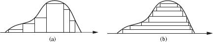
Figure B.1 The computation of an integral according to (a) Riemann and (b) Lebesgue.
where
![]()
is the t upper level of f and |Ef,t| denotes its ‘measure’. Since t → |Ef,t| is monotone nonincreasing, hence Riemann integrable, (B.12) suggests defining the integral by means of the Cavalieri formula
From this point of view, it is clear that the notion of integral makes essential use of a measure on the domain, that must be able to measure even irregular sets, since the upper levels can be very irregular, for instance if the function is oscillating.
In the following, instead of defining the integral by means of (B.13), we adopt a slightly more direct approach to the integral and then prove (B.13).
B.2.1 Measurable functions
Definition B.18 Let ![]() be a σ-algebra of subsets of a set Ω. We say that
be a σ-algebra of subsets of a set Ω. We say that ![]() is
is ![]() -measurable if for any t
-measurable if for any t ![]()
![]() we have
we have
![]()
There are several equivalent ways to say that a function is ![]() -measurable. Taking advantage of the fact that
-measurable. Taking advantage of the fact that ![]() is a σ-algebra, one proves that the following are equivalent:
is a σ-algebra, one proves that the following are equivalent:
(i) {x ![]() Ω | f (x) > t}
Ω | f (x) > t} ![]()
![]() for any t.
for any t.
(ii) {x ![]() Ω | f (x) ≥ t}
Ω | f (x) ≥ t} ![]()
![]() for any t.
for any t.
(iii) {x ![]() Ω | f (x) ≤ t}
Ω | f (x) ≤ t} ![]()
![]() for any t.
for any t.
(iv) {x ![]() Ω | f (x) < t}
Ω | f (x) < t} ![]()
![]() for any t.
for any t.
Moreover, in the previous statements one can substitute ‘for any t’ with ‘for any t in a dense subset of ![]() ’, in particular, with ‘for any t
’, in particular, with ‘for any t ![]()
![]() ’.
’.
Since any open set of ![]() is an at most denumerable union of intervals, the following are also equivalent:
is an at most denumerable union of intervals, the following are also equivalent:
(i) {x ![]() Ω | f (x) > t}
Ω | f (x) > t} ![]()
![]() for any t.
for any t.
(ii) For any open set A ⊂ ![]() we have f−1 (A)
we have f−1 (A) ![]()
![]() .
.
(iii) For any closed F ⊂ ![]() we have f−1 (F)
we have f−1 (F) ![]()
![]() .
.
(iv) For any Borel set B ⊂ ![]() we have f−1(B)
we have f−1(B) ![]()
![]() .
.
The three last statements are independent of the ordering relation of ![]() . They suggest the following extension.
. They suggest the following extension.
Definition B.19 Let ![]() be a σ-algebra of subsets of a set Ω. A vector valued function
be a σ-algebra of subsets of a set Ω. A vector valued function ![]() , N ≥ 1, is
, N ≥ 1, is ![]() -measurable if one of the following holds:
-measurable if one of the following holds:
(i) For any open set A ⊂ ![]() we have f−1(A)
we have f−1(A) ![]()
![]() .
.
(ii) For any closed set F ⊂ ![]() we have f−1(F)
we have f−1(F) ![]()
![]() .
.
(iii) For any Borel set B ⊂ ![]() we have f−1(B)
we have f−1(B) ![]()
![]() .
.
In general, not every function is ![]() -measurable. However, since
-measurable. However, since ![]() is a σ-algebra, one can prove that the algebraic manipulations as well as the pointwise limits of
is a σ-algebra, one can prove that the algebraic manipulations as well as the pointwise limits of ![]() -measurable functions always result in
-measurable functions always result in ![]() -measurable functions. For instance, if f and g are
-measurable functions. For instance, if f and g are ![]() -measurable and α
-measurable and α ![]()
![]() , then the functions
, then the functions
![]()
are ![]() -measurable. Moreover, let
-measurable. Moreover, let ![]() be a sequence of
be a sequence of ![]() -measurable functions. Then:
-measurable functions. Then:
- The functions

are
-measurable. - Let ⊂ Ω be the set
and let f (x) := limn→∞ fn(x), x
E. Then E and for any t we have {x E | f (x) > t} .
Recalling that a function ![]() : X → Y between metric spaces is continuous if and only if for any open set A ⊂ Y the set
: X → Y between metric spaces is continuous if and only if for any open set A ⊂ Y the set ![]() −1 (A) ⊂ X is open, we get immediately the following:
−1 (A) ⊂ X is open, we get immediately the following:
- Continuous functions g : N → m are
 -measurable,
 - Let
 be -measurable and let
  be - measurable, then
  ○ f is -measurable.
In particular, (ii) implies that |f|p, log |f |, . . . are ![]() -measurable functions if f is
-measurable functions if f is ![]() -measurable and that
-measurable and that ![]() , f = (f1, . . ., fN) is
, f = (f1, . . ., fN) is ![]() -measurable if and only if its components f1, . . ., fN are
-measurable if and only if its components f1, . . ., fN are ![]() -measurable.
-measurable.
Let (![]() ,
, ![]() ) be a measure on Ω. A simple function φ : Ω →
) be a measure on Ω. A simple function φ : Ω → ![]() is a function with a finite range and
is a function with a finite range and ![]() -measurable level sets, that is,
-measurable level sets, that is,

The class of simple functions will be denoted by ![]() . Simple functions being linear combinations of
. Simple functions being linear combinations of ![]() -measurable functions are
-measurable functions are ![]() -measurable.
-measurable.
Proposition B.20 (Sampling) Let ![]() be a σ-algebra of subsets of a set Ω. A non-negative function
be a σ-algebra of subsets of a set Ω. A non-negative function ![]() is
is ![]() -measurable if and only if there exists a nondecreasing sequence
-measurable if and only if there exists a nondecreasing sequence ![]() of non-negative simple functions such that φk(x) ↑ f(x) ∀x
of non-negative simple functions such that φk(x) ↑ f(x) ∀x ![]() Ω.
Ω.
Proof. Let f be the pointwise limit of a sequence ![]() of simple functions. Since every φk is
of simple functions. Since every φk is ![]() -measurable, then f is
-measurable, then f is ![]() -measurable.
-measurable.
Conversely, let f : Ω → ![]() be a function. By sampling f, we then construct a sequence
be a function. By sampling f, we then construct a sequence ![]() of functions with finite range approaching f, see Figure B.1. More precisely, let
of functions with finite range approaching f, see Figure B.1. More precisely, let ![]() and for h = 0, 1,, . . . 4k − 1, let
and for h = 0, 1,, . . . 4k − 1, let
![]()
Define φk: Ω → ![]() as
as
By definition, ![]() , moreover,
, moreover, ![]() , since passing from k to k + 1 we half the sampling intervals. Let us prove that
, since passing from k to k + 1 we half the sampling intervals. Let us prove that ![]() . If f (x) = +∞, then φk(x) = 2k ∀k, hence φk(x) → +∞ = f(x). If f(x) < +∞, then for sufficiently large k, f(x) ≤ 2k, hence there exists
. If f (x) = +∞, then φk(x) = 2k ∀k, hence φk(x) → +∞ = f(x). If f(x) < +∞, then for sufficiently large k, f(x) ≤ 2k, hence there exists ![]() such that x
such that x ![]() Ek,h. Therefore,
Ek,h. Therefore,
![]()
Passing to the limit as k → ∞ we get again φk(x) → f(x).
The previous construction applies to any non-negative function ![]() . To conclude, notice that if f is
. To conclude, notice that if f is ![]() -measurable, then the sets Ek and Ek,h are
-measurable, then the sets Ek and Ek,h are ![]() -measurable for every k, h. Since
-measurable for every k, h. Since

φk is a simple function.
B.2.2 The integral
Let (![]() ,
, ![]() ) be a measure on Ω. For any simple function φ : Ω →
) be a measure on Ω. For any simple function φ : Ω → ![]() , one defines the integral of φ with respect to the measure (
, one defines the integral of φ with respect to the measure (![]() ,
, ![]() ) as
) as

as intuition suggests. Since a priori ![]() (φ = aj) may be infinite, we adopt the convention that aj
(φ = aj) may be infinite, we adopt the convention that aj![]() (φ = aj) := 0 if aj = 0. Notice that the integral may be infinite.
(φ = aj) := 0 if aj = 0. Notice that the integral may be infinite.
We then define the integral of a non-negative ![]() -measurable function with respect to (
-measurable function with respect to (![]() ,
, ![]() ) as
) as
For a generic ![]() -measurable function
-measurable function ![]() , decompose f as f(x) = f+(x) − f−(x) where
, decompose f as f(x) = f+(x) − f−(x) where
f+(x) := max(f (x), 0), f−(x) := max(−f(x), 0),
and define
provided that at least one of the integrals on the right-hand side of (B.17) is finite. In this case one says that f is integrable with respect to (![]() ,
, ![]() ). If both the integrals on the right-hand side of (B.17) are finite, then one says that f is summable. Notice that for functions that do not change sign, integrability is equivalent to measurability.
). If both the integrals on the right-hand side of (B.17) are finite, then one says that f is summable. Notice that for functions that do not change sign, integrability is equivalent to measurability.
Since |f(x)| = f+(x) + f−(x) and f+(x), f−(x) ≤ |f(x)|, it is easy to check that if f is ![]() -measurable then so is |f|, and f is summable if and only if f is
-measurable then so is |f|, and f is summable if and only if f is ![]() -measurable and
-measurable and ![]() . Moreover,
. Moreover,
![]()
The class of summable functions will be denoted by ![]() or simply by
or simply by ![]() when the measure is understood.
when the measure is understood.
When ![]() , one refers to the integral with respect to the Lebesgue measure
, one refers to the integral with respect to the Lebesgue measure ![]() in (B.17) as the Lebesgue integral.
in (B.17) as the Lebesgue integral.
Finally, let f : Ω → ![]() be a function and let E
be a function and let E ![]()
![]() . One says that f is measurable on E, integrable on E, and summable on E if f(x)χE(x) is
. One says that f is measurable on E, integrable on E, and summable on E if f(x)χE(x) is ![]() -measurable, integrable, and summable, respectively. If f is integrable on E, one sets
-measurable, integrable, and summable, respectively. If f is integrable on E, one sets
In particular,
![]()
B.2.3 Properties of the integral
From the definition of integral with respect to the measure (![]() ,
, ![]() ) and taking also advantage of the σ-additivity of the measure one gets the following.
) and taking also advantage of the σ-additivity of the measure one gets the following.
Theorem B.21 Let (![]() ,
, ![]() ) be a measure on Ω.
) be a measure on Ω.
(i) For any c ![]()
![]() and f integrable on E, we have
and f integrable on E, we have ![]()
![]() .
.
(ii) (Monotonicity) Let f, g be two integrable functions such that f(x) ≤ g(x) ∀ x ![]() Ω. Then
Ω. Then
![]()
(iii) (Continuity, the Beppo Levi theorem) Let ![]() be a nondecreasing sequence of non-negative
be a nondecreasing sequence of non-negative ![]() -measurable functions
-measurable functions ![]() and let f(x) := limk→∞ fk(x) be the pointwise limit of the fk’s. Then f is integrable and
and let f(x) := limk→∞ fk(x) be the pointwise limit of the fk’s. Then f is integrable and
(iv) (Linearity) ![]() is a vector space and the integral is a linear operator on it: for f,
is a vector space and the integral is a linear operator on it: for f, ![]() and α, β
and α, β ![]()
![]() we have
we have
![]()
A few comments on the Beppo Levi theorem are appropriate. Notice that the measurability assumption is on the sequence ![]() . The measurability of the limit f is for free, thanks to the fact that
. The measurability of the limit f is for free, thanks to the fact that ![]() is a σ-algebra. Moreover, the integrals in (B.19) may be infinite, and the equality is in both directions: we can compute one side of the equality in (B.19) and conclude that the other side has the same value. The Beppo Levi theorem is of course strictly related to the continuity property of measures, and at the end, to the σ-additivity of measures.
is a σ-algebra. Moreover, the integrals in (B.19) may be infinite, and the equality is in both directions: we can compute one side of the equality in (B.19) and conclude that the other side has the same value. The Beppo Levi theorem is of course strictly related to the continuity property of measures, and at the end, to the σ-additivity of measures.
Proof of theorem B.21. (i) and (ii) are trivial.
(iii) Let us prove the Beppo Levi theorem. Since f is the pointwise limit of ![]() -measurable functions, f is
-measurable functions, f is ![]() -measurable. Moreover, since fk(x) ≤ f(x) for any x
-measurable. Moreover, since fk(x) ≤ f(x) for any x ![]() Ω and every k, from (i) we infer
Ω and every k, from (i) we infer ![]() . We now prove the opposite inequality
. We now prove the opposite inequality
![]()
Assume without loss of generality that α < +∞. Let ![]() be a simple function,
be a simple function, ![]() , such that
, such that ![]() ≤ f and let β be a real number, 0 < β < 1. For k = 1, 2, ... set
≤ f and let β be a real number, 0 < β < 1. For k = 1, 2, ... set
![]()
![]() is a nondecreasing sequence of measurable sets such that ∪k Ak = Ω. Hence, from (B.15) and the continuity property of measures
is a nondecreasing sequence of measurable sets such that ∪k Ak = Ω. Hence, from (B.15) and the continuity property of measures
as k → ∞. On the other hand, for any k we have

Therefore, passing to the limit first as k → ∞ in (B.20) and then letting β → 1− we get
![]()
Since the previous inequality holds for any simple function ![]() below f, the definition of integral yields
below f, the definition of integral yields ![]() , as required.
, as required.
(iv) We have already proved the linearity of the integral on the class of simple functions, see Proposition 2.28. To prove (iv), it suffices to approximate f and g by simple functions, see Proposition B.20, and then pass to the limit using (iii).
We conclude with a few simple consequences.
Proposition B.22 Let (![]() ,
, ![]() ) be a measure on Ω.
) be a measure on Ω.
(i) Let E ![]()
![]() have finite measure and let f :
have finite measure and let f : ![]() →
→ ![]() be an integrable function on E
be an integrable function on E ![]()
![]() such that |f(x)| ≤ M for any x
such that |f(x)| ≤ M for any x ![]() E. Then f is summable on E and
E. Then f is summable on E and ![]() .
.
(ii) Let E, F ![]()
![]() and let f : E ∪ F →
and let f : E ∪ F → ![]() be an integrable function on E ∪ F. Then f is integrable both on E and F and
be an integrable function on E ∪ F. Then f is integrable both on E and F and

B.2.4 Cavalieri formula
Theorem B.23 (Cavalieri formula) Let (![]() ,
, ![]() ) be a measure on Ω. For any non-negative
) be a measure on Ω. For any non-negative ![]() -measurable function
-measurable function ![]() we have
we have
As usual, we shorten the notation ![]() ({x
({x ![]() Ω | f(x) > t}) to
Ω | f(x) > t}) to ![]() (f > t).
(f > t).
Proof. Let us prove the claim for non-negative simple functions. Assume ![]() , where the sets
, where the sets ![]() are measurable and pairwise disjoint. For i = 1, . . ., N let
are measurable and pairwise disjoint. For i = 1, . . ., N let ![]() . For the piecewise (hence simple) function
. For the piecewise (hence simple) function ![]() we have
we have
![]()
hence, integrating with respect to t
Assume now f : Ω → ![]() is non-negative and
is non-negative and ![]() -measurable. Proposition B.20 yields a nondecreasing sequence
-measurable. Proposition B.20 yields a nondecreasing sequence ![]() of non-negative simple functions such that φk(x) ↑ f(x) pointwisely. As shown before, for each k = 1, 2, . . .
of non-negative simple functions such that φk(x) ↑ f(x) pointwisely. As shown before, for each k = 1, 2, . . .
![]()
Since φk ↑ f(x) and ![]() (φk > t) ↑
(φk > t) ↑ ![]() (f > t) as k goes to ∞, we can pass to the limit in the previous equality using the Beppo Levi theorem to get
(f > t) as k goes to ∞, we can pass to the limit in the previous equality using the Beppo Levi theorem to get
![]()
The claim then follows, t → ![]() (f > t), being nondecreasing, is Riemann integrable and Riemann and Lebesgue integrals of Riemann integrable functions coincide.
(f > t), being nondecreasing, is Riemann integrable and Riemann and Lebesgue integrals of Riemann integrable functions coincide.
Corollary B.24 Let f : Ω → ![]() be integrable and for any t
be integrable and for any t ![]()
![]() , let F (t) :=
, let F (t) := ![]() (f ≤ t). Then
(f ≤ t). Then
![]()
Proof. Apply (B.22) to the positive and negative parts of f and sum the resulting equalities.
B.2.5 Markov inequality
Let (![]() ,
, ![]() ) be a measure on Ω. From the monotonicity of the integral one deduces that for any non-negative measurable function f : Ω →
) be a measure on Ω. From the monotonicity of the integral one deduces that for any non-negative measurable function f : Ω → ![]() we have the inequality
we have the inequality
![]()
i.e.
This last inequality has different names: Markov inequality, weak estimate or Chebyshev inequality.
B.2.6 Null sets and the integral
Let (![]() ,
, ![]() ) be a measure on Ω.
) be a measure on Ω.
Definition B.25 We say that a set N ⊂ Ω is a null set if there exists F ![]()
![]() such that N ⊂ F and
such that N ⊂ F and ![]() (F) = 0. We say that a predicate p(x), x
(F) = 0. We say that a predicate p(x), x ![]() Ω, is true for
Ω, is true for ![]() -almost every x or
-almost every x or ![]() -a.e., and we write ‘p(x) is true a.e.’ if the set
-a.e., and we write ‘p(x) is true a.e.’ if the set
![]()
is a null set.
In particular, given an ![]() -measurable function f : Ω →
-measurable function f : Ω → ![]() , we say that ‘f = 0
, we say that ‘f = 0 ![]() -a.e.’ or that ‘f(x) = 0 for
-a.e.’ or that ‘f(x) = 0 for ![]() -almost every x
-almost every x ![]() Ω’ if the set {x
Ω’ if the set {x ![]() Ω | f(x) ≠ 0} has zero measure,
Ω | f(x) ≠ 0} has zero measure,
![]()
Similarly, one says that ‘|f| ≤ M ![]() -a.e.’ or that ‘|f(x)| ≤ M for
-a.e.’ or that ‘|f(x)| ≤ M for ![]() -almost every x’, if
-almost every x’, if ![]() ({x
({x ![]() Ω || f(x)| > M}) = 0. From the σ-additivity of the measure, we immediately get the following.
Ω || f(x)| > M}) = 0. From the σ-additivity of the measure, we immediately get the following.
Proposition B.26 Let (![]() ,
, ![]() ) be a measure on Ω and let f : Ω →
) be a measure on Ω and let f : Ω → ![]() be a
be a ![]() -measurable function.
-measurable function.
(i) If ![]() , then |f(x)| < +∞
, then |f(x)| < +∞ ![]() -a.e.
-a.e.
(ii) ![]() if and only if f(x) = 0 for
if and only if f(x) = 0 for ![]() -almost every x
-almost every x ![]() Ω.
Ω.
Proof. (i) Let ![]() . Markov inequality yields for any positive integer k
. Markov inequality yields for any positive integer k
![]()
Hence, passing to the limit as k → ∞ we infer that ![]() ({x
({x ![]() Ω | f(x) = +∞}) = 0.
Ω | f(x) = +∞}) = 0.
(ii) If f(x) = 0 for almost every x ![]() Ω, then every simple function φ such that φ ≤ |f|, is nonzero on at most a null set. Thus
Ω, then every simple function φ such that φ ≤ |f|, is nonzero on at most a null set. Thus ![]() and, by the definition of the integral of |f|,
and, by the definition of the integral of |f|, ![]() .
.
Conversely, from the Markov inequality we get for any positive integer k
![]()
so that ![]() ({x
({x ![]() Ω ||f(x)| > 1/k}) = 0. Since
Ω ||f(x)| > 1/k}) = 0. Since
![]()
passing to the limit as k → ∞ thanks to the continuity property of the measure, we conclude that ![]() ({x
({x ![]() Ω ||f(x)| > 0}) = 0, i.e. |f(x)| = 0
Ω ||f(x)| > 0}) = 0, i.e. |f(x)| = 0 ![]() -a.e.
-a.e.
B.2.7 Push forward of a measure
Let (![]() ,
, ![]() ) be a measure on Ω and let
) be a measure on Ω and let ![]() be an
be an ![]() -measurable function. Since inverse images of Borel sets are
-measurable function. Since inverse images of Borel sets are ![]() -measurable, we define a set function
-measurable, we define a set function ![]() on
on ![]() , also denoted by f#
, also denoted by f#![]() , by
, by
called the pushforward or image of the measure ![]() . It is easy to check the following.
. It is easy to check the following.
Proposition B.27 ![]() is a measure on
is a measure on ![]() and for every non-negative Borel function φ on
and for every non-negative Borel function φ on ![]() we have
we have
Proof. We essentially repeat the proof of Theorem 3.9. For the reader’s convenience, we outline it again.
The σ-additivity of f#![]() follows from the σ-additivity of
follows from the σ-additivity of ![]() using the De Morgan formulas and the relations
using the De Morgan formulas and the relations
![]()
which are true for any family of subsets ![]() of
of ![]() .
.
In order to prove (B.25), we first consider the case in which φ is a simple function, ![]() where c1, ..., cn are distinct constants and the level sets
where c1, ..., cn are distinct constants and the level sets ![]() , i = 1, ..., n, are measurable. then
, i = 1, ..., n, are measurable. then
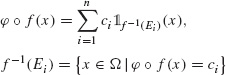
so that
i.e. (B.25) holds when φ is simple.
Let now φ be a non-negative measurable function. Proposition B.20 yields an increasing sequence ![]() of simple functions pointwisely converging to φ. Since for every k we have already proved that
of simple functions pointwisely converging to φ. Since for every k we have already proved that
![]()
we can pass to the limit as k → ∞ and take advantage of the Beppo Levi theorem to get (B.25).
Pushforward of measures can be composed. Let (![]() ,
, ![]() ) be a measure on Ω, let
) be a measure on Ω, let ![]() be
be ![]() -measurable and let
-measurable and let ![]() be
be ![]() (
(![]() N)-measurable. Then from (B.24) we infer
N)-measurable. Then from (B.24) we infer
From (B.25) we infer the following relations for the associated integrals
for every non-negative, ![]() -measurable function
-measurable function ![]() , see Theorem 4.6.
, see Theorem 4.6.
B.2.8 Exercises
Exercise B.28 Let ![]() be a σ-algebra of subsets of a set Ω and let f, g : Ω →
be a σ-algebra of subsets of a set Ω and let f, g : Ω → ![]() be
be ![]() -measurable. Then {x ∈ Ω | f (x) > g(x)}
-measurable. Then {x ∈ Ω | f (x) > g(x)} ![]()
![]() .
.
Solution. For any rational number r ![]()
![]() , the set Ar := {x
, the set Ar := {x ![]() Ω | f (x) > r, g(x) < r} belongs to
Ω | f (x) > r, g(x) < r} belongs to ![]() . Moreover,
. Moreover,
![]()
Thus {x ![]()
![]() | f (x) > g(x)} is a denumerable union of sets in
| f (x) > g(x)} is a denumerable union of sets in ![]() .
.
Exercise B.29 Let ![]() be a σ-algebra of subsets of a set Ω, let E
be a σ-algebra of subsets of a set Ω, let E ![]()
![]() and let f, g : Ω →
and let f, g : Ω → ![]() be two
be two ![]() -measurable functions. Then the function
-measurable functions. Then the function
![]()
is ![]() -measurable.
-measurable.
Exercise B.30 Let ![]() be a σ-algebra of subsets of a set Ω, let f : Ω →
be a σ-algebra of subsets of a set Ω, let f : Ω → ![]() be
be ![]() -measurable and let E
-measurable and let E ![]()
![]() be such that
be such that ![]() (E) < ∞. Then
(E) < ∞. Then ![]() for at most a denumerable set of t’s.
for at most a denumerable set of t’s.
Exercise B.31 Show that if φ is a simple function, then ![]() .
.
Exercise B.32 (Discrete value functions) Let (![]() ,
, ![]() ) be a measure on a set Ω. Let X : Ω →
) be a measure on a set Ω. Let X : Ω → ![]() be an
be an ![]() -measurable non-negative function with discrete values, i.e. X(Ω) is a countable set
-measurable non-negative function with discrete values, i.e. X(Ω) is a countable set ![]() . Give an explicit formula for
. Give an explicit formula for ![]() .
.
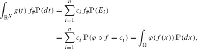
Solution. Let ![]() . Then
. Then
![]()
Given x, the series has only one addendum since only one set Ej contains x.
If X has a finite range, then X is a simple function so that by definition
If X(Ω) is denumerable, then for any non-negative integer k we have

Since X is non-negative, we can apply the Beppo Levi theorem and, as k → ∞, we get
Formula (B.29) can also be written as
since ![]() (X = t) = 0 if
(X = t) = 0 if ![]() .
.
Exercise B.33 Let (![]() ,
, ![]() ) be a measure on a set Ω and let X : Ω →
) be a measure on a set Ω and let X : Ω → ![]() be an
be an ![]() -measurable non-negative function with discrete values and such that +∞
-measurable non-negative function with discrete values and such that +∞ ![]() X(Ω). Give an explicit formula for
X(Ω). Give an explicit formula for ![]() .
.
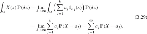
Solution. Let ![]() ∪ {+∞} be the range of X. For k ≥ 1, let Ek := {x | X(x) = ak}, so that
∪ {+∞} be the range of X. For k ≥ 1, let Ek := {x | X(x) = ak}, so that
![]()
and ![]() . From Exercise B.32,
. From Exercise B.32,
![]()
Moreover,
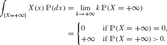
Thus
![]()
Exercise B.34 (Integral on countable sets) Let (![]() ,
, ![]() ) be a measure on a finite or denumerable set Ω. Denote by p : Ω →
) be a measure on a finite or denumerable set Ω. Denote by p : Ω → ![]() , p(x) :=
, p(x) := ![]() ({x}), its mass density. Let X : Ω →
({x}), its mass density. Let X : Ω → ![]() be a non-negative function. Give an explicit formula for
be a non-negative function. Give an explicit formula for ![]() .
.
Solution. Let ![]() be the range of X. By (B.29)
be the range of X. By (B.29)

Exercise B.35 (Dirac delta) Let Ω be a set and let x0 ![]() Ω. The set function
Ω. The set function ![]() such that
such that
![]()
is called the Dirac delta [named after Paul Dirac (1902–1984)] at x0, and is a probability measure on Ω. Prove that for any X : Ω → ![]() ,
,
Exercise B.36 (Sum of measures) Let (![]() , α) and (
, α) and (![]() , β) be two measures on Ω and let λ,
, β) be two measures on Ω and let λ, ![]() .
.
(i) Show that λα + μβ : ![]() →
→ ![]() defined by (λα + μβ)(E) := λα(E) + μβ(E) ∀E
defined by (λα + μβ)(E) := λα(E) + μβ(E) ∀E ![]()
![]() is such that (
is such that (![]() , λα + μβ) is a measure on Ω.
, λα + μβ) is a measure on Ω.
(ii) Show that for amy ![]() -measurable non-negative function
-measurable non-negative function ![]()
Solution. We first consider the case when f is a non-negative simple function: ![]() where
where ![]() , ci ≥ 0. Thus
, ci ≥ 0. Thus

When f is an ![]() -measurable non-negative function, we approximate it from below with an increasing sequence
-measurable non-negative function, we approximate it from below with an increasing sequence ![]() of simple functions that pointwise converges to f(x). Since any φk is simple, we have
of simple functions that pointwise converges to f(x). Since any φk is simple, we have
![]()
Letting k → +∞ and taking advantage of the Beppo Levi theorem we get (B.32).
Example B.37 (Counting measure) Let Ω be a set. Given a subset A ⊂ Ω let ![]() 0(A) := |A| be the cardinality of A. It is easy to see that (
0(A) := |A| be the cardinality of A. It is easy to see that (![]() (Ω),
(Ω), ![]() 0) is a measure on Ω, called counting measure. Clearly,
0) is a measure on Ω, called counting measure. Clearly,
![]()
where the sum on the right-hand side is +∞ if A has infinite many points. The corresponding integral is
![]()
The formula above is obvious if f is nonzero on a finite set only and can be proven by passing to the limit and taking advantage of the Beppo Levi theorem in the general case.
Exercise B.38 (Absolutely continuous measures) Let ![]() (
(![]() ,
, ![]() ) be an absolutely continuous measure with respect to the Lebesgue measure, i.e. assume there exists a summable function
) be an absolutely continuous measure with respect to the Lebesgue measure, i.e. assume there exists a summable function ![]() such that
such that
![]()
Show that, for any non-negative ![]() (
(![]() )-measurable function f,
)-measurable function f,
Solution. Assume f is simple, i.e. ![]()
![]() . Then
. Then

The general case can be proven by an approximation argument, using Proposition B.20 and the Beppo Levi theorem.
B.3 Product measures and iterated integrals
B.3.1 Product measures
Let (![]() ,
, ![]() ) and (
) and (![]() ,
, ![]() ) be measures on two sets X and Y, respectively. Denote by
) be measures on two sets X and Y, respectively. Denote by ![]() the family of all ‘rectangles’ in the Cartesian product X × Y
the family of all ‘rectangles’ in the Cartesian product X × Y
![]()
and let ![]() be the set function that maps any rectangle A × B
be the set function that maps any rectangle A × B ![]()
![]() into ζ(A × B) :=
into ζ(A × B) := ![]() (A)
(A)![]() (B). The following can be easily shown.
(B). The following can be easily shown.
Proposition B.39 ![]() is a semiring and ζ :
is a semiring and ζ : ![]() →
→ ![]() is a σ-additive set function.
is a σ-additive set function.
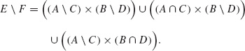
Proof. It is quite trivial to show that ![]() is a semiring. In fact, if E := A × B and F := C × D
is a semiring. In fact, if E := A × B and F := C × D ![]()
![]() , then E ∩ F = (A ∩ C) × (B ∩ D) and
, then E ∩ F = (A ∩ C) × (B ∩ D) and
Let us prove that ζ is σ-additive. Let ![]() × F = ∪k(Ek × Fk), E, Ek
× F = ∪k(Ek × Fk), E, Ek ![]()
![]() , F, Fk
, F, Fk ![]()
![]() be such that the sets
be such that the sets ![]() are pairwise disjoint so that
are pairwise disjoint so that
![]()
Integrating with respect to ![]() on Y and applying the Beppo Levi theorem, we obtain
on Y and applying the Beppo Levi theorem, we obtain
![]()
Moreover, integrating with respect to ![]() on X and again by the Beppo Levi theorem we get
on X and again by the Beppo Levi theorem we get
![]()
Thus, see Theorem B.10, ζ extends to a measure denoted (![]() ,
, ![]() ×
× ![]() ) on the smallest σ-algebra
) on the smallest σ-algebra ![]() containing
containing ![]() . This measure is called the product measure of (
. This measure is called the product measure of (![]() ,
, ![]() ) and (
) and (![]() ,
, ![]() ). Moreover, such an extension is unique, provided ζ :
). Moreover, such an extension is unique, provided ζ : ![]() →
→ ![]() + is σ-finite, see Theorem B.6. This happens in particular, if both (
+ is σ-finite, see Theorem B.6. This happens in particular, if both (![]() ,
, ![]() ) and (
) and (![]() ,
, ![]() ) are σ-finite.
) are σ-finite.
Of course one can consider the product of finitely many measures. Taking for instance the product of n Bernoulli trials, one obtains the Bernoulli distribution on {0, 1}n
![]()
B.3.1.1 Infinite Bernoulli process
Let (Ω, ![]() ,
, ![]() ) be a probability measure on Ω. Consider the set
) be a probability measure on Ω. Consider the set ![]() of Ω-valued sequences, and consider the family
of Ω-valued sequences, and consider the family ![]() ⊂
⊂ ![]() (Ω∞) of sets E ⊂ Ω∞ of the form
(Ω∞) of sets E ⊂ Ω∞ of the form
![]()
where Ei ![]()
![]() ∀i and Ei = Ω except for a finite number of indexes, i.e. the family of ‘cylinders’ with the terminology of Section 2.2.7. Define also α :
∀i and Ei = Ω except for a finite number of indexes, i.e. the family of ‘cylinders’ with the terminology of Section 2.2.7. Define also α : ![]() → [0, 1] by setting for
→ [0, 1] by setting for ![]() ,
,
![]()
Notice that the product is actually a finite product, since ![]() (Ei) = 1 except for a finite number of indexes.
(Ei) = 1 except for a finite number of indexes.
The following theorem holds. The interested reader may find a proof in, e.g. [7].
Theorem B.40 (Kolmogorov) ![]() is a semiring and α is σ-additive on
is a semiring and α is σ-additive on ![]() .
.
Therefore, Theorem B.6 and B.10 apply so that there exists a unique probability measure (![]() ,
, ![]() ∞) on Ω∞ that extends α to the σ-algebra generated by
∞) on Ω∞ that extends α to the σ-algebra generated by ![]() .
.
The existence and uniqueness of the Bernoulli distribution of parameter p introduced in Section 2.2.7 is a particular case of the previous statement. One obtains it by choosing the Bernoulli trial distribution B(1, p) on {0, 1} as starting probability space (Ω, ![]() ,
, ![]() ).
).
B.3.2 Reduction formulas
Let A ⊂ X × Y. For any point x ![]() A let Ax be the subset of Y defined as
A let Ax be the subset of Y defined as
![]()
Ax is called the section of A at x.
Theorem B.41 (Fubini) Let X, Y be two sets and let (![]() ,
, ![]() ×
× ![]() ) be the product measure on X × Y of the two σ-finite measures (
) be the product measure on X × Y of the two σ-finite measures (![]() ,
, ![]() ) and (
) and (![]() ,
, ![]() ) on X and Y, respectively. Then, for any A
) on X and Y, respectively. Then, for any A ![]()
![]() the following hold:
the following hold:
(i) Ax ![]()
![]()
![]() -a.e. x
-a.e. x ![]() X.
X.
(ii) x ![]()
![]() (Ax) is an
(Ax) is an ![]() -measurable function.
-measurable function.
(iii) ![]() .
.
Changing the roles of the two variables, one also has:
(iv) Ay ![]()
![]()
![]() -a.e. y
-a.e. y ![]() Y.
Y.
(v) y ![]()
![]() (Ay) is an
(Ay) is an ![]() -measurable function.
-measurable function.
(vi) ![]() .
.
From the Fubini theorem, Theorem B.41, one obtains the following reduction formulas.
Theorem B.42 (Fubini–Tonelli) Let (![]() ,
, ![]() ) and (
) and (![]() ,
, ![]() ) be two σ-finite measures on the sets X and Y, respectively, and let (
) be two σ-finite measures on the sets X and Y, respectively, and let (![]() ,
, ![]() ×
× ![]() ) be the product measure on X × Y. Let f : X × Y →
) be the product measure on X × Y. Let f : X × Y → ![]() be
be ![]() -measurable and non-negative (respectively,
-measurable and non-negative (respectively, ![]() ×
× ![]() summable). Then the following hold:
summable). Then the following hold:
(i) y ![]() f (x, y) is
f (x, y) is ![]() -measurable (respectively,
-measurable (respectively, ![]() -summable)
-summable) ![]() -a.e. x
-a.e. x ![]() X.
X.
(ii) ![]() is
is ![]() -measurable (respectively,
-measurable (respectively, ![]() -summable).
-summable).
![]()
Of course, the two variables can be interchanged, so under the same assumption of Theorem B.42 we also have:
(i) x ![]() f(x, y) is
f(x, y) is ![]() -measurable (respectively,
-measurable (respectively, ![]() -summable)
-summable) ![]() -a.e. y
-a.e. y ![]() Y.
Y.
(ii) ![]() is
is ![]() -measurable (respectively,
-measurable (respectively, ![]() -summable).
-summable).
(iii) We have
![]()
Proof. The proof is done in three steps.
(i) If f is the characteristic function of a ![]() ×
× ![]() measurable set, then we apply the Fubini theorem, Theorem B.41. Because of additivity, the result still holds true for any
measurable set, then we apply the Fubini theorem, Theorem B.41. Because of additivity, the result still holds true for any ![]() -measurable simple function f.
-measurable simple function f.
(ii) If f is non-negative, then f can be approximated from below by an increasing sequence of simple functions. Applying the Beppo Levi theorem and the continuity of measures, the result holds true for f.
(iii) If f is ![]() ×
× ![]() summable, then one applies the result of Step (ii) to the positive and negative parts f+ and f− of f.
summable, then one applies the result of Step (ii) to the positive and negative parts f+ and f− of f.
Notice that the finiteness assumption on the two measures (![]() ,
, ![]() ) and (
) and (![]() ,
, ![]() ) in Theorems B.41 and B.42 cannot be dropped as the following example shows.
) in Theorems B.41 and B.42 cannot be dropped as the following example shows.
Example B.43 Let X = Y = ![]() ,
, ![]() , and let
, and let ![]() be the measure that counts the points:
be the measure that counts the points: ![]() (A) = |A|. Let S := {(x, x) | x
(A) = |A|. Let S := {(x, x) | x ![]() [0, 1]} and let f(x, y) = χS(x, y) be its characteristic function. S is closed, hence S belongs to the smallest σ-algebra generated by ‘intervals’, i.e.
[0, 1]} and let f(x, y) = χS(x, y) be its characteristic function. S is closed, hence S belongs to the smallest σ-algebra generated by ‘intervals’, i.e. ![]() (
(![]() 2). Clearly (
2). Clearly (![]() ×
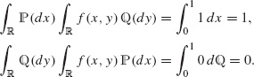
× ![]() )(S) = ∞, but
)(S) = ∞, but
B.3.3 Exercises
Exercise B.44 Show that ![]() on the Borel sets of
on the Borel sets of ![]() .
.
Exercise B.45 Let (![]() ,
, ![]() ) be a measure on Ω and let
) be a measure on Ω and let ![]() be a
be a ![]() -measurable function. Show that the subgraph of f
-measurable function. Show that the subgraph of f
![]()
is ![]() ×
× ![]() -measurable and
-measurable and
![]()
[Hint. Prove the claim for simple functions and use an approximation argument for the general case.]
B.4 Convergence theorems
B.4.1 Almost everywhere convergence
Definition B.46 Let (![]() ,
, ![]() ) be a measure on Ω and let
) be a measure on Ω and let ![]() and X be
and X be ![]() -measurable functions.
-measurable functions.
(i) We say that ![]() converges in measure to X, if for any δ > 0
converges in measure to X, if for any δ > 0
![]()
(ii) We say that ![]() converges to X almost everywhere, and we write Xn → X
converges to X almost everywhere, and we write Xn → X ![]() -a.e., if the measure of the set
-a.e., if the measure of the set
is null, ![]() (E) = 0.
(E) = 0.
The difference between the above defined convergences becomes clear if one first considers the following sets, which can be constructed starting from a given sequence of sets ![]() ; namely, the sets
; namely, the sets
![]()
In the following proposition we collect the elementary properties of such sets.
Proposition B.47 We have the following:
(i) x ![]() lim infn An if and only if there exists
lim infn An if and only if there exists ![]() such that x
such that x ![]() An ∀n ≥
An ∀n ≥ ![]() .
.
(ii) x ![]() lim supn An if and only if there exists infinite values of n such that x
lim supn An if and only if there exists infinite values of n such that x ![]() An.
An.
(iii) x ![]() (Ωlim supn An)c if and only if
(Ωlim supn An)c if and only if ![]() is finite.
is finite.
(iv) ![]() .
.
(v) Let ![]() be a σ-algebra of subsets of Ω. If
be a σ-algebra of subsets of Ω. If ![]() ⊂
⊂ ![]() , then both lim infn An and lim supn An are
, then both lim infn An and lim supn An are ![]() -measurable. Moreover,
-measurable. Moreover,
![]()
Proof. (i) and (ii) agree with the definitions of lim infn An and lim supn An, respectively. (iii) is a rewrite of (ii) and (iv) is a consequence of De Moivre formulas. To prove (v) it suffices to observe that the ![]() -measurability of lim infn An and lim supn An comes from the properties of σ-algebras and that the inequality in (v) is a consequence of the continuity of measures.
-measurability of lim infn An and lim supn An comes from the properties of σ-algebras and that the inequality in (v) is a consequence of the continuity of measures.
Let (![]() ,
, ![]() ) be a measure on Ω and let
) be a measure on Ω and let ![]() and X be
and X be ![]() -measurable functions. Given any δ ≥ 0, define
-measurable functions. Given any δ ≥ 0, define

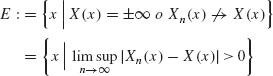
Since x ![]() Eδ if and only if there exists a sequence
Eδ if and only if there exists a sequence ![]() such that |Xkn(x) − X(x)| > δ, then
such that |Xkn(x) − X(x)| > δ, then
Proposition B.48 Let (![]() ,
, ![]() ) be a measure on Ω and let
) be a measure on Ω and let ![]() and X be
and X be ![]() -measurable functions. With the notation above,
-measurable functions. With the notation above, ![]() converges to X in measure if and only if
converges to X in measure if and only if ![]() (An,δ) → 0 as n → ∞ for any positive δ. Moreover, the following are equivalent:
(An,δ) → 0 as n → ∞ for any positive δ. Moreover, the following are equivalent:
(i) Xn → X ![]() -a.e.
-a.e.
(ii) ![]() (lim supn An,0) = 0.
(lim supn An,0) = 0.
(iii) ![]() (lim supn An,δ) = 0 for any δ > 0.
(lim supn An,δ) = 0 for any δ > 0.
Proof. By definition, Xn → X ![]() -a.e. if and only if
-a.e. if and only if ![]() (E0) = 0. For any δ ≥ 0, Eδ ⊂ E0 = ∪δ >0 Eδ, hence
(E0) = 0. For any δ ≥ 0, Eδ ⊂ E0 = ∪δ >0 Eδ, hence ![]() (E0) = 0 if and only if
(E0) = 0 if and only if ![]() (Eδ) = 0 for any δ > 0. The claim follows from (B.34).
(Eδ) = 0 for any δ > 0. The claim follows from (B.34).
Convergence in measure and almost everywhere convergence are not equivalent, see Example 4.76. Nevertheless, the two convergences are related, as the following proposition shows.
Proposition B.49 Let (![]() ,
, ![]() ) be a measure on Ω and let
) be a measure on Ω and let ![]() and X be
and X be ![]() -measurable functions on Ω. Then:
-measurable functions on Ω. Then:
(i) If Xn → X ![]() -a.e., then Xn → X in measure.
-a.e., then Xn → X in measure.
(ii) If Xn → X in measure, then there exists a subsequence ![]() of
of ![]() such that Xkn → X
such that Xkn → X ![]() -a.e.
-a.e.
Proof. (i) Let δ > 0. For any n let ![]() . By Proposition B.48,
. By Proposition B.48, ![]() for any δ > 0. Let m ≥ 1 and define
for any δ > 0. Let m ≥ 1 and define ![]()
![]() . Then An,δ ⊂ Bm ∀n ≥ m hence
. Then An,δ ⊂ Bm ∀n ≥ m hence
![]()
(ii) Let ![]() . We must show that there exists a sequence nj such that
. We must show that there exists a sequence nj such that
![]()
see Definition 4.75 and (B.34). Let ![]() . By assumption
. By assumption ![]() (An,δ) → 0 for any δ > 0. Let n1 be the smallest integer such that
(An,δ) → 0 for any δ > 0. Let n1 be the smallest integer such that ![]() , and for any k ≥ 2, let nk+1 be the smallest integer greater than nk such that
, and for any k ≥ 2, let nk+1 be the smallest integer greater than nk such that ![]() . Let
. Let ![]() . Since Bm ↓ ∩mBm = lim supj(Anj,1/j) we obtain
. Since Bm ↓ ∩mBm = lim supj(Anj,1/j) we obtain
![]()
Since
![]()
the claim follows.
B.4.2 Strong convergence
We see here some different results related to the Beppo Levi theorem and the convergence of integrals.
The first result is about the convergence of integrals of series of non-negative functions.
Proposition B.50 (Series of non-negative functions) Let (![]() ,
, ![]() ) be a measure on Ω. Let
) be a measure on Ω. Let ![]() be a sequence of
be a sequence of ![]() -measurable non-negative functions. Then
-measurable non-negative functions. Then
![]()
Proof. The partial sums ![]() are a nondecreasing sequence of
are a nondecreasing sequence of ![]() -measurable non-negative functions. Applying the Beppo Levi theorem to this sequence yields the result.
-measurable non-negative functions. Applying the Beppo Levi theorem to this sequence yields the result.
B.4.3 Fatou lemma
In the following lemma, the monotonicity assumption in the Beppo Levi theorem is removed.
Lemma B.51 (Fatou) Let (![]() ,
, ![]() ) be a measure on Ω and let
) be a measure on Ω and let ![]() be a sequence of
be a sequence of ![]() -measurable non-negative functions. Then
-measurable non-negative functions. Then
![]()
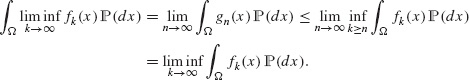
Proof. Let gn(x) := infk≥n fk(x). ![]() is an increasing sequence of
is an increasing sequence of ![]() -measurable non-negative functions. Moreover,
-measurable non-negative functions. Moreover,
![]()
Thus ![]() and, applying the Beppo Levi theorem, we get
and, applying the Beppo Levi theorem, we get
Remark B.52 The Fatou lemma implies the Beppo Levi theorem. In fact, let ![]() be an increasing sequence of functions that converges to f(x). Then f(x) = limk→∞ fk(x) = lim infk→∞ fk(x). Since the sequence
be an increasing sequence of functions that converges to f(x). Then f(x) = limk→∞ fk(x) = lim infk→∞ fk(x). Since the sequence ![]() is monotone, we get
is monotone, we get
![]()
and, by the Fatou lemma, we get the opposite inequality:
![]()
Corollary B.53 (Fatou lemma) Let (![]() ,
, ![]() ) be a measure on Ω. Let
) be a measure on Ω. Let ![]() be a sequence of
be a sequence of ![]() -measurable functions and let
-measurable functions and let ![]() : Ω →
: Ω → ![]() be a
be a ![]() -summable function.
-summable function.
(i) If fk(x) ≥ ![]() (x) ∀k and
(x) ∀k and ![]() -a.e. x
-a.e. x ![]() Ω, then
Ω, then
![]()
(ii) If fk(x) ≤ ![]() (x) ∀k and
(x) ∀k and ![]() -a.e., then
-a.e., then
![]()
Proof. Let ![]() and let E := ∩k Ek. Since
and let E := ∩k Ek. Since ![]() (Ec) = 0, we can assume without loss of generality that fk(x) ≥
(Ec) = 0, we can assume without loss of generality that fk(x) ≥ ![]() (x) ∀k and ∀x
(x) ∀k and ∀x ![]() Ω. To prove (i) it suffices to apply the Fatou lemma, Lemma B.51, to the sequence
Ω. To prove (i) it suffices to apply the Fatou lemma, Lemma B.51, to the sequence ![]() . (ii) is proven similarly.
. (ii) is proven similarly.
B.4.4 Dominated convergence theorem
Theorem B.54 (Lebesgue dominated convergence) Let (![]() ,
, ![]() ) be a measure on Ω and let
) be a measure on Ω and let ![]() be a sequence of
be a sequence of ![]() -measurable functions. Assume:
-measurable functions. Assume:
(i) fk(x) → f(x) ![]() -a.e. x
-a.e. x ![]() Ω.
Ω.
(ii) There exists a ![]() -summable function
-summable function ![]() such that |fk(x)| ≤
such that |fk(x)| ≤ ![]() (x) ∀k and for
(x) ∀k and for ![]() -a.e. x.
-a.e. x.
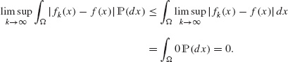
Then
![]()
and, in particular,
![]()
Proof. By assumption |fk(x) − f(x)| ≤ 2![]() (x) for
(x) for ![]() -a.e. x and for any k. Moreover, |fk(x) − f(x)| → 0 ∀k and for
-a.e. x and for any k. Moreover, |fk(x) − f(x)| → 0 ∀k and for ![]() -a.e. x. Thus, by the Fatou lemma, Corollary B.53, we get
-a.e. x. Thus, by the Fatou lemma, Corollary B.53, we get
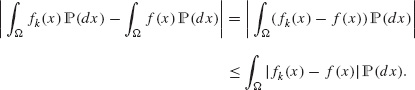
The last claim is proven by the following inequality:
Remark B.55 Notice that in Theorem B.54:
- Assumption (ii) is equivalent to the
 -summability of the envelope (x) := supk |fk(x)| of the functions |fk|.
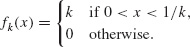
 - Assumption (ii) cannot be dropped as the following sequence
 shows:
Example B.56 The dominated convergence theorem extends to arbitrary measures a classical dominated convergence theorem for series.
Theorem (Dominated convergence for series) Let ![]() be a double sequence such that:
be a double sequence such that:
(i) For any j, aj,n → aj as n → ∞.
(ii) There exists a non-negative sequence ![]() such that |aj,n| ≤ cj for any n and any j and
such that |aj,n| ≤ cj for any n and any j and ![]() .
.
Then the series ![]() is absolutely convergent and
is absolutely convergent and
![]()
Proof. Consider the counting measure ![]() on Ω =
on Ω = ![]() and apply the Lebesgue dominated convergence theorem to the sequence
and apply the Lebesgue dominated convergence theorem to the sequence ![]() defined by fn(j) = aj,n.
defined by fn(j) = aj,n.
For the reader’s convenience, we include a direct proof. Since aj,n → aj and |an,j| ≤ cj ∀n, j, we get |aj| ≤ cj ∀j so that ![]() is absolutely convergent.
is absolutely convergent.
Let ![]() > 0. Choose p = p(
> 0. Choose p = p(![]() ) such that
) such that ![]() . Then
. Then
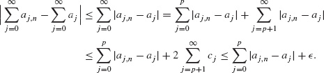
Thus, as n → ∞, we obtain
![]()
Since ![]() is arbitrary, the claim follows.
is arbitrary, the claim follows.
The next theorem is an important consequence on the convergence of integrals of series of functions.
Theorem B.57 (Lebesgue) Let (![]() ,
, ![]() ) be a measure on Ω and let
) be a measure on Ω and let ![]() be a sequence of
be a sequence of ![]() -measurable functions such that
-measurable functions such that
![]()
Then for ![]() -a.e. x the series
-a.e. x the series ![]() is absolutely convergent to a
is absolutely convergent to a ![]() -summable function f(x). Moreover,
-summable function f(x). Moreover,
and
![]()
Notice that the assumptions are on the integrals only, while the claim is about the ![]() -a.e. convergence of the series
-a.e. convergence of the series ![]() .
.
Proof. For any x ![]() Ω let
Ω let ![]() be the sum of the non-negative addenda series
be the sum of the non-negative addenda series ![]() . Applying the Beppo Levi theorem, the assumption gives
. Applying the Beppo Levi theorem, the assumption gives
![]()
i.e. g is ![]() -summable. Thus, by Proposition B.26, g(x) < +∞ for
-summable. Thus, by Proposition B.26, g(x) < +∞ for ![]() -a.e. x, i.e. the series
-a.e. x, i.e. the series ![]() absolutely converges to
absolutely converges to ![]() and, for any integer p ≥ 1 we have
and, for any integer p ≥ 1 we have
In particular,
![]()
so that f is summable. Integrating (B.36) we get
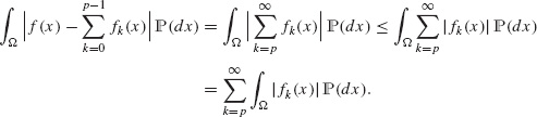
As p → ∞ we get the first part of the claim. The second part of the claim easily follows since

B.4.5 Absolute continuity of integrals
Theorem B.58 (Absolute continuity of integrals) Let (![]() ,
, ![]() ) be a measure on Ω and let f be a
) be a measure on Ω and let f be a ![]() -summable function. For any
-summable function. For any ![]() > 0 there exists δ > 0 such that
> 0 there exists δ > 0 such that ![]() for any E
for any E ![]()
![]() such that
such that ![]() (E) < δ. Equivalently,
(E) < δ. Equivalently,
![]()
Proof. Let

Then |fk(x) − f(x)| → 0 for ![]() -a.e. x and |fk(x) − f(x)| ≤ 2|f(x)|, Since |f| is
-a.e. x and |fk(x) − f(x)| ≤ 2|f(x)|, Since |f| is ![]() -summable, the dominated convergence theorem, Theorem B.54, applies for any
-summable, the dominated convergence theorem, Theorem B.54, applies for any ![]() > 0 there exists
> 0 there exists ![]() such that
such that
![]()
Let δ := ![]() /(2N). Then for any E
/(2N). Then for any E ![]()
![]() such that
such that ![]() (E) ≤ δ we get
(E) ≤ δ we get
![]()
so that
![]()
B.4.6 Differentiation of the integral
Let ![]() be Lebesgue-summable non-negative functions. Clearly,
be Lebesgue-summable non-negative functions. Clearly, ![]() if and only if f(x) = g(x) almost everywhere. Thus one would like to characterize f(x) in terms of its integral, i.e. of the map
if and only if f(x) = g(x) almost everywhere. Thus one would like to characterize f(x) in terms of its integral, i.e. of the map ![]() . Differentiation theory provides such a characterization. Obviously, if f is continuous, then the mean value theorem gives
. Differentiation theory provides such a characterization. Obviously, if f is continuous, then the mean value theorem gives
![]()
More generally, the following theorem holds.
Theorem B.59 (Lebesgue) Let E ⊂ ![]() be a
be a ![]() -measurable set and let f : E →
-measurable set and let f : E → ![]() be
be ![]() -measurable such that
-measurable such that ![]() for some 1 ≤ p < +∞. Then for almost every x
for some 1 ≤ p < +∞. Then for almost every x ![]() E,
E,
![]()
In particular, for almost every x ![]() E, the limit
E, the limit
![]()
exists, is finite and equal to f(x).
Example B.60 Let f be ![]() -summable on ] − 1, 1[. Show that
-summable on ] − 1, 1[. Show that
![]()
Definition B.61 Let ![]() be
be ![]() -summable on E. The points of the set
-summable on E. The points of the set
![]()
are called Lebesgue points of f. For any ![]() the limit
the limit
![]()
exists and is finite thus it defines a function ![]() called the Lebesgue representative of f.
called the Lebesgue representative of f.
From the Lebesgue differentiation theorem, Theorem B.59, we get
Theorem B.62 Let f be a ![]() -summable function on
-summable function on ![]() . Then
. Then ![]() and f = λf
and f = λf ![]() -a.e.
-a.e.
The differentiation theorem can be extended to more general sets than balls centred at x. One may use cubes centred at x, cubes containing x or even different objects. For example, let A be a bounded Borel set such that ![]() (A) > 0. Assume, e.g.
(A) > 0. Assume, e.g.
![]()
For any x ![]()
![]() and any r > 0, let Ax,r := x + r A. Obviously, Ax,r ⊂ B(x, 100 r) and |Ax,r| = rn |A| = crn |B1| = c |B(x, r)|. Theorem B.59 implies the following.
and any r > 0, let Ax,r := x + r A. Obviously, Ax,r ⊂ B(x, 100 r) and |Ax,r| = rn |A| = crn |B1| = c |B(x, r)|. Theorem B.59 implies the following.
Theorem B.63 Let E ⊂ ![]() be a Borel-measurable set and let f : E →
be a Borel-measurable set and let f : E → ![]() be
be ![]() -measurable with
-measurable with ![]() for some 1 ≤ p < ∞. Then for
for some 1 ≤ p < ∞. Then for ![]() -a.e. x
-a.e. x ![]() E
E
![]()
We now collect some results due to Giuseppe Vitali (1875–1932) on the differentiation of integrals and of monotone functions.
Theorem B.64 (Vitali) Let h : ![]() →
→ ![]() be monotone nondecreasing. Then h is differentiable at
be monotone nondecreasing. Then h is differentiable at ![]() -a.e. x
-a.e. x ![]()
![]() and the derivative h′(x) is non-negative at
and the derivative h′(x) is non-negative at ![]() -a.e. x
-a.e. x ![]()
![]() . Moreover, h′ is
. Moreover, h′ is ![]() -summable on any bounded interval ]a, b[
-summable on any bounded interval ]a, b[![]()
![]() and
and
Remark B.65 Equality may not hold in (B.37). Take, e.g. h(x) := sgn(x) so that h′(x) = 0 ∀x ≠ 0, and, of course, ![]() . Although surprising, one may construct examples of continuous and strictly increasing functions whose derivative is zero almost everywhere: one somewhat simpler example of a continuous, nonconstant and nondecreasing function with zero derivative almost everywhere is the famous Cantor–Vitali function. Obviously, for such functions the inequality in (B.37) may be strict.
. Although surprising, one may construct examples of continuous and strictly increasing functions whose derivative is zero almost everywhere: one somewhat simpler example of a continuous, nonconstant and nondecreasing function with zero derivative almost everywhere is the famous Cantor–Vitali function. Obviously, for such functions the inequality in (B.37) may be strict.
Definition B.66 A function f : ![]() →
→ ![]() is said to be absolutely continuous if for any
is said to be absolutely continuous if for any ![]() > 0 there exists δ > 0 such that for any pair of sequences
> 0 there exists δ > 0 such that for any pair of sequences ![]() ,
, ![]() such that
such that ![]() we have
we have ![]() .
.
Let f ![]() L1([a, b]), Theorem B.58 implies that the integral function
L1([a, b]), Theorem B.58 implies that the integral function
![]()
is absolutely continuous. The next theorem shows that integral functions are the only absolutely continuous functions.
Theorem B.67 (Vitali) A function h : [a, b] → ![]() is absolutely continuous if and only if there exists a
is absolutely continuous if and only if there exists a ![]() -summable function f on [a, b] such that
-summable function f on [a, b] such that
![]()
Moreover, h is differentiable at almost every x ![]() [a, b] and h′(x) = f(x) for a.e. x
[a, b] and h′(x) = f(x) for a.e. x ![]() [a, b].
[a, b].
Lipschitz continuous functions f : ![]() →
→ ![]() are absolutely continuous; thus by Theorem B.67 they are differentiable
are absolutely continuous; thus by Theorem B.67 they are differentiable ![]() -a.e., the derivative f′(x) is
-a.e., the derivative f′(x) is ![]() -summable and
-summable and
![]()
Moreover, the following holds in ![]() .
.
Theorem B.68 (Rademacher) Let f : ![]() →
→ ![]() be Lipschitz continuous. Then f is differentiable at
be Lipschitz continuous. Then f is differentiable at ![]() -almost every x
-almost every x ![]()
![]() , the map x → D f(x) is
, the map x → D f(x) is ![]() -measurable and |D f(x)| ≤ Lip(f)
-measurable and |D f(x)| ≤ Lip(f) ![]() -a.e. x
-a.e. x ![]()
![]() .
.
B.4.7 Weak convergence of measures
In this section we consider Borel measures on ![]() , that is measures (
, that is measures (![]() (
(![]() ), μ) on
), μ) on ![]() . Since the σ algebra is understood, we simply write μ to denote the measure (
. Since the σ algebra is understood, we simply write μ to denote the measure (![]() (
(![]() ), μ).
), μ).
Recall that the law of a finite Borel measure μ on ![]() is the function F :
is the function F : ![]() →
→ ![]() , F(t) := μ(] − ∞, t]). We recall that F is monotone nondecreasing, in particular, is right-continuous on
, F(t) := μ(] − ∞, t]). We recall that F is monotone nondecreasing, in particular, is right-continuous on ![]() and the set of its discontinuity points is at most denumerable. Moreover, F(t) → F(−∞) as t → −∞ and F(t) → F(+∞) as t → +∞ and the measure μ is completely determined by F.
and the set of its discontinuity points is at most denumerable. Moreover, F(t) → F(−∞) as t → −∞ and F(t) → F(+∞) as t → +∞ and the measure μ is completely determined by F.
Definition B.69 Let ![]() , μ be finite Borel measures on
, μ be finite Borel measures on ![]() . We say that
. We say that ![]() weakly converges to μ, and we write
weakly converges to μ, and we write ![]() , if for any continuous bounded function φ :
, if for any continuous bounded function φ : ![]() →
→ ![]() one has
one has
![]()
Proposition B.70 If the weak limit of a sequence of measures exists, then it is unique.
Proof. Assume ![]() and
and ![]() , and let
, and let ![]() := μ1 – μ2. Then, for every continuous bounded function φ:
:= μ1 – μ2. Then, for every continuous bounded function φ: ![]() →
→ ![]()
![]()
The characteristic function of ] − ∞, a] can be approximated from below by an increasing sequence of continuous non-negative functions, thus obtaining ![]() ([−∞, a]) = 0 ∀
([−∞, a]) = 0 ∀ ![]()
![]() , hence
, hence ![]() (A) = 0 ∀A
(A) = 0 ∀A ![]()
![]() (
(![]() ).
).
Theorem B.71 Let ![]() , μ be a finite Borel measures on
, μ be a finite Borel measures on ![]() . Assume μn(
. Assume μn(![]() ) = μ(
) = μ(![]() ) ∀n and let Fn and F be their laws, respectively. The following are equivalent:
) ∀n and let Fn and F be their laws, respectively. The following are equivalent:
(i) If F is continous at t, then Fn(t) → F(t).
(ii) μn weakly converges to μ.
Proof. (i) ![]() (ii) Without any loss of generality, we can assume that for any n
(ii) Without any loss of generality, we can assume that for any n ![]()
![]() , Fn(−∞) = F(−∞) = 0 and Fn(+∞) = μn(
, Fn(−∞) = F(−∞) = 0 and Fn(+∞) = μn(![]() ) = μ(
) = μ(![]() ) = F(+∞) = 1. Fix δ > 0 and let a, b
) = F(+∞) = 1. Fix δ > 0 and let a, b ![]()
![]() , a < b, such that F is continuous at a and b, and such that F(a) ≤ δ and 1 − F(b) ≤ δ. Fn(a) and Fn(b) converge to F(a) and F(b), respectively, hence for large enough n’s, Fn(a) ≤ 2δ, 1 − Fn(b) ≤ 2δ.
, a < b, such that F is continuous at a and b, and such that F(a) ≤ δ and 1 − F(b) ≤ δ. Fn(a) and Fn(b) converge to F(a) and F(b), respectively, hence for large enough n’s, Fn(a) ≤ 2δ, 1 − Fn(b) ≤ 2δ.
Let φ : ![]() →
→ ![]() be a bounded continuous function, |φ| ≤ M. Since φ is uniformly continuous in [a, b], there exists N = Nδ and intervals Ij = [aj, aj+1], j = 1, . . ., Nδ where a = a1 < a2 < · · · < aN+1 = b such that the oscillation of φ on every Ij is less than δ, maxIj φ − minIj φ ≤ δ∀j. Morever, perturbating the extrema aj if necessary, we can assume that all the points aj are continuity points for F. Let
be a bounded continuous function, |φ| ≤ M. Since φ is uniformly continuous in [a, b], there exists N = Nδ and intervals Ij = [aj, aj+1], j = 1, . . ., Nδ where a = a1 < a2 < · · · < aN+1 = b such that the oscillation of φ on every Ij is less than δ, maxIj φ − minIj φ ≤ δ∀j. Morever, perturbating the extrema aj if necessary, we can assume that all the points aj are continuity points for F. Let ![]() . h is a simple function h|Ij = φ(aj) and h = 0 in
. h is a simple function h|Ij = φ(aj) and h = 0 in ![]() [a, b]. Moreover, |φ(x) − h(x)| ≤ δ on ]a, b]. Since φ is bounded and μn(
[a, b]. Moreover, |φ(x) − h(x)| ≤ δ on ]a, b]. Since φ is bounded and μn(![]() ) = 1,
) = 1,
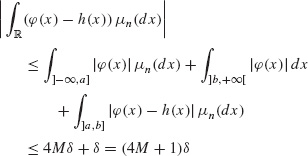
and, similarly,
![]()
hence
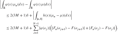
Since Fn(aj) → F(aj) for any j = 1, . . ., N, we get as n → ∞
![]()
Since δ > 0 is arbitrary, the claim is proven.
(ii) ![]() (i) Let a
(i) Let a ![]()
![]() . It suffices to show that
. It suffices to show that
In fact, from (B.38) one gets
![]()
i.e. F(a) = limn→∞ Fn(a) if F is continuous at a.
For any δ > 0, let φ(t) be the piecewise linear function that is null for any t ≥ a and is identically 1 for t ≤ a − δ. Then

As δ → 0+, F(a − δ) → F(a−), so the first inequality in (B.38) is proven. Similarly, let φ(t) be the piecewise linear function that is null for t ≥ a + δ and is identically 1 for t ≤ a. Then
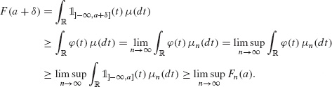
As δ → 0+, F(a + δ) → F(a) so that the second inequality in (B.38) holds. The proof of (B.38) is then complete.
Let (![]() ,
, ![]() ) be a probability measure on a set Ω. We recall that the law FX associated with an
) be a probability measure on a set Ω. We recall that the law FX associated with an ![]() -measurable function X : Ω →
-measurable function X : Ω → ![]() is the law of the image measure of
is the law of the image measure of ![]() through X, i.e.
through X, i.e.
![]()
Definition B.72 Let (![]() ,
, ![]() ) be a finite measure on a set Ω and let
) be a finite measure on a set Ω and let ![]() , X be
, X be ![]() -measurable functions. We say that
-measurable functions. We say that ![]() converges in law to X if FXn (t) converges to FX(t) pointwisely in all points of continuity of FX.
converges in law to X if FXn (t) converges to FX(t) pointwisely in all points of continuity of FX.
Proposition B.73 Let (![]() ,
, ![]() ) be a finite measure on a set Ω and let
) be a finite measure on a set Ω and let ![]() , X be
, X be ![]() -measurable functions. If Xn → X in measure then Xn converges in law to X.
-measurable functions. If Xn → X in measure then Xn converges in law to X.
Proof. If suffices to prove that
In fact, from (B.39) one gets
![]()
hence FX(a) = limn→∞ FXn(a) if FX is continuous at a.
Let us prove (B.39). Let δ > 0. Since
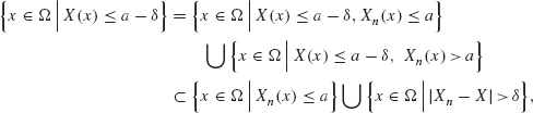
we have
![]()
Thus, passing to the limit with respect to n, we obtain
![]()
If we now let δ → 0+, we get the first inequality (B.39). Similarly,

so that
![]()
As n → ∞ we get
![]()
so that, by letting δ → 0+ we obtain the second inequality of (B.39).
B.4.8 Exercises
Exercise B.74 Let f : ![]() →
→ ![]() be
be ![]() -summable. Prove that the function F :
-summable. Prove that the function F : ![]() × [0, ∞[ →
× [0, ∞[ → ![]() defined by
defined by
![]()
is continuous.
Exercise B.75 Let f ![]() L1(
L1(![]() ). Prove that the following equalities hold for a.e. x
). Prove that the following equalities hold for a.e. x ![]()
![]() :
:
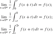
Exercise B.76 Let φ : [a, b] → [c, d] be continuous and piecewise differentiable. Let h : [c, d] → ![]() be absolutely continuous. Prove that f ○ φ : [a, b] →
be absolutely continuous. Prove that f ○ φ : [a, b] → ![]() is absolutely continuous.
is absolutely continuous.
Exercise B.77 Let φ : [a, b] → [c, d] be continuous. Then φ is absolutely continuous if and only if the graph of φ has finite length.
Exercise B.78 Let (![]() ,
, ![]() ) be a measure on a set Ω. Let
) be a measure on a set Ω. Let ![]() , X be
, X be ![]() -measurable functions and let p
-measurable functions and let p ![]() [1, ∞[. Assume that:
[1, ∞[. Assume that:
(i) Xn → X ![]() -a.e. x
-a.e. x ![]() Ω.
Ω.
(ii) ![]() .
.
Prove that ![]() .
.
Solution. For any positive n the function Yn := 2p−1(|X|p + |Xn|p) − |Xn − X|p is non-negative. Moreover, as n → ∞, Yn converges to 2p|X|p ![]() -a.e. Thus, by the Fatou lemma
-a.e. Thus, by the Fatou lemma
