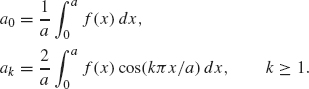
1
FOURIER SERIES
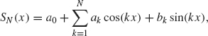
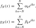
In this chapter, we examine the trigonometric expansion of a function f(x) defined on an interval such as –π ≤ x ≤ π. A trigonometric expansion is a sum of the form
where the sum could be finite or infinite. Why should we care about expressing a function in such a way? As the following sections show, the answer varies depending on the application we have in mind.
1.1.1 Historical Perspective
Trigonometric expansions arose in the 1700s, in connection with the study of vibrating strings and other, similar physical phenomena; they became part of a controversy over what constituted a general solution to such problems, but they were not investigated in any systematic way. In 1808, Fourier wrote the first version of his celebrated memoir on the theory of heat, Théorie Analytique de la Chaleur, which was not published until 1822. In it, he made a detailed study of trigonometric series, which he used to solve a variety of heat conduction problems.
Fourier’s work was controversial at the time, partly because he did make unsubstantiated claims and overstated the scope of his results. In addition, his point of view was new and strange to mathematicians of the day. For instance, in the early 1800s a function was considered to be any expression involving known terms, such as powers of x, exponential functions, and trigonometric functions. The more abstract definition of a function (i.e., as a rule that assigns numbers from one set, called the domain, to another set, called the range) did not come until later. Nineteenth-century mathematicians tried to answer the following question: Can a curve in the plane, which has the property that each vertical line intersects the curve at most once, be described as the graph of a function that can be expressed using powers of x, exponentials, and trigonometric functions. In fact, they showed that for “most curves,” only trigonometric sums of the type given in (1.1) are needed (powers of x, exponentials, and other types of mathematical expressions are unnecessary). We shall prove this result in Theorem 1.22.
The Riemann integral and the Lebesgue integral arose in the study of Fourier series. Applications of Fourier series (and the related Fourier transform) include probability and statistics, signal processing, and quantum mechanics. Nearly two centuries after Fourier’s work, the series that bears his name is still important, practically and theoretically, and still a topic of current research. For a fine historical summary and further references, see John J. Benedetto’s book (Benedetto, 1997).
1.1.2 Signal Analysis
There are many practical reasons for expanding a function as a trigonometric sum. If f(t) is a signal, (for example, a time-dependent electrical voltage or the sound coming from a musical instrument), then a decomposition of f into a trigonometric sum gives a description of its component frequencies. Here, we let t be the independent variable (representing time) instead of x. A sine wave, such as sin(kt), has a period of 2π/k and a frequency of k (i.e., vibrates k times in the interval 0 ≤ t ≤ 2π). A signal such as
![]()
contains frequency components that vibrate at 1, 3, and 200 times per 2π interval length. In view of the size of the coefficients, the component vibrating at a frequency of 3 dominates over the other frequency components.
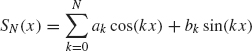
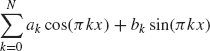
A common task in signal analysis is the elimination of high-frequency noise. One approach is to express f as a trigonometric sum
![]()
and then set the high-frequency coefficients (the ak and bk for large k) equal to zero.
Another common task in signal analysis is data compression. The goal here is to describe a signal in a way that requires minimal data. One approach is to express the signal, f, in terms of a trigonometric expansion, as previously, and then retain only those coefficients, ak and bk, which are larger (in absolute value) than some specified tolerance. The coefficients that are small and do not contribute substantially to f can be thrown away. There is no danger that an infinite number of coefficients stay large, because we will show (see the Riemann-Lebesgue Lemma, Theorem 1.21) that ak and bk converge to zero as k → ∞.
1.1.3 Partial Differential Equations
Trigonometric sums also arise in the study of partial differential equations. Although the subject of partial differential equations is not the main focus of this book, we digress to give a simple yet important example. Consider the heat equation
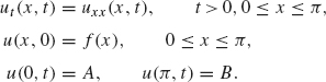
The solution, u(x,t), to this differential equation represents the temperature of a rod of length π at position x and at time t with initial temperature (at t = 0) given by f(x) and where the temperatures at the ends of the rod, x = 0 and x = π, are kept at A and B, respectively. We will compute the solution to this differential equation in the special case where A = 0 and B = 0. The expansion of f into a trigonometric series will play a crucial role in the derivation of the solution.
Separation of Variables. To solve the heat equation, we use the technique of separation of variables which assumes that the solution is of the form
![]()
where T(t) is a function of t ≥ 0 and X(x) is a function of x, 0 ≤ x ≤ π. Inserting this expression for u into the differential equation ut = uxx yields
![]()
or
![]()
The left side depends only on t and the right side depends only on x. The only way these two functions can equal each other for all values of x and t is if both functions are constant (since x and t are independent variables). So, we obtain the following two equations:
![]()
where c is a constant. From the equation T’ = cT, we obtain T(t) = Cect, for some constant C. From physical considerations, the constant c must be negative (otherwise |T(t)| and hence the temperature |u(x, t)| would increase to infinity as t → ∞). So we write c = –λ2 < 0 and we have T(t) = Ce–λ2t. The differential equation for X becomes
![]()
The boundary conditions, X(0) = 0 = X(π) arise because the temperature u(x, t) = X(x)T(t) is assumed to be zero at x = 0, π. The solution to this differential equation is
![]()
The boundary condition X(0) = 0 implies that the constant a must be zero. The boundary condition 0 = X(π) = b sin(λπ) implies that λ must be an integer, which we label k. Note that we do not want to set b equal to zero, because if both a and b were zero, the function X would be zero and hence the temperature u would be zero. This would only make sense if the initial temperature of the rod, f(x), is zero.
To summarize, we have shown that the only allowable value of λ is an integer k with corresponding solutions xk(x) = bk sin(kx) and Tk(t) = e–k2t. Each function
![]()
is a solution to the heat equation and satisfies the boundary condition u(0, t) = u(π, t) = 0. The only missing requirement is the initial condition u(x, 0) = f(x), which we can arrange by considering the sum of the uk:
Setting u(x, t = 0) equal to f(x), we obtain the equation
Equation (1.4) is called a Fourier sine expansion of f. In the coming sections, we describe how to find such expansions (i.e. how to find the bk). Once found, the Fourier coefficients (the bk) can be substituted into Eq. (1.3) to give the final solution to the heat equation.
Thus, the problem of expanding a function in terms of sines and cosines is an important one, not only from a historical perspective, but also for practical problems in signal analysis and partial differential equations.
1.2 COMPUTATION OF FOURIER SERIES
1.2.1 On the Interval –π ≤ x ≤ π
In this section, we will compute the Fourier coefficients, ak and bk, in the Fourier series
![]()
We need the following result on the orthogonality of the trigonometric functions.
Theorem 1.1 The following integral relations hold.
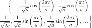
An equivalent way of stating this theorem is that the collection
is an orthonormal set of functions in L2([–π, π]).
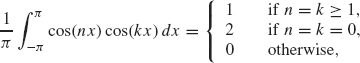
Proof. The derivations of the first two equalities use the following identities:
Adding these two identities and integrating gives
![]()
The right side can be easily integrated, n ≠ k then
![]()
If n = k ≥ 1, then
![]()
If n = k = 0, then Eq. (1.5) reduces to ![]() . This completes the proof of Eq. (1.5).
. This completes the proof of Eq. (1.5).
Equation (1.6) follows by subtracting Eqs. (1.9) and (1.10) and then integrating as before. Equation (1.7) follows from the fact that cos(nx) sin(kx) is odd for k > 0 (see Lemma 1.7).
Now we use the orthogonality relations given in (1.5)–(1.7) to compute the Fourier coefficients. We start with the equation
To find an for n ≥ 1, we multiply both sides by cos nx and integrate:

From Eqs. (1.5)–(1.7), only the cosine terms with n = k contribute to the right side and we obtain
![]()
Similarly, by multiplying Eq. (1.11) by sin nx and integrating, we obtain
![]()
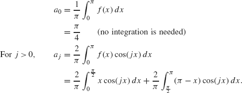
As a special case, we compute a0 by integrating Eq. (1.11) to give
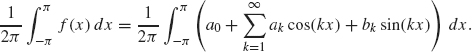
Each sin and cos term integrates to zero and therefore
![]()
We summarize this discussion in the following theorem.
Theorem 1.2 If ![]() , then
, then
The an and bn are called the Fourier coefficients of the function f.
Remark. The crux of the proof of Theorem 1.2 is that the collection in (1.8) is orthonormal. Thus, Theorem 0.21 guarantees that the Fourier coefficients an and bn are obtained by orthogonally projecting f onto the space spanned by cos nx and sin nx, respectively. In fact, note that an and bn are (up to a factor of 1/π) the L2 inner products of f (x) with cos nx and sin nx, respectively, as provided by Theorem 0.21. Thus, the preceding proof is a repeat of the proof of Theorem 0.21 for the special case of the L2-inner product and where the orthonormal collection (the ej) is given in (1.8).
Keep in mind that we have only shown that if f can be expressed as a trigonometric sum, then the coefficients an and bn are given by the preceding formulas. We will show (Theorem 1.22) that most functions can be expressed as trigonometric sums. Note that Theorem 1.2 implies that the Fourier coefficients for a given function are unique.
1.2.2 Other Intervals
Intervals of Length 2π. In Theorem 1.2, the interval of interest is [–π, π]. As we will show in this section, Theorem 1.2 also holds for any interval of length 2π. We will need the following lemma.
Lemma 1.3 Suppose F is any 2π-periodic function and c is any real number, then
Fig. 1.1. Region between –π and –π + c has the same area as between π and π + c.
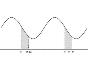
Proof. A simple proof of this lemma is described graphically by Figure 1.1. If F ≥ 0, the left side of Eq. (1.15) represents the area under the graph of F from x = –π + c to x = π + c, whereas the right side of Eq. (1.15) represents the area under the graph of F from x = –π to x = π. Since F is 2π-periodic, the shaded regions in Figure 1.1 are the same. The process of transferring the left shaded region to the right shaded region transforms the integral on the right side of Eq. (1.15) to the left.
An analytical proof of this lemma is outlined in exercise 25.
Using this lemma with F(x) = f(x)cos nx or f(x)sin nx, we see that the integration formulas in Theorem 1.2 hold for any interval of the form [–π + c, + c.
Intervals of General Length. We can also consider intervals of the form –a ≤ x ≤ a, of length 2a. The basic building blocks are cos(nπx/a) and sin(nπx/a), which are 2a/n-periodic. Note that when a = n, these functions reduce to cos nx and sin nx, which form the basis for Fourier series on the interval [–π, π] considered in Theorem 1.2.
The following scaling argument can be used to transform the integral formulas for the Fourier coefficients on the interval [–π, π] to the interval [–a, a]. Suppose F is a function defined on the interval –π ≤ x ≤ π. The substitution x = tπ/a, dx = πdt/a leads to the following change of variables formula:
![]()
By using this change of variables, the following theorem can be derived from Theorem 1.2. (see exercise 15).
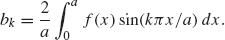
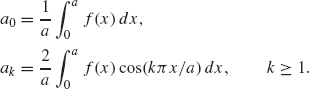
Theorem 1.4 If ![]() on the interval –a ≤ x ≤ a, then
on the interval –a ≤ x ≤ a, then
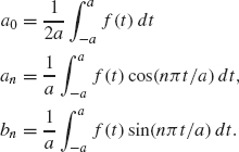
Example 1.5 Let
![]()
We will compute the formal Fourier series for f valid on the interval –2 ≤ x ≤ 2. With a = 2 in Theorem 1.4, the Fourier cosine coefficients are
![]()
and for n ≥ 1
![]()
When n is even, these coefficients are zero. When n = 2k + 1 is odd, then sin(nπ/2) = (–1)k. Therefore
![]()
Similarly,
Thus, the Fourier series for f is
![]()
with an, bn given as above.
In later sections, we take up the question of whether or not the Fourier series F(x) for f equals f(x) itself.
1.2.3 Cosine and Sine Expansions
Even and Odd Functions.
Definition 1.6 Let f : R → R be a function; f is even if f(–x) = f(x); f is odd if f(–x) = –f(x).
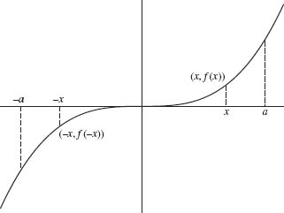
The graph of an even function is symmetric about the y axis as illustrated in Figure 1.2. Examples include f(x) = x2 (or any even power) and f(x) = cos x. The graph of an odd function is symmetric about the origin as illustrated in Figure 1.3. Examples include f (x) = x3 (or any odd power) and f (x) = sin x.
The following properties follow from the definition.
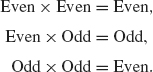
Fig. 1.2. Even function f(–x) = f(x).
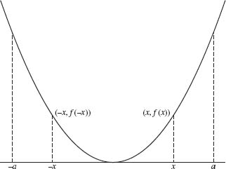
Fig. 1.3. Odd function f(–x) = –f(x).
For example, if f is even and g is odd, then g(–x)f (–x) = –g(x)f(x) and so f g is odd.
Another important property of even and odd functions is given in the next lemma.
Lemma 1.7
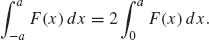
- If F is an even function, then
- If F is an odd function, then
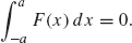
This lemma follows easily from Figures 1.2 and 1.3. If F is even, then the integral over the left half-interval [–a,0] is the same as the integral over the right half interval [0, a]. Thus, the integral over [–a, a] is twice the integral over [0, a]. If F is odd, then the integral over the left half interval [–a, 0] cancels with the integral over the right half-interval [0, a]. In this case, the integral over [–a, a] is zero.
If the Fourier series of a function only involves the cosine terms, then it must be an even function (since cosine is even). Likewise, a Fourier series that only involves sines must be odd. The converse of this is also true, which is the content of the next theorem.
Theorem 1.8
- If f (x) is an even function, then its Fourier series on the [–a, a] will only involve cosines; i.e.,
 , with
- If f(x) is an odd function, then its Fourier series will only involve sines. That is,
 , with
Proof. This theorem follows from Lemma 1.7 and Theorem 1.4. If f is even, then f(x) cos nπx/a is even and so its integral over [–a, a] equals twice the integral over [0, a]. In addition, fsin nπx/a is odd and so its integral over [–a, a] is zero. The second part follows similarly.
Fourier Cosine and Sine Series on a Half Interval. Suppose f is defined on the interval [0, a]. By considering even or odd extensions of f, we can expand f as a cosine or sine series. To express f as a cosine series, we consider the even extension of f:
![]()
The function fe is an even function defined on [–a, a]. Therefore, only cosine terms appear in its Fourier expansion:
where ak is given in Theorem 1.8. Since fe(x) = f(x) for 0 ≤ x ≤ a, the integral formulas in Theorem 1.8 only involve f(x) rather than fe(x) and so Eq. (1.16) becomes
![]()
with
Likewise, if f is odd, then we consider the odd extension of f :
![]()
The odd function, fo, has only sine terms in its Fourier expansion. Since fo(x) = f(x) for 0 ≤ x ≤ a, we obtain the following sine expansion for f
![]()
where bk is given in Theorem 1.8:
![]()
The examples in the next section will clarify these ideas.
1.2.4 Examples
Let f be a function and let F(x) be its Fourier series on [–π, π.
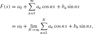
where an and bn are the Fourier coefficients of f. We say that the Fourier series converges if the preceding limit exists (as N → ∞). Theorems 1.2 and 1.4 only compute the Fourier series of a given function. We have not yet shown that a given Fourier series converges (or what it converges to). In Theorems 1.22 and 1.28, we show that under mild hypothesis on the differentiability of f, the following principle holds:
Let f be a 2π-periodic function.
- If f is continuous at a point x, then its Fourier series, F(x), converges and
- If f is not continuous at a point x, then F(x) converges to the average of the left and right limits of f at x, that is,
The second statement includes the first because if f is continuous at x, then the left and right limits of f are both equal to f (x) and so in this case, F(x) = f(x).
Rigorous statements and proofs of Theorems 1.22 and 1.28 are given in the following sections. In this section, we present several examples to gain insight into the computation of Fourier series and the rate at which Fourier series converge.
Example 1.9 Consider the function f(x) = x on –π ≤ x ≤ π. This function is odd and so only the sine coefficients are nonzero. Its Fourier coefficients are
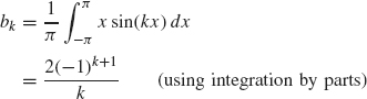
and so its Fourier series for the interval [–≤, ≤] is
![]()
The function f (x) = x is not 2≤-periodic. Its periodic extension, ![]() , is given in Figure 1.4. According to the principle in Eq. (1.17), F(x) converges to
, is given in Figure 1.4. According to the principle in Eq. (1.17), F(x) converges to ![]() (x) at points where
(x) at points where ![]() is continuous. At points of discontinuity (x = … –π, π,… ), F(x) will converge to the average of the left and right limits of
is continuous. At points of discontinuity (x = … –π, π,… ), F(x) will converge to the average of the left and right limits of ![]() (x), see Eq. (1.18). For example, F(π) = 0 (since sin kπ = 0), which is the average of the left and right limit of
(x), see Eq. (1.18). For example, F(π) = 0 (since sin kπ = 0), which is the average of the left and right limit of ![]() at x = π.
at x = π.
To see how fast the partial sums of this Fourier series converges to ![]() (x), we graph the partial sum
(x), we graph the partial sum
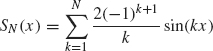
for various values of N. The graph of
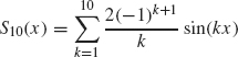
Fig. 1.4. The periodic extension of f (x) = x.
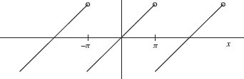
Fig. 1.5. Gibbs phenomenon for S10.
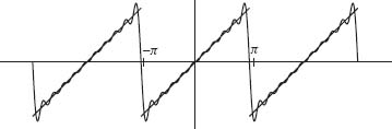
Fig. 1.6. Gibbs phenomenon for S50 in Example 1.9.
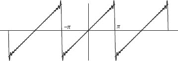
is given in Figure 1.5 together with the graph of ![]() (x) (the squiggly curve is the graph of S10).
(x) (the squiggly curve is the graph of S10).
First, notice that the accuracy of the approximation of ![]() (x) by S10(x) gets worse as x gets closer to a point of discontinuity. For example, near x = π, the graph of S10(x) must travel from about y = π to y = –π in a. very short interval resulting in a slow rate of convergence near x = π.
(x) by S10(x) gets worse as x gets closer to a point of discontinuity. For example, near x = π, the graph of S10(x) must travel from about y = π to y = –π in a. very short interval resulting in a slow rate of convergence near x = π.
Second, notice the blips in the graph of the Fourier series just before and just after the points of discontinuity of f (x) (near x = π for example). This effect is called the Gibbs phenomenon. An interesting fact about the Gibbs phenomenon is that the height of the blip is approximately the same no matter how many terms are considered in the partial sum. However, the width of the blip gets smaller as the number of terms increase. Figure 1.6 illustrates the Gibbs phenomenon for S50 (the first 50 terms of the Fourier expansion) for ![]() . Exercise 32 explains the Gibbs effect in more detail.
. Exercise 32 explains the Gibbs effect in more detail.
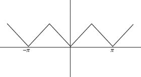
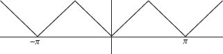
Example 1.10 Consider the sawtooth wave illustrated in Figure 1.7. The formula for f on the interval 0 ≤ x ≤ π is given by
![]()
and extends to the interval –π ≤ x ≤ 0 as an even function (see Figure 1.7).
Fig. 1.7. Sawtooth wave.
Since f is an even function, only the cosine terms are nonzero. Using Theorem 1.8, their coefficients are
After performing the necessary integrals, we have
![]()
Only the a4k+2 are nonzero. These coefficients simplify to
![]()
So the Fourier series for the sawtooth wave is
![]()
The sawtooth wave is already periodic and it is continuous. Thus its Fourier series F(x) equals the sawtooth wave, f (x), for every x by the principle stated at the beginning of this section, see (1.17). In addition, the rate of convergence is much faster than for the Fourier series in Example 1.9. To illustrate the rate of convergence, we plot the sum of the first two terms of its Fourier series
![]()
in Figure 1.8.
The sum of just two terms of this Fourier series gives a more accurate approximation of the sawtooth wave than 10 or 50 or even 1000 terms of the Fourier series in the previous (discontinuous) example. Indeed, the graph of the first 10 terms of this Fourier series (given in Figure 1.9) is almost indistinguishable from the original function.
Example 1.11 Let f(x) = sin(3x) + cos(4x). Since f is already expanded in terms of sines and cosines, no work is needed to compute the Fourier series of f ; that is, the Fourier series of f is just sin(3x) + cos(4x). This example illustrates an important point. The Fourier coefficients are unique (Theorem 1.2 specifies exactly what the ak and bk must be). Thus by inspection, b3 = 1, a4 = 1 and all other ak and bk are zero. By uniqueness, these are the same values as would have been obtained by computing the integrals in Theorem 1.2 for the ak and bk (with much less work).
Fig. 1.8. Sum of first two Terms of the Fourier series of the sawtooth.
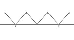
Fig. 1.9. Ten terms of the Fourier series of the sawtooth.
Example 1.12 Let f (x) = sin2(x). In this example, f is not a linear combination of sines and cosines, so there is some work to do. However, instead of computing the integrals in Theorem 1.2 for the ak and bk, we use a trigonometric identity
![]()
The right side is the desired Fourier series for f since it is a linear combination of cos(kx) (here, a0 = 1/2, a2 = –1/2 and all other ak and bkare zero).
Example 1.13 To find the Fourier sine series for the function f(x) = x2 + 1 valid on the interval 0 ≤ x ≤ 1, we first extend f as an odd function:
![]()
Then we use Theorem 1.8 to compute the Fourier coefficients for fo.
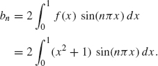
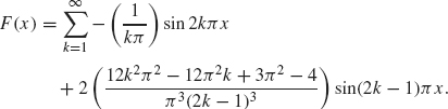
Note that the formula of the odd extension of f to the interval –1 ≤ x ≤ 0 is not needed for the computation of bn. Integration by parts (twice) gives
![]()
When n = 2k is even, this simplifies to
![]()
and when n = 2k – 1 is odd:
![]()
Thus the Fourier sine series for x2 + 1 on the interval [0, 1] is
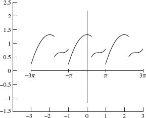
Now fo is defined on the interval [–1, 1]. Its periodic extension, ![]() o is graphed on the interval [–2, 2] in Figure 1.10. Its Fourier series, F(x), will converge to
o is graphed on the interval [–2, 2] in Figure 1.10. Its Fourier series, F(x), will converge to ![]() at each point of continuity of fo. At each integer,
at each point of continuity of fo. At each integer, ![]() is discontinuous. By the principle stated at the beginning of this section [see Eq. (1.18)], F(x) will converge to zero at each integer value (the average of the left and right limits of fo). This agrees with the value of F computed by using Eq. (1.19) (since sin kπx is zero at each integer). A graph of F(x) is given in Figure 1.11. Note that since
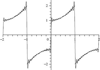
is discontinuous. By the principle stated at the beginning of this section [see Eq. (1.18)], F(x) will converge to zero at each integer value (the average of the left and right limits of fo). This agrees with the value of F computed by using Eq. (1.19) (since sin kπx is zero at each integer). A graph of F(x) is given in Figure 1.11. Note that since ![]() for 0 < x < 1, the Fourier sine series F(x) agrees with f(x) = x2 + 1 on the interval 0 x < 1. A partial sum of the first 30 terms of F(x) is given in Figure 1.12.
for 0 < x < 1, the Fourier sine series F(x) agrees with f(x) = x2 + 1 on the interval 0 x < 1. A partial sum of the first 30 terms of F(x) is given in Figure 1.12.
Fig. 1.10. Periodic odd extension of f(x) = x2 + 1.
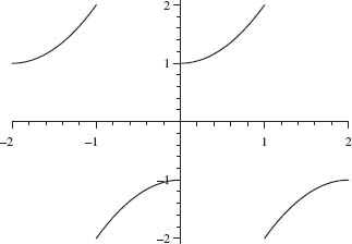
Fig. 1.11. Graph of F, the Fourier sine series of f(x) = x2 + 1.
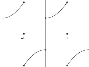
Fig. 1.12. Graph of sum of first 30 terms of F(x).
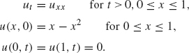
Example 1.14 Solve the heat equation
where f(x) is the sawtooth wave in Example 1.10, that is,
![]()
From the discussion in Section 1.1.3, the solution to this problem is
Setting t = 0 in (1.20) and using u(x, 0) = f(x), we obtain
![]()
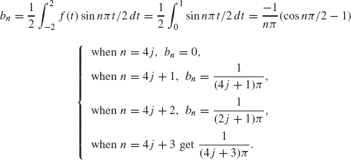
Therefore, the bk must be chosen as the Fourier sine coefficients of f(x), which by Theorem 1.8 are
![]()
Inserting the formula for f and computing the integral, the reader can show bk = 0 when k is even. When k = 2j + 1 is odd, then
![]()
Substituting bk into Eq. (1.20), the final solution is
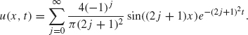
1.2.5 The Complex Form of Fourier Series
Often, it is more convenient to express Fourier series in its complex form using the complex exponentials, einx, n ∈ Z where Z denotes the integers {... –2, –1, 0, 1, 2,...}. The complex exponential has the following definition.
Definition 1.15 For any real number t, the complex exponential is
![]()
where ![]() .
.
This definition is motivated by substituting x = it into the usual Taylor series for ex:
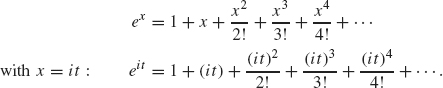
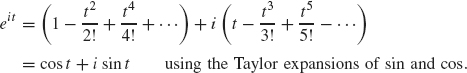
Collecting the real and imaginary parts, we obtain
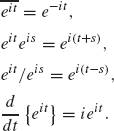
The next lemma shows that the familiar properties of the real exponential also hold for the complex exponential. These properties follow from the definition together with basic trigonometric identities and will be left to the exercises (see exercise 16).
Lemma 1.16 For all t, s ∈ R, we have

The next theorem shows that the complex exponentials are orthonormal in L2([π, π}).
Theorem 1.17 The set of functions ![]() is orthonormal in L2([–π, π]).
is orthonormal in L2([–π, π]).
Proof. We must show
![]()
Using the third, fourth, and sixth properties in Lemma 1.16, we have
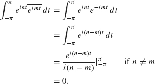
If n = m, then einte –int = 1 and so 〈eint, eint〉 = 2π. This completes the proof.
Combining this theorem with Theorem 0.21, we obtain the following complex version of Fourier series.
Theorem 1.18 If ![]() on the interval –π ≤ t ≤ π, then
on the interval –π ≤ t ≤ π, then
![]()
Example 1.19 Consider the function
![]()
The nth complex Fourier coefficient is
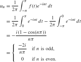
So the complex Fourier series of f is
![]()
The complex form of Fourier series can be formulated on other intervals as well.
Theorem 1.20 The set of functions
![]()
is an orthonormal basis for L2[–a, a]. If ![]() , then
, then
![]()
Relation Between the Real and Complex Fourier Series. If f is a real-valued function, the real form of its Fourier series can be derived from its complex form and vice-versa. For simplicity, we discuss this derivation on the interval –π ≤ t ≤ π, but this discussion also holds for other intervals as well. We first decompose the complex form of the Fourier series of f into positive and negative terms:
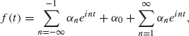
where
![]()
If f is real-valued, then ![]() because
because
![]()
Therefore, Eq. (1.21) becomes
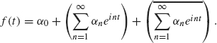
Since ![]() for any complex number z, this equation can be written as
for any complex number z, this equation can be written as
Now note the following relations between αn and the real Fourier coefficients, an and bn given in Theorem 1.2:
Using Eq. (1.22), we obtain
which is the real form of the Fourier series of f. These equations can also be stated in reverse order so that the complex form of its Fourier series can be derived from its real Fourier series.
1.3 CONVERGENCE THEOREMS FOR FOURIER SERIES
In this section, we prove the convergence of Fourier series under mild assumptions on the original function f. The mathematics underlying convergence is somewhat involved. We start with the Riemann-Lebesgue Lemma, which is important in its own right.
1.3.1 The Riemann-Lebesgue Lemma
In the examples in Section 1.2.4, the Fourier coefficients ak and bk converge to zero as k gets large. This is not a coincidence as the following theorem shows.
Theorem 1.21 Riemann-Lebesgue Lemma. Suppose f is a piecewise continuous function on the interval a ≤ x ≤ b. Then
![]()
A function is piecewise continuous if on any closed, bounded interval it has only a finite number of discontinuities, all of which are “jumps,” where the left-hand and right-hand limits exist but are not equal (cf. Section 1.3.3). For example, the function shown in Figure 1.10 is piecewise continuous: It has only jump discontinuities at the points x = 0, ±1, ±2,..., but it is otherwise continuous. The hypothesis that f is piecewise continuous sufficient for our needs here, but it can be weakened considerably.
One important consequence of Theorem 1.21 is that only a finite number of Fourier coefficients are larger (in absolute value) than any given positive number. This fact is the basic idea underlying the process of data compression. One way to compress a signal is first to express it as a Fourier series and then discard all the small Fourier coefficients and retain (or transmit) only the finite number of Fourier coefficients that are larger than some given threshold. (See exercise 35 for an illustration of this process.) We encounter data compression again in future sections on the discrete Fourier transform and wavelets.
Proof. The intuitive idea behind the proof is that as k gets large, sin(kx) and cos(kx) oscillate much more rapidly than does f (see Figure 1.13). If k is large, f(x) is nearly constant on two adjacent periods of sin kx or cos kx. The graph of the product of f(x) with sin(kx) is given in Figure 1.14 (the graph of the product of f with coskx is similar). The integral over each period is almost zero, since the areas above and below the x axis almost cancel.
We give the following analytical proof of the theorem in the case of a continuously differentiable function f. Consider the term
![]()
Fig. 1.13. Plot of both y = f(x) and y = sinkx.
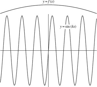
Fig. 1.14. Plot of y = f(x) sinkx.
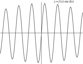
We integrate by parts with u = f and dv = coskx to obtain
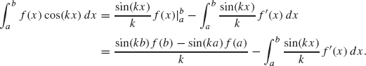
As k gets large in the denominator, the expression on the right converges to zero, and this completes the proof.
1.3.2 Convergence at a Point of Continuity
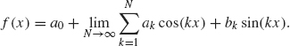
The sum appearing in a Fourier expansion generally contains an infinite number of terms (the Fourier expansions of Examples 1.11 and 1.12 are exceptions). An infinite sum is, by definition, a limit of partial sums, that is,
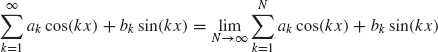
provided the limit exists. Therefore, we say that the Fourier series of f converges to f at the point x if
With this in mind, we state and prove our first theorem on the convergence of Fourier series.
Theorem 1.22 Suppose f is a continuous and 2π-periodic function. Then for each point x, where the derivative of f is defined, the Fourier series of f at x converges to f(x).
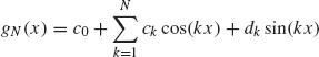
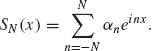
Proof. For a positive integer N, let
where ak and bk are the Fourier coefficients of the given function f. Our ultimate goal is to show SN(x) → f(x) as N → ∞. Before this can be done, we need to rewrite SN into a different form. This process requires several steps.
Step 1. Substituting the Fourier Coefficients. After substituting the formulas for the ak and bk (1.12)–(1.14), we obtain
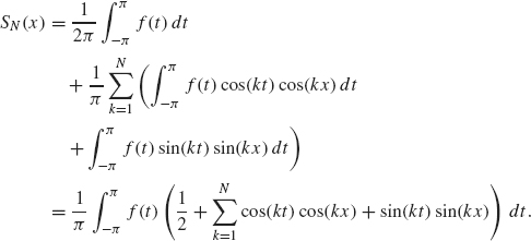
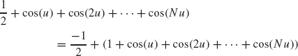
Using the addition formula for the cosine function, cos(A – B) = cos(A) cos(B) + sin(A) sin(B), we obtain
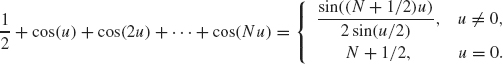
To evaluate the sum on the right side, we need the following lemma.
Step 2. Evaluating the Sum on the Right Side.
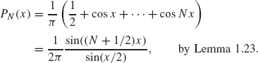
Lemma 1.23 For any number u, –π ≤ u ≤ π,
Proof of Lemma 1.23. Recall the complex exponential is defined as eiu = cos(u) + i sin(u). Note that
![]()
So, cos nu = Re{(eiu)n}. Therefore
and so
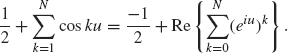
The sum on the right is a geometric series, ![]() , where z = eiu.
, where z = eiu.
For any number z, we have
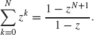
This formula is established as follows: let

Then
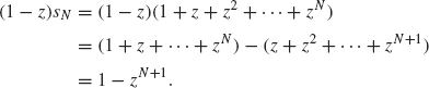
Dividing both sides by (1 – z) yields Eq. (1.26).
Applying (1.26) with z = eiu to (1.25), we obtain
To compute the expression on the right, we multiply the numerator and denominator by e–u/2:
![]()
The denominator on the right is –2i sin(u/2); so
![]()
Inserting this equation into the right side of Eq. (1.27) gives
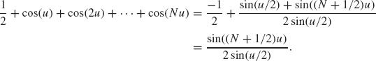
This completes the proof of Lemma 1.23.
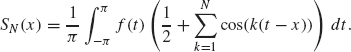
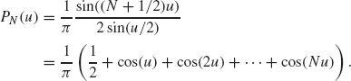
Step 3. Evaluation of the Partial Sum of Fourier Series. Using Lemma 1.23 with u = t – x, Eq. (1.24) becomes
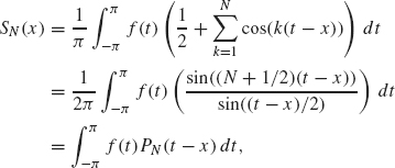
where we have let
Now use the change of variables u = t – x in the preceding integral to obtain
![]()
Since both f and PN are periodic with period 2π, the limits of integration can be shifted by x without changing the value of the integral (see Lemma 1.3). Therefore
Next, we need the following lemma.
Step 4. Integrating the Fourier Kernel.
Lemma 1.24
![]()
Proof of Lemma 1.24. We use Lemma 1.23 to write
Integrating this equation gives
![]()
The second integral on the right is zero (since the antiderivatives involve the sine, which vanishes at multiples of π). The first integral on the right is one, and the proof of the lemma is complete.
Step 5. The End of the Proof of Theorem 1.22. As indicated at the beginning of the proof, we must show that SN(x) → f(x) as N → ∞. Inserting the expression for SN(x) given in Eq. (1.29), we must show
In view of Lemma 1.24, ![]() and so we are reduced to showing
and so we are reduced to showing
![]()
Using Eq. (1.28), the preceding limit becomes
We can use the Riemann-Lebesgue Lemma (see Theorem 1.21) to establish Eq. (1.31), provided that we show that the function
![]()
is continuous (as required by the Riemann-Lebesgue Lemma). Here, x is a fixed point and u is the variable. The only possible value of u ∈ [–π, π] where g(u) could be discontinuous is u = 0. However, since ![]() exists by hypothesis, we have
exists by hypothesis, we have
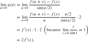
Thus g(u) extends across u = 0 as a continuous function by defining g(0) = 2f’(x). We conclude that Eq. (1.31) holds by the Riemann-Lebesgue Lemma. This finishes the proof of Theorem 1.22.
Fig. 1.15. Periodic extension of f(x) = x.
1.3.3 Convergence at a Point of Discontinuity
Now we discuss some variations of Theorem 1.22. Note that the hypothesis of this theorem requires the function f to be continuous and periodic. However, there are many functions of interest that are neither continuous or periodic. For example, the function in Example 1.9, f(x) = x is not periodic. Moreover, the periodic extension of f (graphed in Figure 1.15) is not continuous.
Before we state the theorem on convergence near a discontinuity, we need the following definition.
Definition 1.25 The right and left limits of f at a point x are defined as follows:
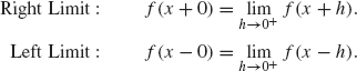
The function f is said to be right differentiable if the following limit exists:
![]()
The function f is said to be left differentiable if the following limit exists:
![]()
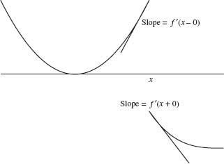
Intuitively, f’(x – 0) represents the slope of the tangent line to f at x considering only the part of the graph of y = f(t) that lies to the left of t = x. The value f’(x + 0) is the slope of the tangent line of y = f(t) at x considering only the graph of the function that lies to the right of t = x (see Figure 1.16). These can exist even when f itself is discontinuous, for example when it has a jump discontinuity, which, in Section 1.3.1, we defined to be a point x for which f(x + 0) and f(x – 0) both exist, but f(x + 0) ≠ f(x – 0).
Fig. 1.16. Left and right derivatives.
Example 1.26 Let f(x) be the periodic extension of y = x, –π ≤ x ≤ π. Then f(x) is discontinuous at x = ..., –π, π, .... The left and right limits of f at x = π are
![]()
The left and right derivatives at x = π are
![]()
Example 1.27 Let
![]()
The graph of f is the sawtooth wave illustrated in Figure 1.7. This function is continuous, but not differentiable at x = π/2. The left and right derivatives at x = π/2 are
![]()
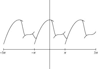
Fig. 1.17. Graph of the Fourier series for Example 1.29.
Now we are ready to state the convergence theorem for Fourier series at a point where f is not necessarily continuous.
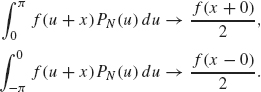
Theorem 1.28 Suppose f(x) is periodic and piecewise continuous. Suppose x is a point where f is left and right differentiable (but not necessarily continuous). Then the Fourier series of f at x converges to
![]()
This theorem states that at a point of discontinuity of f, the Fourier series of f converges to the average of the left and right limits of f. At a point of continuity, the left and right limits are the same and so in this case, Theorem 1.28 reduces to Theorem 1.22.
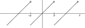
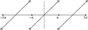
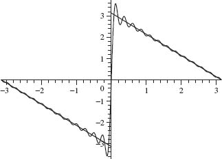
Example 1.29 Let f(x) be the periodic extension of y = x, –π ≤ x ≤ π. As mentioned in Example 1.26, f is not continuous, but left and right differentiable at x = π. Theorem 1.28 states that its Fourier series, F(x), converges to the average of the left and right limits of f at x = π. Since f(π – 0) = π and f(π + 0) = –π, Theorem 1.28 implies F(π) = 0. This value agrees with the formula for the Fourier series computed in Example 1.9:
![]()
whose value is zero at x = π. The graph of F is given in Figure 1.17. Note that the value of F at x = ±π and x = ±3π (indicated by the solid dots) is equal to the average of the left and right limits at x = ±π and x = ±3π.
Proof of Theorem 1.28. The proof of this theorem is very similar to the proof of Theorem 1.22. We summarize the modifications.
Steps 1 through 3 go through without change. Step 4 needs to be modified as follows:
Step 4’.
![]()
where
![]()
In fact, these equalities follow from Lemma 1.24 and by using the fact that PN(u) is even (so the left and right half-integrals are equal and sum to 1).
Step 5 is now replaced by the following.
Step 5’. To show Theorem 1.28, we need to establish
as N → ∞.
We show Eq. (1.32) by establishing the following two limits:
Using Step 4’, these limits are equivalent to the following two limits:
Using the definition of PN(u), Eq. (1.33) is equivalent to showing
![]()
This limit follows from the Riemann-Lebesgue Lemma exactly as in Step 5. Since u is positive in the preceding integral, we only need to know that the expression in parentheses is continuous from the right (i.e., has a right limit as u → 0+). Since f is assumed to be right differentiable, the same limit argument from Step 5 can be repeated here (with u > 0).
Similar arguments can be used to establish Eq. (1.34). This completes the proof of Theorem 1.28.
1.3.4 Uniform Convergence
Now we discuss uniform convergence of Fourier series. As stated in Definition 0.8, a sequence of functions Fn(x) converges uniformly to F(x) if the rate of convergence is independent of the point x. In other words, given any small tolerance, ∈ > 0 (such as ∈ = .01), there exists a number N that is independent of x, such that |Fn(x) – F(x)| < ∈ for all x and all n ≥ N. If the FN did not converge uniformly, then one might have to choose different values of N for different x values to achieve the same degree of accuracy.
We say that the Fourier series of f(x) converges to f(x) uniformly if the sequence of partial sums
converges to f(x) uniformly as N → ∞, where the ak and bk are the Fourier coefficients of f.
From Figures 1.8 and 1.9, it appears that the Fourier series in Example 1.10 converges uniformly. By contrast, the Fourier series in Example 1.9 does not appear to converge uniformly to f(x). As the point x gets closer to a point of discontinuity of f, the rate of convergence gets slower. Indeed, the number of terms, N, that must be used in the partial sum of the Fourier series to achieve a certain degree of accuracy must increase as x approaches a point of discontinuity.
In order to state the following theorem on uniform convergence, one more definition is needed. A function is said to be piecewise smooth if it is piecewise continuous and its first derivative is also piecewise continuous. On any closed, bounded interval, a piecewise smooth function can have a finite number jump discontinuities and corners, where its left and right derivatives exist but may not be equal. Except for these points, f is continuously differentiable. For example, the 2π-periodic extension of f(x) = x, –π ≤ x < π, shown in Figure 1.4, has jump discontinuities at multiples of π, and so does its derivative. Otherwise, it is continuously differentiable. For us, a more important instance is the sawtooth function in Example 1.10. This function is both continuous mdpiecewise smooth. The derivatives involved exist at all points except at multiples of π/2, where the sawtooth function has corners, which are just jump discontinuities in its derivative.
We now state the theorem for uniform convergence of Fourier series for the interval [–π, π]. This theorem also holds with π replaced by any number a.
Theorem 1.30 The Fourier series of a continuous, piecewise smooth 2π -periodic function f(x) converges uniformly to f(x) on [–π, π].
Example 1.31 Consider the sawtooth wave in Example 1.10. The graph of its periodic extension is piecewise smooth, as is clear from Figure 1.7. Therefore, Theorem 1.30 guarantees that its Fourier series converges uniformly.
Example 1.32 Consider the Fourier series for the function f(x) = x on the interval [–π, π] considered in Example 1.9. Since f(x) = x is not periodic, we need to consider its periodic extension, which is graphed in Figure 1.4. Note that although its periodic extension is piecewise smooth, it is not continuous–even though f(x) = x is everywhere smooth. Therefore, Theorem 1.30 does not apply. In fact, due to the Gibbs effect in this example (see Figures 1.5 and 1.6), the Fourier series for this example does not converge uniformly.
Proof of Theorem 1.30. We prove this theorem under the simplifying assumption that f is everywhere twice differentiable.
As a first step, we prove the following relationship between the Fourier coefficients of f and the corresponding Fourier coefficients of f”: If
then
To establish the first relation, we use integration by parts on the integral formula for an (Theorem 1.2) to obtain
The first term on the right is zero since sin nπ = sin(– nπ) = 0. The second term on the right is ![]() , where
, where ![]() is the Fourier sine coefficient of f’. Repeating the same process (this time with dv = (sin nx)/n and u = f’) gives
is the Fourier sine coefficient of f’. Repeating the same process (this time with dv = (sin nx)/n and u = f’) gives
![]()
The right side is ![]() , as claimed in (1.35). Equation (1.36) for bn is proved in a similar manner.
, as claimed in (1.35). Equation (1.36) for bn is proved in a similar manner.
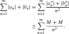
If f” is continuous, then both the ![]() and
and ![]() stay bounded by some number M (in fact, by the Riemann-Lebesgue Lemma,
stay bounded by some number M (in fact, by the Riemann-Lebesgue Lemma, ![]() and
and ![]() converge to zero as n → ∞). Therefore using (1.35) and (1.36), we obtain
converge to zero as n → ∞). Therefore using (1.35) and (1.36), we obtain
This series is finite by the integral test for series (i.e., ![]() is finite since
is finite since ![]() is finite).
is finite).
The proof of the theorem will now follow from the following lemma.
Lemma 1.33 Suppose
![]()
with
![]()
Then the Fourier series converges uniformly and absolutely to the function f(x).
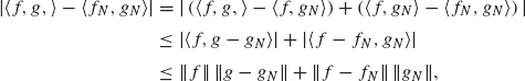
Proof. We start with the estimate
(valid since |cos t|, |sin t ≤ 1). Thus the rate of convergence of the Fourier series of f at any point x is governed by the rate of convergence of ![]() . More precisely, let
. More precisely, let
Then
The a0 and the terms up through k = N cancel. Thus
![]()
By Eq. (1.37), we have
uniformly for all x. Since the series ![]() converges by hypothesis, the tail end of this series can be made as small as desired by choosing N large enough. So given ∈ > 0, there is an integer N0 > 0 so that if N > N0, then
converges by hypothesis, the tail end of this series can be made as small as desired by choosing N large enough. So given ∈ > 0, there is an integer N0 > 0 so that if N > N0, then ![]()
![]() . From Eq. (1.38), we have
. From Eq. (1.38), we have
![]()
for all x. N does not depend on x; N depends only on the rate of convergence of ![]() . Therefore, the convergence of SN(x) is uniform. This completes the proof of Lemma 1.33 and of Theorem 1.30.
. Therefore, the convergence of SN(x) is uniform. This completes the proof of Lemma 1.33 and of Theorem 1.30.
1.3.5 Convergence in the Mean
As pointed out in the previous section, if f(x) is not continuous, then its Fourier series does not converge to f(x) at points where f(x) is discontinuous (it converges to the average of its left and right limits instead). In cases where a Fourier series does not converge uniformly, it may converge in a weaker sense, such as in L2 (in the mean). We investigate L2 convergence of Fourier series in this section. Again, we state and prove the results in this section for 2π-periodic functions. However, the results remain true for other intervals as well (by replacing π by any number a and by using the appropriate form of the Fourier series for the interval [–a, a]).
First, we recall some concepts from Chapter 0 on inner product spaces. We will be working with the space V = L2([–π, π) consisting of all square integrable functions (i.e., f with ![]() ). V is an inner product space with the following inner product:
). V is an inner product space with the following inner product:
![]()
The norm ||f|| in this space is therefore defined by
![]()
We remind you of the two most important inequalities of an inner product space:
![]()
The first of these is the Schwarz inequality and the second is the triangle inequality.
Let
![]()
An element in VN is a sum of the form
where ck and dk are any complex numbers. Suppose f belongs to L2[–π, π]. Let
be its partial Fourier series, where the ak and bk are the Fourier coefficients given in Theorem 1.2. The key point in the proof of Theorem 1.2 is that ak and bk are obtained by orthogonally projecting f onto the space spanned by cos(kx) and sin(kx) (see the remark just after Theorem 1.2). Thus, fN is the orthogonal projection of f onto the space VN. In particular, fN is the element in VN that is closest to f in the L2 sense. We summarize this discussion in the following lemma.
Lemma 1.34 Suppose f is an element of V = L2([–π, π]). Let
![]()
Let
where ak and bk are the Fourier coefficients of f. Then fN is the element in VN which is the closest to f in the L2 norm, that is,
![]()
The main result of this section is contained in the next theorem.
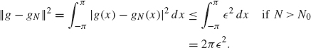
Theorem 1.35 Suppose f is an element of L2([–π, π]). Let

where ak and bk are the Fourier coefficients of f. Then fN converges to f in L2([π, π]), that is, ||fN – f||L2→ 0 as N → ∞.
Theorem 1.35 also holds for the complex form of Fourier series.
Theorem 1.36 Suppose f is an element of L2([–π, π]) with (complex) Fourier coefficients given by
![]()
Then the partial sum
converges to f in the L2([–π, π]) norm as N → ∞.
Example 1.37 All the examples considered in this chapter arise from functions that are in L2 (over the appropriate interval under consideration for each example). Therefore, the Fourier series of each example in this chapter converges in the mean.
Proof. The proofs of both theorems are very similar. We will give the proof of Theorem 1.35.
The proof of this involves two key steps. The first step (the next lemma) states that any function in L2([–π, π) can be approximated in the L2 norm by a piecewise smooth periodic function g. The second step (Theorem 1.30) is to approximate g uniformly (and therefore in L2) by its Fourier series. We start with the following lemma.
Lemma 1.38 A function in L2([–π, π]) can be approximated arbitrarily closely by a smooth, 2π-periodic function.
A rigorous proof of this lemma is beyond the scope of this book. However, we can give an intuitive idea as to why this lemma holds. A typical element f ∈ L2[–π, π] is not continuous. Even if it were continuous, its periodic extension is often not continuous. The idea is to connect the continuous components of f with the graph of a smooth function g. This is illustrated in Figures 1.18-1.20. In Figure 1.18, the graph of a typical f ∈ L2[–π, π] is given. The graph of its periodic extension is given in Figure 1.19. In Figure 1.20, the graph of a continuous g that connects the continuous components of f is superimposed on the graph of f. Rounding the corners of the connecting segments then molds g into a smooth function. Since the extended f is periodic, we can arrange that g is periodic as well.
The graph of g agrees with the graph of f everywhere except on the connecting segments that connect the continuous components of f. Since the horizontal width of each of these segments can be made very small (by increasing the slopes of these connecting segments), g can be chosen very close to f in the L2 norm. These ideas are explored in more detail in Exercise 31.
Now we can complete the proof of Theorem 1.36. Suppose f ∈ L2[–π, π]. Using Lemma 1.38, we can (for any ∈ > 0) choose a differentiable periodic function g with
Fig. 1.18. Typical f in L2.
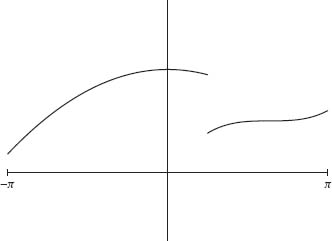
Fig. 1.19. Periodic extension of f.
Let
where ck and dk are the Fourier cosine and sine coefficients for g. Since g is differentiable and periodic, we can uniformly approximate g by gN using Theorem 1.30. By choosing N0 large enough, we can arrange |g(x) – gN(x)| < ∈
Fig. 1.20. Approximation of f by a smooth g.
for all x ∈ [–π, π] and for N > N0. We have
By taking square roots, we obtain
![]()
Combining this estimate with (1.39), we obtain
![]()
Now gN is a linear combination of sin(kx) and cos(kx) for k ∈ N and therefore gN belongs to VN. We have already shown that fN is the closest element from VN to f in the L2 norm (see Lemma 1.34). Therefore, we conclude
![]()
Since the tolerance, ∈, can be chosen as small as desired, the proof of Theorem 1.35 is complete.
One consequence of Theorems 1.35 and 1.36 is the following theorem, which is known as Parseval’s equation. We will state both the real and complex versions.
Theorem 1.39 Parseval’s Equation—Real Version. Suppose
![]()
Then
Theorem 1.40 Parseval’s Equation—Complex Version. Suppose
![]()
Then
Moreover, for f and g in L2[–π, π] we obtain
Remark. The L2 norm of a signal is often interpreted as its energy. With this physical interpretation, the squares of the Fourier coefficients of a signal measure the energy of the corresponding frequency components. Therefore, a physical interpretation of Parseval’s equation is that the energy of a signal is simply the sum of the energies from each of its frequency components. (See Example 1.41.)
Proof. We prove the complex version of Parseval’s equation. The proof of the real version is similar.
We prove Eq. (1.42). Equation (1.41) then follows from Eq. (1.42) by setting f = g.
Let
be the partial sum of the Fourier series of f and g, respectively. By Theorem 1.36 , fN → f and gN → g in L2[–π, π] as N → ∞. We have
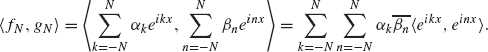
Since ![]() is orthonormal, 〈eikx, einx〉 is 0 if k ≠ n and 2π if k = n. Therefore
is orthonormal, 〈eikx, einx〉 is 0 if k ≠ n and 2π if k = n. Therefore
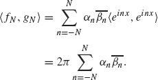
Equation (1.42) follows by letting N → ∞, provided that we show
To show (1.43), we write
where the last step follows by Schwarz’s Inequality. Since ||fN – f|| → 0 and ||g – gN|| → 0 in L2, the right side converges to zero as N → ∞ and Eq. (1.43) follows.
Note. If the series on the right side of Eq. (1.41) is truncated at some finite value N, then the right side can only get smaller, resulting in the following inequality:
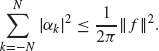
This in known as Bes sel’s Inequality.
Example 1.41 As we noted earlier, one interpretation of Parseval’s Theorem is that the energy in a signal is the sum of the energies associated with its Fourier components. In Example 1.9, we found that the Fourier coefficients for f(x) = x, –π ≤ x < π are an = 0 and bn = (2/n)(–1)n+1. By Eq. (1.40), we have
![]()
Evaluating the integral on the left and dividing both sides by 4, we see that
![]()
This sum is computed another way in Exercise 22.
1. Expand the function f(x) = x2 in a Fourier series valid on the interval –π ≤ x ≤ π. Plot both f and the partial sums of its Fourier series,
for N = 1, 2, 5, 7. Observe how the graphs of the partial sums SN(x) approximate the graph of f. Plot the same graphs over the interval –2π ≤ x ≤ 2π.
2. Repeat the previous exercise for the interval –1 ≤ x ≤ 1. That is, expand the function f(x) = x2 in a Fourier series valid on the interval –1 ≤ x ≤ 1. Plot both f and the partial Fourier series
for N = 1, 2, 5, 7 over the interval –1 ≤ x ≤ 1 and –2 ≤ x ≤ 2.
3. Expand the function f(x) = x2 in a Fourier cosine series on the interval 0 ≤ x ≤ π.
4. Expand the function f(x) = x2 in a Fourier sine series on the interval 0 ≤ x ≤ 1.
5. Expand the function f(x) = x3 in a Fourier cosine series on the interval 0 ≤ x ≤ π.
6. Expand the function f(x) = x3 in a Fourier sine series on the interval 0 ≤ x ≤ 1.
7. Expand the function f (x) = |sin x| in a Fourier series valid on the interval –π ≤ x ≤ π.
8. Expand the function
![]()
in a Fourier series valid on the interval –1 ≤ x ≤ 1. Plot the various partial Fourier series along with the graph of f as in exercise 1 for N = 5, 10, 20, and 40 terms. Notice how much slower the series converges to f in this example than in exercise 1. What accounts for the slow rate of convergence in this example?
9. Expand the function f(x)= cos x in a Fourier sine series on the interval 0 ≤ x ≤ π.
10. Consider the function f(x) = π – x, 0 ≤ x ≤ π.
(a) Sketch the even, 2π-periodic extension of f. Find the Fourier cosine series for f.
(b) Sketch the odd, 2π-periodic extension of f. Find the Fourier sine series for.
(c) Sketch the π-periodic extension of f. Find the Fourier series for f.
11. Let f(x) = e–x/3, –π ≤ π and let g(x) = e–x/3, but now defined on 0 ≤ x ≤ 2π.
(a) Plot the 2π-periodic extension of f. Find the complex form of the Fourier series for f.
(b) Plot the 2π-periodic extension of g. Find the complex form of the Fourier series for g. (Hint: Use Lemma 1.3 in connection with finding the complex coefficients.)
12. Expand the function f(x) = erx in a Fourier series valid for –π ≤ x ≤ π. For the case r = 1/2, plot the partial Fourier series along with the graph of f as in problem 1 for N = 10, 20 and 30 terms. Plot these functions over the interval –π ≤ x ≤ π and also –2π ≤ x ≤ 2π.
13. Use Exercise 12 to compute the Fourier coefficients for the function f(x) = sinh x = (ex – e–x)/2 and f(x) = cosh(x) = (ex + e–x)/2 over the interval –π ≤ x ≤ π.
14. Show that
![]()
15. Show that
is an orthonormal set of functions in the space L2([–a, a]). Establish the proof of Theorem 1.4.
16. Prove Lemma 1.16 and Theorem 1.20.
17. Let SN(x) be the real form of the partial sum defined in Eq. (1.23). Show that if the complex form of the Fourier series is used instead, then SN also can be expressed as
18. Let f and g be 2π-periodic, piece wise smooth functions having Fourier series ![]() and
and ![]() , and define the convolution of f and g to be
, and define the convolution of f and g to be ![]() . Show that the complex form of the Fourier series for f * g is
. Show that the complex form of the Fourier series for f * g is
![]()
19. Let F(x) be the Fourier series for the function
![]()
State the precise value of F(x) for each x in the interval –1 ≤ x ≤ 1.
20. If f(x) is continuous on the interval 0 ≤ x ≤ a, show that its even periodic extension is continuous everywhere. Does this statement hold for the odd periodic extension? What additional condition(s) is (are) necessary to ensure that the odd periodic extension is everywhere continuous?
21. Consider the sawtooth function and the Fourier series derived for it Example 1.10.
(a) Use the convergence theorems in this chapter to explain why the Fourier series for the sawtooth function converges pointwise to that function.
(b) Use this fact to show that
![]()
22. In exercise 1, you found the Fourier series for the function f(x) = x2, –π ≤ x ≤ π. Explain why this series converges uniformly to x2 on [–π, π]. Use this to show that ![]() . (Hint: What happens at x = π?)
. (Hint: What happens at x = π?)
23. Sketch two periods of the pointwise limit of the Fourier series for each of the following functions. State whether or not each function’s Fourier series converges uniformly. (You do not need to compute the Fourier coefficients.)
(a) f(x) = ex, –1 < x ≤ 1
(b) ![]()
(c) f(x) = x – x2, –1 < x ≤ 1
(d) f(x) = 1 – x2, –1 < x ≤ 1
(e) f(x) = cos x + |cos x|, –π < x ≤ π
(f) ![]()
24. For each of the functions in exercise 23, state whether or not its Fourier sine and cosine series (for the corresponding half-interval) converge uniformly on the entire real line, –∞ < x < ∞.
25. If F is a 2π-periodic and c is any real number, then show that
![]()
Then use this equation to prove Lemma 1.3. Hint: Use the change of variables x = t – 2π.
26. If f is a real-valued even function on the interval [–π, π], show that the complex Fourier coefficients are real. If f is a real-valued odd function on the interval [–π, π], show that the complex Fourier coefficients are purely imaginary (i.e., their real parts are zero).
27. Suppose f is continuously differentiable (i.e., f’(x) is continuous for all x) and 2π-periodic. Without quoting Theorem 1.35, show that the Fourier series of f converges in the mean. Hint: Use the relationship between the Fourier coefficients of f and those of f’ given in the proof of Theorem 1.30.
28. From Theorem 1.8, the Fourier series of an odd function consists only of sine terms. What additional symmetry conditions on f will imply that the sine coefficients with even indices will be zero? Give an example of a function satisfying this additional condition?
29. Suppose that there is a sequence of nonnegative numbers {Mn} such that ![]() is convergent and that
is convergent and that
![]()
Show that the following series is uniformly convergent on –∞ < x < ∞.
![]()
30. Prove the following version of the Riemann-Lebesgue Lemma for infinite intervals: Suppose f is a continuous function on a ≤ t < ∞ with ![]() show that
show that
![]()
Hint: break up the interval a ≤ t ≤ ∞ into two intervals: a ≤ t ≤ M and M ≤ t ≤ ∞ where M is chosen so large that ![]() is less than ∈/2; apply the usual Riemann-Lebesgue Lemma to the first interval.
is less than ∈/2; apply the usual Riemann-Lebesgue Lemma to the first interval.
31. This exercise explores the ideas in the proof of Lemma 1.38 with a specific function. Let
![]()
For 0 < δ < 1/2, let
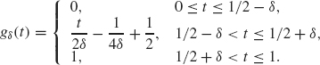
Graph both f and gδ for δ = 0.1 Show that as δ ![]() 0, ||f – gδ|| L2[0, 1] → 0. Note that gδ is continuous but not differentiable. Can you modify the formula for gδ so that gδ is C1 (one continuous derivative) and still satisfy
0, ||f – gδ|| L2[0, 1] → 0. Note that gδ is continuous but not differentiable. Can you modify the formula for gδ so that gδ is C1 (one continuous derivative) and still satisfy ![]()
32. This exercise explains the Gibbs phenomenon that is evident in the convergence of Fourier series near a point of discontinuity. We examine the Gibbs phenomenon for the Fourier series of the function
![]()
on the interval –π ≤ x ≤ π (see Figure 1.21 for the graph of f and its partial Fourier series). Complete the following outline.
(a) Show that the Fourier series for f is
![]()
(b) Let
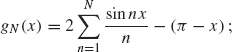
gN represents the difference between the f(x) and the Nth partial sum of the Fourier series of f. In the remaining parts of this problem, you will show that the maximum value of gN is greater than 0.5 when N is large and thus represents the Gibbs effect.
Fig. 1.21. Gibbs phenomenon.
(c) Show that ![]() , where
, where
(d) Show that θN = π/(N + 1/2) is the first critical point of gN to the right of x = 0.
(e) Use the Fundamental Theorem of Calculus and part c to show
![]()
(f) Show
![]()
Hint: Make a change of variables ϕ = (N + 1/2)x and use the fact that sin t/t → 1 as t → 0.
(g) Show that
![]()
by evaluating this integral numerically. Thus the Gibbs effect or the amount that the Nth partial sum overshoots the function f is about 0.562 when N is large.
33. Use Parseval’s Theorem and the series from exercise 1 to find the sum of the series ![]() .
.
The next two problems require a computer algebra system (e.g., Maple or MATLAB) to compute Fourier coefficients.
34. Consider the function
![]()
For what values of n would you expect the Fourier coefficients a(n) and b(n) to be significant (say bigger than 0.01 in absolute value)? Why? Compute the a(n) and b(n) through n = 50 and see if you are right. Plot the partial Fourier series through n = 6 and compare with the plot of the original f(x).
35. Consider the function
![]()
Compute the partial Fourier series through N = 25. Throw away any coefficients that are smaller than .01 in absolute value. Plot the resulting series and compare with the original function g(x). Try experimenting with different tolerances (other than .01).
The remaining exercises pertain to Fourier series as a tool for solving partial differential equations, as indicated at the beginning of this chapter.
36. Solve the following heat equation problem:
37. If the boundary conditions u(0, t) = A and u(1, t) = B are not homogeneous (i.e., A and B are not necessarily zero), then the procedure given in Section 1.1.3 for solving the heat equation
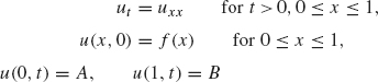
must be modified. Let L(x) be the linear function with L(0) = A and L(1) = B and let û(x, t) = u(x, t) – L(x). Show that û solves the following problem:
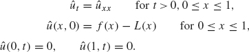
This heat equation can be solved for û using the techniques given in Section 1.1.3. The solution, u, to the original heat equation problem can then be found by the equation u(x, t) = û(x, t) + L(x).
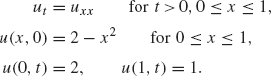
38. Use the procedure outlined in the previous exercise to solve the following heat equation:
39. Another important version of the heat equation is the following Neumann boundary value problem:
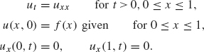
This problem represents the standard heat equation where u(x,t) is the temperature of a rod of unit length at position x and at time t; f(x) is the initial (at time t = 0) temperature at position x. The boundary conditions ux = 0 at x = 0 and x = 1, physically means that no heat is escaping from the rod at its endpoints (i.e., the rod is insulated at its endpoints). Use the procedure outlined at the beginning of this chapter to show that the general solution to this problem is given by
![]()
where ak are the coefficients of a Fourier cosine series of f over the interval 0 ≤ x ≤ 1. Use this formula to obtain the solution in the case where f(x) = x2 – x for 0 ≤ x ≤ 1.
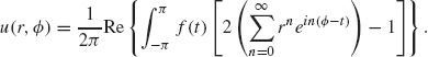
40. The goal of this problem is to prove Poisson’s formula which states that if f(t) is a piecewise smooth function on –π ≤ t ≤ πthen
for 0 ≤ r ≤ 1, 0 ≤ ϕ ≤ 2π solves Laplace’s equation
in the unit disc x2 + y2 ≤ 1 (in polar coordinates: {r ≤ 1}) with boundary values u (r = 1, ϕ) = f(ϕ) –π ≤ ϕ ≤ π Follow the outline given to establish this formula.
(a) Show that the functions u(x, y) = (x + iy)n and u(x, y) = (x – iy)n both solve Laplace’s equation for each value of n = 0,1, 2, Using complex notation z = x + iy, these solutions can be written as u(z) = zn and ![]()
(b) Show that any finite sum of the form ![]() where An and A–n are real (or complex) numbers solves Laplace’s equation. It is a fact that if the infinite series (i.e., as |N| → ∞) converges uniformly and absolutely for |z| = 1, then the infinite series
where An and A–n are real (or complex) numbers solves Laplace’s equation. It is a fact that if the infinite series (i.e., as |N| → ∞) converges uniformly and absolutely for |z| = 1, then the infinite series ![]() also solves Laplace’s equation inside the unit circle |z| = 1. Write this function in polar coordinates with z = reiϕ and show that we can express it as
also solves Laplace’s equation inside the unit circle |z| = 1. Write this function in polar coordinates with z = reiϕ and show that we can express it as ![]() .
.
(c) In order to solve Laplace’s equation, we therefore must hunt for a solution of the form ![]() with boundary condition u(r = 1, ϕ) = f(ϕ). Show the boundary condition is satisfied if An is set to the Fourier coefficients of f in complex form.
with boundary condition u(r = 1, ϕ) = f(ϕ). Show the boundary condition is satisfied if An is set to the Fourier coefficients of f in complex form.
(d) Using the formula for the complex Fourier coefficients, show that if f is real-valued, then ![]() . Use this fact to rewrite the solution in the previous step as
. Use this fact to rewrite the solution in the previous step as
(e) Now use the geometric series formula to rewrite the solution in the previous step as
![]()
where
![]()
(f) Rewrite P as
![]()
Use this formula together with the previous integral formula for u to establish Eq. (1.44).