2
THE FOURIER TRANSFORM
In this section, we develop the Fourier transform and its inverse. The Fourier transform can be thought of as a continuous form of Fourier series. A Fourier series decomposes a signal on [–π, π] into components that vibrate at integer frequencies. By contrast, the Fourier transform decomposes a signal defined on an infinite time interval into a λ-frequency component where λ can be any real (or even complex) number. Besides being of interest in their own right, the topics in this chapter will be important in the construction of wavelets in the later chapters.
2.1 INFORMAL DEVELOPMENT OF THE FOURIER TRANSFORM
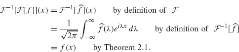
2.1.1 The Fourier Inversion Theorem
In this section we give an informal development of the Fourier transform and its inverse. Precise arguments are given in the Appendix (see A.l).
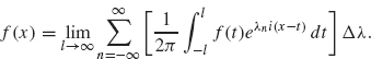
To obtain the Fourier transform, we consider the Fourier series of a function defined on the interval –l ≤ x ≤ l and then let l go to infinity. Recall from Theorem 1.20 (with a = l) that a function defined on –l ≤ x ≤ l can be expressed as
where
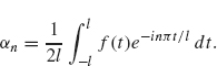
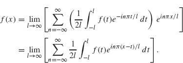
If f is defined on the entire real line, then it is tempting to let l go to infinity and see how the preceding formulas are affected. Substituting the expression for αn into the previous sum, we obtain
Our goal is to recognize the sum on the right as the Riemann sum formulation of an integral. To this end, let ![]() . We obtain
. We obtain
Let
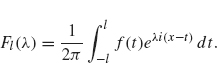
The sum in Eq. (2.1) is
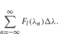
This term resembles the Riemann sum definition of the integral ![]() .As l converges to ∞, the quantity Δλ. converges to 0 and so Δλ becomes the dλ in the integral
.As l converges to ∞, the quantity Δλ. converges to 0 and so Δλ becomes the dλ in the integral ![]() . So (2.1) becomes
. So (2.1) becomes
![]()
As l ![]() ∞, Fl (λ) formally becomes the integral
∞, Fl (λ) formally becomes the integral ![]() . Therefore
. Therefore
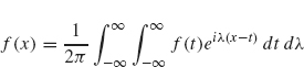
or
We let ![]() (λ) be the quantity inside the parentheses, that is,
(λ) be the quantity inside the parentheses, that is,
![]()
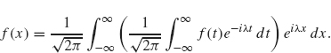
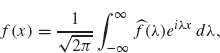
The function ![]() (λ) is called the (complex form of the) Fourier transform of f. Equation (2.2) becomes
(λ) is called the (complex form of the) Fourier transform of f. Equation (2.2) becomes
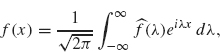
which is often referred to as the Fourier inversion formula, since it describes f(x) as an integral involving the Fourier transform of f.
We summarize this discussion in the following theorem.
Theorem 2.1 If f is a continuously differentiable function with ![]() dt < ∞, then
dt < ∞, then
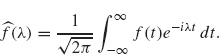
where ![]() (λ) (the Fourier transform of f) is given by
(λ) (the Fourier transform of f) is given by
The preceding argument is not rigorous since we have not justified several steps including the convergence of the improper integral ![]() . As with the development of Fourier series (see Theorem 1.28), if the function f(x) has points of discontinuity, such as a step function, then the preceding formula holds with f(x) replaced by the average of the left- and right-hand limits, that is,
. As with the development of Fourier series (see Theorem 1.28), if the function f(x) has points of discontinuity, such as a step function, then the preceding formula holds with f(x) replaced by the average of the left- and right-hand limits, that is,
Rigorous proofs of these results are given in Appendix A.
The assumption ![]() in Theorem 2.1 assures us that the improper integral defining
in Theorem 2.1 assures us that the improper integral defining ![]() , that is,
, that is,
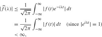
is absolutely convergent. Often, this assumption doesn’t hold. However, in nearly all of the cases in which we are interested, it is not a difficulty if the improper integral is only conditionally convergent. See Example 2.2.
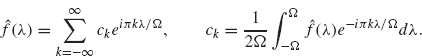
Comparison with Fourier Series. The complex form of the Fourier transform of f and the corresponding inversion formula are analogous to the complex form of the Fourier series of f over the interval –l ≤ x ≤ l:
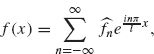
where
The variable λ in the Fourier inversion formula, Eq. (2.3), plays the role of ![]() in Eq. (2.5). The sum over n from –∞ to ∞ in Eq. (2.5) is replaced by an integral with respect to λ from –∞ to ∞ in Eq. (2.3). The formulas for
in Eq. (2.5). The sum over n from –∞ to ∞ in Eq. (2.5) is replaced by an integral with respect to λ from –∞ to ∞ in Eq. (2.3). The formulas for ![]() and
and ![]() (λ) are also analogous. The integral over [–l, l] in the formula for
(λ) are also analogous. The integral over [–l, l] in the formula for ![]() is analogous to the integral over (–∞,∞) in
is analogous to the integral over (–∞,∞) in ![]() (λ). In the case of Fourier series,
(λ). In the case of Fourier series, ![]() measures the component of f which oscillates at frequency n. Likewise,
measures the component of f which oscillates at frequency n. Likewise, ![]() (λ) measures the frequency component of f that oscillates with frequency λ. If f is defined on a finite interval, then its Fourier series is a decomposition of f into a discrete set of oscillating frequencies (i.e.,
(λ) measures the frequency component of f that oscillates with frequency λ. If f is defined on a finite interval, then its Fourier series is a decomposition of f into a discrete set of oscillating frequencies (i.e., ![]() , one for each integer n). For a function on an infinite interval, there is a continuum of frequencies since the frequency component,
, one for each integer n). For a function on an infinite interval, there is a continuum of frequencies since the frequency component, ![]() (λ), is defined for each real number λ. These ideas will be illustrated in the following examples.
(λ), is defined for each real number λ. These ideas will be illustrated in the following examples.
2.1.2 Examples
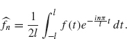
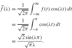
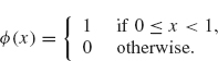
Example 2.2 In our first example, we will compute the Fourier transform of the rectangular wave (see Figure 2.1):
![]()
Figure 2.1. Rectangular wave.
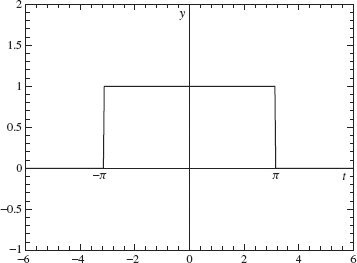
Now, we have ![]() . Since f is an even function, f (t) sin (λt) is an odd function and its integral over the real line is zero. Therefore the Fourier transform of f is reduced to
. Since f is an even function, f (t) sin (λt) is an odd function and its integral over the real line is zero. Therefore the Fourier transform of f is reduced to
A graph of ![]() is given in Figure 2.2.
is given in Figure 2.2.
As already mentioned, the Fourier transform, ![]() (λ), measures the frequency component of f that vibrates with frequency λ. In this example, f is a piece wise constant function. Since a constant vibrates with zero frequency, we should expect that the largest values of
(λ), measures the frequency component of f that vibrates with frequency λ. In this example, f is a piece wise constant function. Since a constant vibrates with zero frequency, we should expect that the largest values of ![]() (λ) occur when λ is near zero. The graph of
(λ) occur when λ is near zero. The graph of ![]() in Figure 2.2 clearly illustrates this feature.
in Figure 2.2 clearly illustrates this feature.
This example also illustrates the inversion formula when there is a jump discontinuity. By Eq. (2.4), we have that
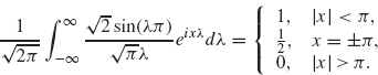
Figure 2.2. Fourier transform of a rectangular wave.
The improper integral above is conditionally convergent, rather than absolutely convergent, because ![]() . Even so, the inversion formula is still valid.
. Even so, the inversion formula is still valid.
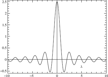
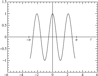
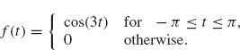
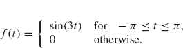
Example 2.3 Let
![]()
(see Figure 2.3).
Since f is an even function, only the cosine part of the transform contributes:
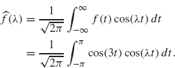
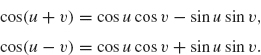
The preceding integral is left as an exercise (sum the two identities
![]()
with u = 3t and v = λt and then integrate). The result is
![]()
Figure 2.3. Plot of cos(3f).
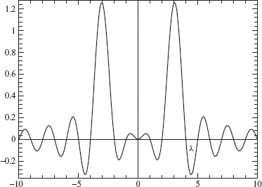
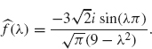
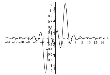
The graph of ![]() is given in Figure 2.4.
is given in Figure 2.4.
Note that the Fourier transform peaks at λ = 3 and –3. This should be expected since f(t) = cos(3t) vibrates with frequency 3 on the interval –π ≤ t ≤ t ≤ π.
Figure 2.4. Fourier transform of cos(3f).
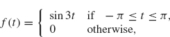
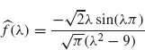
Example 2.4 Let
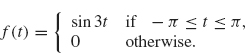
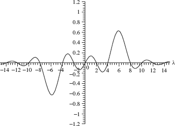
Since f is an odd function, only the sine part of the transform contributes (which is purely imaginary). The transform is
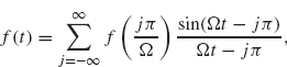
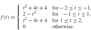
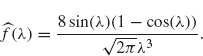
Example 2.5 The next example is a triangular wave whose graph is given in Figure 2.5. An analytical formula for this graph is given by
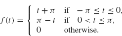
Figure 2.5. Triangular wave.
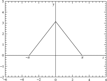
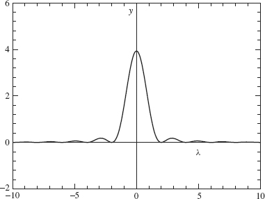
This function is even and so its Fourier transform is given by
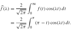
This integral can be computed using integration by parts:
![]()
The graph of ![]() is given in Figure 2.6.
is given in Figure 2.6.
Note that the Fourier transforms in Examples 2.4 and 2.5 decay at the rate l/λ2 as λ ![]() ∞ which is faster than the decay rate of 1/λ. exhibited by the Fourier transforms in Examples 2.2 and 2.3. The faster decay in Examples 2.4 and 2.5 results from the continuity of the functions in these examples. Note the parallel with the examples in Chapter 2. The Fourier coefficients, an and bn, for the discontinuous function in Example 1.9 decay like l/n, whereas the Fourier coefficients for the continuous function in Example 1.10 decay like 1/n2.
∞ which is faster than the decay rate of 1/λ. exhibited by the Fourier transforms in Examples 2.2 and 2.3. The faster decay in Examples 2.4 and 2.5 results from the continuity of the functions in these examples. Note the parallel with the examples in Chapter 2. The Fourier coefficients, an and bn, for the discontinuous function in Example 1.9 decay like l/n, whereas the Fourier coefficients for the continuous function in Example 1.10 decay like 1/n2.
Figure 2.6. Fourier transform of the triangular wave.
2.2 PROPERTIES OF THE FOURIER TRANSFORM
2.2.1 Basic Properties
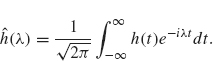
In this section we set down most of the basic properties of the Fourier transform. First, we introduce the alternative notation
![]()
for the Fourier transform of f. This notation has advantages when discussing some of the operator theoretic properties of the Fourier transform. The Fourier operator ![]() should be thought of as a mapping whose domain and range is the space of complex-valued functions defined on the real line. The input of T is a function, say f, and returns another function,
should be thought of as a mapping whose domain and range is the space of complex-valued functions defined on the real line. The input of T is a function, say f, and returns another function, ![]() [f] =
[f] = ![]() , as its output.
, as its output.
In a similar fashion, we define the inverse Fourier transform operator as
![]()
Theorem 2.1 implies that ![]() –1 really is the inverse of
–1 really is the inverse of ![]()
because
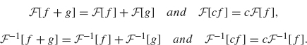
Some properties of the Fourier transform and its inverse are given in the following theorem. Other basic properties will be given in the exercises.
Theorem 2.6 Let f and g be differentiable functions defined on the real line with f (t) = 0 for large |t|. The following properties hold.
1. The Fourier transform and its inverse are linear operators. That is, for any constant c we have
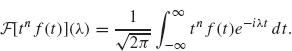
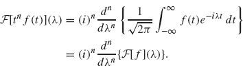
2. The Fourier transform of a product of f with tn is given by
![]()
3. The inverse Fourier transform of a product of f with λn is given by
![]()
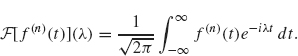
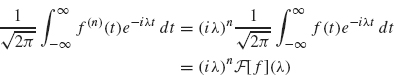
4. The Fourier transform of an nth derivative is given by
![]()
(here, f(n) stands for the nth derivative of f.
5. The inverse Fourier transform of an nth derivative is given by
![]()
6. The Fourier transform of a translation is given by
![]()
7. The Fourier transform of a rescaling is given by
![]()
8. If f (t) = 0 for t < 0, then
![]()
where ![]() [f] is the Laplace transform of f defined by
[f] is the Laplace transform of f defined by
![]()
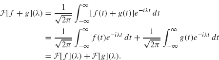
Proof. We prove each part separately.
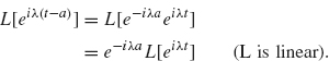
1. The linearity of the Fourier transform follows from the linearity of the integral as we demonstrate in the following:
The proof for ![]() [cf] = c
[cf] = c![]() [f] is similar as are the proofs for the corresponding facts for the inverse Fourier transform.
[f] is similar as are the proofs for the corresponding facts for the inverse Fourier transform.
2 and 3. For the Fourier transform of a product of f with tn, we have
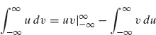
Using
![]()
we obtain
The corresponding property for the inverse Fourier transform is proved similarly.
4 and 5. For the Fourier transform of the nth derivative of f, we have
Now, we integrate by parts:
with dv = f(n) and u = e–iλt. As we will see, this process has the effect of transferring the derivatives from f(n) to e–λt. Since f vanishes at +∞ and –∞ by hypothesis, there are no boundary terms. So we have
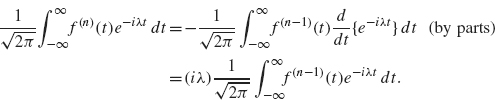
Note that integration by parts has reduced the number of derivatives on f by one (f(n) becomes f(n–1)). We have also gained one factor of ik. By repeating this process n – 1 additional times, we obtain
as desired. The proof for the corresponding fact for the inverse Fourier transform is similar.
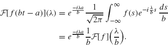
6 and 7. The translation and rescaling properties can be combined into the following statement:
This equation can be established by the following change of variables argument:
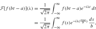
where the second equality follows from the change of variables s = bt – a (and so t = (s + a)/b and dt = ![]() ). Rewriting the exponential on the right as
). Rewriting the exponential on the right as
![]()
we obtain
8. The final part of the theorem, regarding the relationship of the Fourier and Laplace transforms, follows from their definitions and is left to the exercises. This completes the proof. I
Example 2.7 We illustrate the fourth property of Theorem 2.6 with the function in Example 2.4:
whose Fourier transform is
The derivative of f is 3 cos 3t on –π ≤ t ≤ π, which is just a multiple of 3 times the function given in Example 2.3. Therefore from Example 2.3 we have
The fourth property of Theorem 2.6 (with n = 1) states
![]()
This expression for ![]() ′(λ) agrees with Eq. (2.8).
′(λ) agrees with Eq. (2.8).
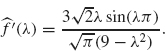
Example 2.8 In this example, we illustrate the scaling property:
If b > 1, then the graph of f (bt) is a compressed version of the graph of f. The dominant frequencies of f (bt) are larger than those of f by a factor of b. This behavior is illustrated nicely by the function in Example 2.4:
![]()
whose graph is given in Figure 2.7. The graph of f(2t) is given in Figure 2.8. Note the frequency f (2t) is double that off.
Increasing the frequency of a signal has the effect of stretching the graph of its Fourier transform. In the preceding example, the dominant frequency of f (t) is 3, whereas the dominant frequency of f (2t) is 6. Thus the maximum value of |![]() (λ)| occurs at λ = 3 (see Figure 2.9) whereas the maximum value of the
(λ)| occurs at λ = 3 (see Figure 2.9) whereas the maximum value of the
Figure 2.7. Plot of sin(3t) –π ≤ t ≤ π.
Figure 2.8. Plot of sin(6t) –π/2 ≤ t ≤ π/2.
Figure 2.9. Plot of Fourier transform of sin(3f ).
Fourier transform of f (2t) occurs at λ = 6 (see Figure 2.10). Thus the latter graph is obtained by stretching the former graph by a factor of 2. Note also that the graph of ![]() (λ/2) is obtained by stretching the graph of
(λ/2) is obtained by stretching the graph of ![]() (λ) by a factor of 2.
(λ) by a factor of 2.
This discussion illustrates the following geometrical interpretation of Eq. (2.9) in the case where b > 1: Compressing the graph of f speeds up the frequency
Figure 2.10. Plot of Fourier transform of sin(6f).
and therefore stretches the graph of ![]() (λ). If 0 < b < 1, then the graph of f(bt) is stretched, which slows the frequency and therefore compresses the graph of
(λ). If 0 < b < 1, then the graph of f(bt) is stretched, which slows the frequency and therefore compresses the graph of ![]() (λ)
(λ)
2.2.2 Fourier Transform of a Convolution
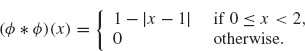
Now we examine how the Fourier transform behaves under a convolution, which is one of the basic operations used in signal analysis. First, we give the definition of the convolution of two functions.
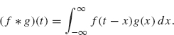
Definition 2.9 Suppose f and g are two square-integrable functions. The convolution of f and g, denoted f * g, is defined by
The preceding definition is equivalent to
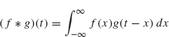
(perform the change of variables y = t – x and then relabel the variable y back to x).
We have the following theorem on the Fourier transform of a convolution of two functions.
Theorem 2.10 Suppose f and g are two integrable functions. Then
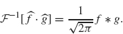
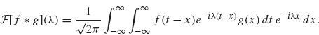
Proof. To derive the first equation, we use the definitions of the Fourier transform and convolution:
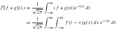
We write ![]() . After switching the order of integration, we obtain
. After switching the order of integration, we obtain
Letting s = t – x, we obtain
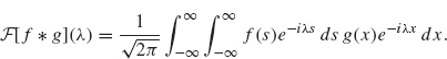
The right side can be rewritten as
![]()
which is ![]() , as desired.
, as desired.
Equation (2.11) follows from Eq. (2.10) and the inverse formula for the Fourier transform as follows:
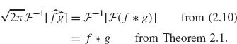
This completes the proof of the theorem.
2.2.3 Adjoint of the Fourier Transform
Recall that the adjoint of a linear operator T : V ![]() W between inner product spaces is an operator T* : W
W between inner product spaces is an operator T* : W ![]() V such that
V such that
![]()
In the next theorem, we show that the adjoint of the Fourier transform is the inverse of the Fourier transform.
Theorem 2.11 Suppose f and g are square integrable. Then
![]()
Proof. We have:
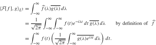
(by switching the order of integration). The second integral (involving g) is ![]() therefore
therefore
as desired.
2.2.4 Plancherel Theorem
The Plancherel formula states that the Fourier transform preserves the L2 inner product.
Theorem 2.12 Suppose f and g are square integrable. Then
In particular,
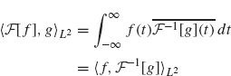
Proof. Equation (2.12) follows from Theorems 2.11 and 2.1 as follows:
as desired. Equation (2.13) can be established in a similar manner. Equation (2.14) follows from (2.12) with f = g.
Remark. The equation ![]() is analogous to Eq. (1.41), and is also referred to as Parseval’s equation. It has the following interpretations. For a function, f, defined on [–π, π], let
is analogous to Eq. (1.41), and is also referred to as Parseval’s equation. It has the following interpretations. For a function, f, defined on [–π, π], let ![]() (f)(n) be its nth Fourier coefficient (except with the factor
(f)(n) be its nth Fourier coefficient (except with the factor ![]() instead of 1/2π):
instead of 1/2π):
![]()
Equation (1.41) can be restated as
![]()
which is analogous to (2.14) for the Fourier transform with l2 and L2[–π, π] replaced by the L2 norm on the entire real line. As in the case with Fourier series, Plancherel’s Theorem states that the energy of a signal in the time domain, ![]() , is the same as the energy in the frequency domain
, is the same as the energy in the frequency domain ![]()
2.3.1 Time-Invariant Filters
The Fourier transform plays a central role in the design of filters. A filter can be thought of as a “black box” that takes an input signal, processes it, and then returns an output signal that in some way modifies the input. One example of a filter is a device that removes noise from a signal.
From a mathematical point of view, a signal is a function f : R ![]() C that is piecewise continuous. A filter is a transformation L that maps a signal,f, into another signal
C that is piecewise continuous. A filter is a transformation L that maps a signal,f, into another signal ![]() . This transformation must satisfy the following two properties in order to be a linear filter:
. This transformation must satisfy the following two properties in order to be a linear filter:
- Additivity: L[f + g] = L[f] + L[g]
- Homogeneity: L[cf] = cL[f], where c is a constant.
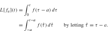
There is another property that we want our filter L to have. If we play an old, scratchy record for half an hour starting at 3 pm today and put the signal through a noise reducing filter, we want to hear the cleaned-up output, at roughly the same time as we play the record. If we play the same record at 10 am tomorrow morning and use the same filter, we should hear the identical output, again at roughly the same time. This property is called time invariance. To formulate this concept, we introduce the following notation: For a function f(t) and a real number a, let fa(t) = f(t – a). Thus fa is a time shift, by a units, of the signal f.
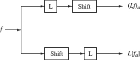
Definition 2.13 A transformation L (mapping signals to signals) is said to be time-invariant if for any signal f and any real number a, L[fa](t) = (Lf)(t – a) for all t (or L[fa] = (Lf)a). In words, L is time-invariant if the time-shifted input signal f(t – a) is transformed by L into the time-shifted output signal (Lf)(t – a). (See Figure 2.11.)
Example 2.14 Let l(t) be a function that has finite support (i.e., l(t) is zero outside of a finite t-interval). For a signal f, let
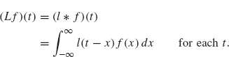
This linear operator is time-invariant because for any a ∈ R
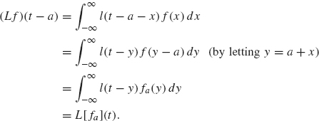
Thus, (Lf)(t – a) = L[fa)](t) and so L is time-invariant.
Not every linear transformation has this property, as the following example shows.
Figure 2.11. L is time-invariant if the upper and lower outputs are the same.
Example 2.15 Let
On one hand, we have
On the other hand, we obtain
![]()
Since L[fa](t) and (Lf)(t – a) are not the same (for a ≠ 0), L is not time-invariant. ¦
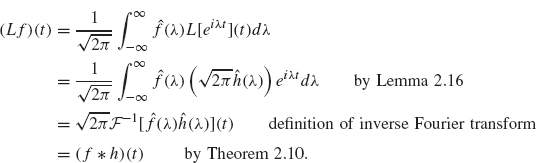
The next lemma and theorem show that the convolution in Example 2.14 is typical of time-invariant linear niters. We start by computing L(eiλt).
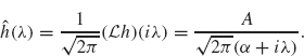
Lemma 2.16 Let L be a linear, time-invariant transformation and let λ be any fixed real number. Then, there is a function h with
![]()
Remark. Note that the input signal eiλt is a (complex-valued) sinusoidal signal with frequency λ. This lemma states that the output signal from a time-invariant filter of a sinusoidal input signal is also sinusoidal with the same frequency.
Proof. Our proof is somewhat informal in order to clearly explain the essential ideas. Let hλ(t) = L(eiλt). Since L is time-invariant, we have
for each real number a. Since L is linear, we also have
Thus
Comparing Eqs. (2.15) and (2.16), we find
![]()
Since a is arbitrary, we may set a = t yielding hλ(0) = e–iλthλ(t); solving for hx(t), we obtain
![]()
Letting ![]() (λ) = hλ(0)/
(λ) = hλ(0)/![]() completes the proof.
completes the proof.
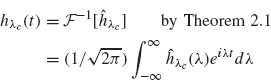
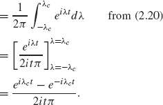
The function ![]() (λ) determines L. To see this, we first use the Fourier Inversion Theorem (Theorem 2.1)
(λ) determines L. To see this, we first use the Fourier Inversion Theorem (Theorem 2.1)
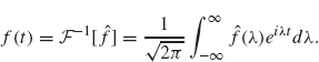
Then we apply L to both sides:
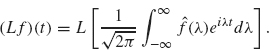
The integral on the right can be approximated by a Riemann sum:
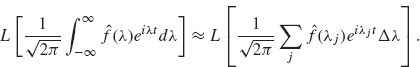
Since L is linear, we can distribute L across the sum:
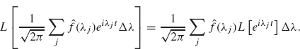
As the partition gets finer, the Riemann sum on the right becomes an integral and so from (2.17), (2.18), and (2.19), we obtain
Even though the preceding argument is not totally rigorous, the result is true with very few restrictions on either L or the space of signals being considered (see the text on Fourier analysis by Stein and Weiss (1971) for more details). We summarize this discussion in the following theorem.
Theorem 2.17 Let L be a linear, time-invariant transformation on the space of signals that are piecewise continuous functions. Then there exists an integrable function, h, such that
![]()
for all signalsf.
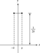
Physical Interpretation. Both h(t) and ![]() (λ) have physical interpretations. Assume that h(t) is continuous and that δ is a small positive number. We apply L to the impulse signal
(λ) have physical interpretations. Assume that h(t) is continuous and that δ is a small positive number. We apply L to the impulse signal
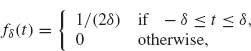
whose graph is given in Figure 2.12. Note that ![]() . Applying L to fδ, we obtain
. Applying L to fδ, we obtain
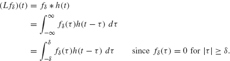
Figure 2.12. Graph of fδ.
Since h is continuous, h(t – τ) is approximately equal to h(t) for |τ| ≤ δ. Therefore
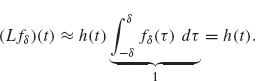
Thus h(t) is the approximate response to an input signal which is an impulse. For that reason, h(t) is called the impulse response function.
We have already seen that ![]() . Thus up to a constant factor,
. Thus up to a constant factor, ![]() (λ) is the amplitude of the response to a “pure frequency” signal eiλt; is called the system function.
(λ) is the amplitude of the response to a “pure frequency” signal eiλt; is called the system function.
2.3.2 Causality and the Design of Filters
Designing a time-invariant filter is equivalent to constructing the impulse function, h, since any such filter can be written as
![]()
by Theorem 2.17. The construction of h depends on what the filter is designed to do. In this section, we consider filters that reduce high frequencies, but leave the low frequencies virtually unchanged. Such filters are called low-pass filters.
Taking the Fourier transform of both sides of Lf = f * h and using Theorem 2.10 yields
![]()
A Faulty Filter. Suppose we wish to remove all frequency components from the signal f that lie beyond some cutoff frequency λc. As a natural first attempt, we choose an h whose Fourier transform is zero outside of the interval –λc ≤ λ ≤ λc:
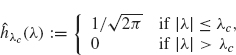
(the choice of constant ![]() is for convenience in later calculations). Since
is for convenience in later calculations). Since ![]() is zero for |λ| > λc, this filter at least appears to remove the unwanted frequencies (above λc) from the signal f. However, we will see that this filter is flawed in other respects.
is zero for |λ| > λc, this filter at least appears to remove the unwanted frequencies (above λc) from the signal f. However, we will see that this filter is flawed in other respects.
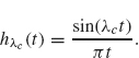
The impulse response function corresponding to the system function hXc is easy to calculate:
Therefore
Now we filter the following simple input function:
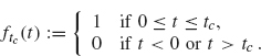
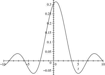
Think of ftc as a signal that is “on” for t between 0 and tc and off at other times. The effect of this filter on the signal ftc is
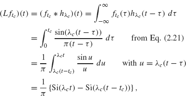
where ![]() . A plot of
. A plot of ![]() with tc and λc both 1 is given in Figure 2.13. Note that the graph of the output signal is nonzero for t < 0, whereas the input signal, ftc(t), is zero for t < 0. This indicates that the output signal occurs before the input signal has arrived! Clearly, a filter cannot be physically constructed to produce an output signal before receiving an input signal. Thus, our first attempt at constructing a filter by using the function hλc is not practical. The following definition and theorem characterize a more realistic class of filters.
with tc and λc both 1 is given in Figure 2.13. Note that the graph of the output signal is nonzero for t < 0, whereas the input signal, ftc(t), is zero for t < 0. This indicates that the output signal occurs before the input signal has arrived! Clearly, a filter cannot be physically constructed to produce an output signal before receiving an input signal. Thus, our first attempt at constructing a filter by using the function hλc is not practical. The following definition and theorem characterize a more realistic class of filters.
Causal Filters
Definition 2.18 A causal filter is one for which the output signal begins after the input signal has started to arrive.
The following result tells us which filters are causal.
Figure 2.13. Graph of ± {Si(f) – Si(f – 1)}.
Theorem 2.19 Let L be a time-invariant filter with response function h (i.e., Lf = f * h). L is a causal filter if and only if h(t) = 0 for all t < 0.
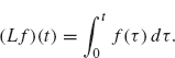
Proof. We prove that if h(t) = 0 for all t < 0, then the corresponding filter is causal. We leave the converse as an exercise (see exercise 8). We first show that if f (t) = 0 for t < 0, then (Lf)(t) = 0 for t < 0. We have
![]()
where the lower limit in the integral is 0 because f (τ) = 0 when τ < 0. If t < 0 and τ ≥ 0, then t – τ < 0 and so h(t – τ) = 0, by hypothesis. Therefore, (Lf)(t) = 0 for t < 0. We have therefore shown that if f (t) = 0 for t < 0, then (Lf)(t) = 0 for t < 0. In other words, if the input signal does not arrive until t = 0, the output of the filter also does not begin until t = 0.
Suppose more generally that the input signal f does not arrive until t = a. To show that L is causal, we must show that Lf does not begin until t = a. Let g(t) = f (t + a). Note that the signal g(t) begins at t = 0. From the previous paragraph, (Lg)(t) does not begin until t = 0. Since f (t) = g(t – a) = ga(t), we have
Since (Lg)(τ) does not begin until τ = 0, we see that (Lg)(t – a) does not begin until t = a. Thus (Lf)(t) = (Lg)(t – a) does not begin until t = a, as desired.
Theorem 2.19 applies to the response function, but it also gives us important information about ![]() (λ). By the definition of the Fourier transform:
(λ). By the definition of the Fourier transform:
If the filter associated to h is causal, Theorem 2.19 implies h(t) = 0 for t < 0 and so
We summarize this discussion in the following theorem.
Theorem 2.20 Suppose L is a causal filter with response function h. Then the system function associated with L is
where ![]() is the Laplace transform.
is the Laplace transform.
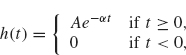
Example 2.21 One of the older causal, noise-reducing filters is the Butterworth filter (Papoulis, 1962). It is constructed using the previous theorem with
![]()
where A and a are positive parameters. Its Fourier transform is given by
(see Exercise 10). Note that ![]() (λ) decays as λ
(λ) decays as λ ![]() ∞, thus diminishing the high frequency components of the filtered signal
∞, thus diminishing the high frequency components of the filtered signal ![]() .
.
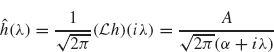
Consider the signal given by
![]()
whose graph is given in Figure 2.14. We wish to filter the noise that vibrates with frequency approximately 40. At the same time, we do not want to disturb the basic shape of this signal, which vibrates in the frequency range of 2–4 By choosing A = α = 10, ![]() (λ) is close to
(λ) is close to ![]() (0) =
(0) = ![]() for |λ| ≤ 4; but
for |λ| ≤ 4; but ![]() (λ)| is small (less than 0.1) when λ ≥ 40. Thus filtering by h with this choice of parameters A and α should preserve the low frequencies (frequency ≤ 4) while damping the high frequencies (> 40). A plot of the filtered signal (f * h)(t) for 0 ≤ t ≤ π is given in Figure 2.15. Most of the high-frequency noise has been filtered. Most of the low-frequency components of this signal have been preserved.
(λ)| is small (less than 0.1) when λ ≥ 40. Thus filtering by h with this choice of parameters A and α should preserve the low frequencies (frequency ≤ 4) while damping the high frequencies (> 40). A plot of the filtered signal (f * h)(t) for 0 ≤ t ≤ π is given in Figure 2.15. Most of the high-frequency noise has been filtered. Most of the low-frequency components of this signal have been preserved.
Figure 2.14. Graph of e–t/3 (sin 2t + 2sin4t + 0.4sin2t sin40t).
Figure 2.15. Graph of the filtered signal from Figure 2.14.
In this section we examine a class of signals (i.e., functions) whose Fourier transform is zero outside a finite interval [–Ω, Ω]; these are (frequency) band-limited functions. For instance, the human ear can only hear sounds with frequencies less than 20 kHz (1 kHz = 1000 cycles per second). Thus, even though we make sounds with higher pitches, anything above 20 kHz can’t be heard. Telephone conversations are thus effectively band-limited signals. We will show below that a band-limited signal can be reconstructed from its values (or samples) at regularly spaced times. This result is basic in continuous-to-digital signal processing.
Definition 2.22 A function f is said to be frequency band-limited if there exists a constant Ω > 0 such that
![]()
When Q is the smallest frequency for which the preceding equation is true, the natural frequency v := ![]() is called the Nyquist frequency, and 2v =
is called the Nyquist frequency, and 2v = ![]() is the Nyquist rate.
is the Nyquist rate.
Theorem 2.23 (Shannon-Whittaker Sampling Theorem). Suppose that ![]() (λ) is piecewise smooth and continuous and that
(λ) is piecewise smooth and continuous and that ![]() , where Ω is some fixed, positive frequency. Then f =
, where Ω is some fixed, positive frequency. Then f = ![]() –1[
–1[![]() ] is completely determined by its values at the points tj = jπ/Ω, j = 0, ±1, ±2, .... More precisely, f has the following series expansion:
] is completely determined by its values at the points tj = jπ/Ω, j = 0, ±1, ±2, .... More precisely, f has the following series expansion:
where the series on the right converges uniformly.
This is a remarkable theorem! Let’s look at how we might use it to transmit several phone conversations simultaneously on a single wire (or channel). As mentioned earlier, phone conversations are band-limited. In fact the dominant frequencies are below 1 kHz, which we will take as our Nyquist frequency. The Nyquist rate v = ![]() is then double this, or 2 kHz; so we need to sample the signal every
is then double this, or 2 kHz; so we need to sample the signal every ![]() millisecond. How many phone conversations can we send in this manner? Transmission lines typically send about 56 thousand bits per second. If each sample can be represented by 7 bits, then we can transmit 8 thousand samples per second, or 8 every millisecond, or 4 every half millisecond. By tagging and interlacing signals, we can transmit the samples from four conversations. At the receiver end, we can use the series in Eq. (2.22) to reconstruct the signal, with the samples being f(
millisecond. How many phone conversations can we send in this manner? Transmission lines typically send about 56 thousand bits per second. If each sample can be represented by 7 bits, then we can transmit 8 thousand samples per second, or 8 every millisecond, or 4 every half millisecond. By tagging and interlacing signals, we can transmit the samples from four conversations. At the receiver end, we can use the series in Eq. (2.22) to reconstruct the signal, with the samples being f(![]() j) for j an integer and time in milliseconds (only a finite number of these occur during the life of a phone conversation–unless perhaps a teenager is on the line). Here is the proof of the theorem.
j) for j an integer and time in milliseconds (only a finite number of these occur during the life of a phone conversation–unless perhaps a teenager is on the line). Here is the proof of the theorem.
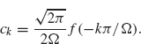
Proof. Using Theorem 1.20 (with a = Ω and t = λ), we expand ![]() (λ) in a Fourier series on the interval [–Ω, Ω]:
(λ) in a Fourier series on the interval [–Ω, Ω]:
Since ![]() (λ) = 0 for |λ| ≥ Ω, the limits in the integrals defining ck can be changed to –∞ and ∞:
(λ) = 0 for |λ| ≥ Ω, the limits in the integrals defining ck can be changed to –∞ and ∞:
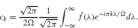
By Theorem 2.1,
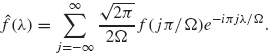
If we use this expression for ck in the preceding series, and if at the same time we change the summation index from k to j = –k, we obtain
Since ![]() is a continuous, piecewise smooth function, the series (2.23) converges uniformly by Theorem 1.30. Using Theorem 2.1, we obtain
is a continuous, piecewise smooth function, the series (2.23) converges uniformly by Theorem 1.30. Using Theorem 2.1, we obtain
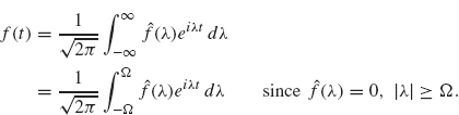
Using Eq. (2.23) for ![]() and interchanging the order of integration and summation, we obtain
and interchanging the order of integration and summation, we obtain
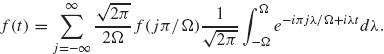
The integral in Eq. (2.24) is
![]()
After simplifying Eq. (2.24), we obtain Eq. (2.22), which completes the proof.
The convergence rate in Eq. (2.22) is rather slow since the coefficients (in absolute value) decay like 1/j. The convergence rate can be increased so that the terms behave like 1/j2 or better, by a technique called over sampling, which is discussed in exercise 14. At the opposite extreme, if a signal is sampled below the Nyquist rate, then the signal reconstructed via Eq. (2.22) will not only be missing high-frequency components, but will also have the energy in those components transferred to low frequencies that may not have been in the signal at all. This is a phenomenon called aliasing.
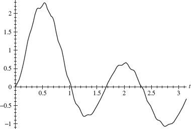
Example 2.24 Consider the function f defined by
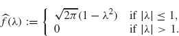
We can calculate f(t) = T x[/] by computing
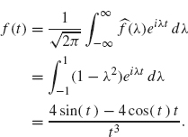
The last equality can be obtained by integration by parts (or by using your favorite computer algebra system). The plot of f is given in Figure 2.16.
Figure 2.16. Graph off.
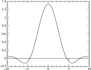
Figure 2.17. Graph of partial series in Sampling Theorem with í2 = 1.
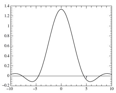
Since ![]() (λ) = 0 for |λ| > 1, the frequency Ω from the Sampling Theorem can be chosen to be any number that is greater than or equal to 1 With Ω = 1, we graph the partial sum of the first 30 terms in the series given in the Sampling Theorem in Figure 2.17; note that the two graphs are nearly identical.
(λ) = 0 for |λ| > 1, the frequency Ω from the Sampling Theorem can be chosen to be any number that is greater than or equal to 1 With Ω = 1, we graph the partial sum of the first 30 terms in the series given in the Sampling Theorem in Figure 2.17; note that the two graphs are nearly identical.
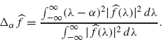
In this section we present the Uncertainty Principle, which in words states that a function cannot simultaneously have restricted support in time as well as in frequency. To explain these ideas, we need a definition.
Definition 2.25 Suppose f is a function in L2(R). The dispersion of f about the point a ∈ R is the quantity
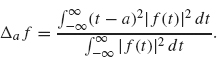
The dispersion of f about a point a measures the deviation or spread of its graph from t = a. This dispersion will be small if the graph of f is concentrated near t = a, as in Figure 2.18 (with a = 0). The dispersion will be larger if the graph of f spreads out away from t = a as in Figure 2.19.
Another description of the dispersion is related to statistics. Think of the function ![]() as a probability density function (this nonnegative function has integral equal to one, which is the primary requirement for a probability density function). If a is the mean of this density, then Δa f is just the variance.
as a probability density function (this nonnegative function has integral equal to one, which is the primary requirement for a probability density function). If a is the mean of this density, then Δa f is just the variance.
Figure 2.18. Small dispersion off5.
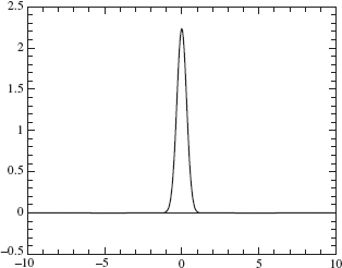
Figure 2.19. Larger dispersion of f1.
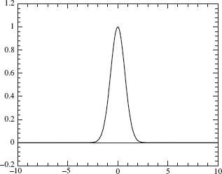
Applying the preceding definition of dispersion to the Fourier transform off gives
By the Plancherai Theorem (Theorem 2.12), the denominators in the dispersions of f and ![]() are the same.
are the same.
If the dispersion of ![]() about λ = α is small, then the frequency range of f is concentrated near λ = α.
about λ = α is small, then the frequency range of f is concentrated near λ = α.
Now we are ready to state the Uncertainty Principle.
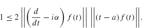
Theorem 2.26 (Uncertainty Principle). Suppose f is a function in L2(R) which vanishes at +∞ and –∞. Then
for all points a ∈ R and α ∈ R.
One consequence of the Uncertainty Principle is that the dispersion of f about any a (i.e., Δa f) and the dispersion of the Fourier transform of f about any frequency α (i.e., Δα![]() ) cannot simultaneously be small. The graph in Figure 2.18 offers an intuitive explanation. This graph is concentrated near t = 0, and therefore its dispersion about t = 0 is small. However, this function changes rapidly, and therefore it will havejarge-frequency components in its Fourier transform. Thus, the dispersion of
) cannot simultaneously be small. The graph in Figure 2.18 offers an intuitive explanation. This graph is concentrated near t = 0, and therefore its dispersion about t = 0 is small. However, this function changes rapidly, and therefore it will havejarge-frequency components in its Fourier transform. Thus, the dispersion of ![]() about any frequency value will be large. This is illustrated by the wide spread of the graph of its Fourier transform, given in Figure 2.20.
about any frequency value will be large. This is illustrated by the wide spread of the graph of its Fourier transform, given in Figure 2.20.
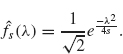
For a more quantitative viewpoint, suppose
![]()
Figure 2.20. Large-frequency dispersion of ![]() 5
5
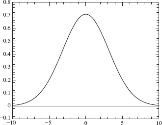
The graphs of fs for s = 5 and s = 1 are given in Figures 2.18 and 2.19, respectively. Note that as s increases, the exponent becomes more negative and therefore the dispersion of fs decreases (i.e., the graph of fs becomes more concentrated near the origin).
The Fourier transform of fs is
![]()
(see exercise 6). Except for the constant in front, the Fourier transform of fs has the same general negative exponential form as does fs. Thus the graph of ![]() s has the same general shape as does the graph of fs. There is one notable difference: The factor s appears in the denominator of the exponent in
s has the same general shape as does the graph of fs. There is one notable difference: The factor s appears in the denominator of the exponent in ![]() s instead of the numerator ofthe exponent (as is the case for fs). Therefore, as s increases, the dispersion of
s instead of the numerator ofthe exponent (as is the case for fs). Therefore, as s increases, the dispersion of ![]() s also increases (instead of decreasing as it does for fs). In particular, it is not possible to choose a value of s that makes the dispersions of both fs and
s also increases (instead of decreasing as it does for fs). In particular, it is not possible to choose a value of s that makes the dispersions of both fs and ![]() s simultaneously small.
s simultaneously small.
Proof of Uncertainty Principle. We first claim that the following identity holds:
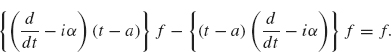
Here, α and a are real constants. Written out in detail, the left side is
![]()
After using the product rule for the first term and then simplifying, the result isf, which establishes Eq. (2.26).
Note that Eq. (2.26) remains valid after dividing both sides by the constant ||f|| = ||f||L2. Since the L2 norm of f/||f|| is one, we may as well assume from the start that ||f|| = 1 (just by relabeling f/||f|| as f.
Now take the L2 inner product of both sides of Eq. (2.26). The result is
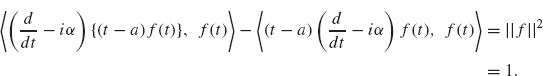
Both terms on the left involve integrals (from –∞ to ∞). We use integration by parts on the first integral on the left and use the assumption that f (–∞) = f (∞) = 0. The result is
(the details of which we ask you to carry out in exercise 9).
From Eq. (2.28) and the triangle inequality, we obtain
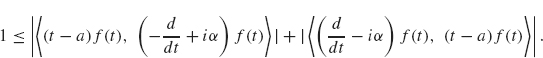
Now apply Schwarz’s inequality (see Theorem 0.11) to the preceding two inner products:
Next, we apply the Plancherel formula (Theorem 2.12) and the fourth property of Theorem 2.6 to obtain
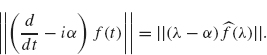
Combining this equation with the previous inequality, we get
![]()
Since ||f ||L2 = 1 = || ||L2, we have
![]()
Therefore, squaring both sides of the preceding inequality yields
![]()
which completes the proof of the Uncertainty Principle. (Note: This proof is based on that given for the quantum mechanical version by H. P. Robertson, Phys. Rev. 34, 163-164 (1929)).
1. Let
Show that
![]()
where m is an integer and λ ≠ m. Hint: Sum the two identities
Use this integral to show
as indicated in Example 2.3.
2. Let
Compute ![]() (λ) (i.e., provide the details for Example 2.4).
(λ) (i.e., provide the details for Example 2.4).
3. (Note: A computer algebra system would help for this problem). Let
Show that f and f′ are continuous everywhere (pay particular attention to what happens at t = –2, – 1, L and 2). Draw a careful graph off. Compute its Fourier transform and show that
Plot the Fourier transform over the interval –10 ≤ λ ≤ 10. Note that the Fourier transform decays like ![]() as λ
as λ ![]() ∞. Note that in exercise 1 the given function is discontinuous and
∞. Note that in exercise 1 the given function is discontinuous and ![]() (λ) decays like
(λ) decays like ![]() as λ
as λ ![]() ∞; in exercise 2, f is continuous, but not differentiable and
∞; in exercise 2, f is continuous, but not differentiable and ![]() (λ) decays like 1/λ2. Do you see a pattern?
(λ) decays like 1/λ2. Do you see a pattern?
4.Suppose f ∈ L2(–∞, ∞) is a real-valued, even function; show that ![]() is real-valued. Suppose f ∈ L2(–∞, ∞) is a real-valued, odd function; show that
is real-valued. Suppose f ∈ L2(–∞, ∞) is a real-valued, odd function; show that ![]() (λ) is pure imaginary (its real part is zero) for each λ.
(λ) is pure imaginary (its real part is zero) for each λ.
5.Let
Show that
6. Let fs(x) = √se–sx2. Show that
Hint: After writing out the definition of the Fourier transform, complete the square in the exponent, then perform a change of variables in the resulting integral (a complex translation) and then use the fact that ![]() .
.
7.Establish the parts of Theorem 2.6 that deal with the inverse Fourier transform. Establish the relationship between the Fourier transform and the Laplace transform given in the last part of this theorem.
8.Suppose L is a time invariant filter with a continuous response function h (see Theorem 2.19). Show that if L is causal then h(t) =0 for t < 0. Hint: Prove by contradiction—Assume h(t0) ≠ 0 for some t0 < 0; show that by choosing an appropriate f which is nonzero only on the interval [0, δ] for some very small δ > 0, that L(f)(t) > 0 for some t < 0 even though f(t) = 0 for all t < 0 (thus contradicting causality).
9. Using integration by parts, show that Eq. (2.28) follows from Eq. (2.27).
10. Let
where A and a are parameters as in Example 2.21. Show that
11. Consider the signal
![]()
Filter this signal with the Butterworth filter (i.e., compute (f * h)(t)) for 0 ≤ t ≤ π. Try various values of A = α (starting with A = α = 10). Compare the filtered signal with the original signal.
12. Consider the filter given by f ![]() f * h, where
f * h, where
Compute and graph ![]() (λ) for 0 ≤ λ ≤ 20. for various values of d. Suppose you wish to use this filter to remove signal noise with frequency larger than 30 and retain frequencies in the range of 0 to 5 (cycles per 2π interval). What values of d would you use? Filter the signal
(λ) for 0 ≤ λ ≤ 20. for various values of d. Suppose you wish to use this filter to remove signal noise with frequency larger than 30 and retain frequencies in the range of 0 to 5 (cycles per 2π interval). What values of d would you use? Filter the signal
![]()
with your chosen values of d and compare the graph of the filtered signal with the graph off.
13. The Sampling Theorem (Theorem 2.23) states that if the Fourier transform of a signal f is band-limited to the interval [–Ω, Ω], then the signal can be recovered by sampling the signal at a grid of time nodes separated by a time interval of π/Ω. Now suppose that the Fourier transform of a signal, f, vanishes outside the interval [ω1 ≤ λ ≤ ω2]; develop a formula analogous to Eq. (2.22) where the time interval of separation is 2π/(ω2 – ω1). Hint: Show that the Fourier transform of the signal
![]()
is band-limited to the interval [–Ω, Ω] with Ω = (ω2 – ω1)/2 and then apply Theorem 2.23 to the signal g.
14. (Oversampling) This exercise develops a version of the sampling theorem which converges faster than the version given in Theorem 2.23. Complete the following outline.
(a) Suppose f is a band-limited signal with ![]() (λ) = 0 for |λ| ≥ Ω Fix a number a > 1. Repeat the proof of Theorem 2.23 to show that
(λ) = 0 for |λ| ≥ Ω Fix a number a > 1. Repeat the proof of Theorem 2.23 to show that
![]()
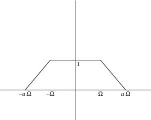
(b) Let ![]() be the function whose graph is given by Figure 2.21. Show that
be the function whose graph is given by Figure 2.21. Show that
![]()
(c) Since ![]() . Use Theorem 2.1, Theorem 2.6, and the expressions for
. Use Theorem 2.1, Theorem 2.6, and the expressions for ![]() and ga in parts a and b to show
and ga in parts a and b to show
Since ga(t) has a factor of t2 in the denominator, this expression for f(t) converges faster than the expression for f given in Theorem 2.23 (the nth tem behaves like l/n2 instead of l/n). The disadvantage of Eq. (2.29) is that the function is sampled on a grid of nπ/(aΩ) which is a more frequent rate of sampling than the grid nπ/Ω (since a > 1) used in Theorem 2.23. Thus there is a trade-off between the sample rate and the rate of convergence.
Figure 2.21. Graph of ga.