
NumPy, or Numerical Python, is a Python-based library for mathematical computations and processing arrays. Python does not support data structures in more than one dimension, with containers like lists, tuples, and dictionaries being unidimensional. The inbuilt data types and containers in Python cannot be restructured into more than one dimension, and also do not lend themselves to complex computations. These drawbacks are limitations for some of the tasks involved while analyzing data and building models, which makes arrays a vital data structure.
NumPy arrays can be reshaped and utilize the principle of vectorization (where an operation applied to the array reflects on all its elements).
In the previous chapter, we looked at the basic concepts used in descriptive data analysis. NumPy is an integral part of many of the tasks we perform in data analysis, serving as the backbone of many of the functions and data types used in Pandas. In this chapter, we understand how to create NumPy arrays using a variety of methods, combine arrays, and slice, reshape, and perform computations on them.
Getting familiar with arrays and NumPy functions
Here, we look at various methods of creating and combining arrays, along with commonly used NumPy functions.
Importing the NumPy package
The NumPy package has to be imported before its functions can be used, as shown in the following. The shorthand notation or alias for NumPy is np.
Creating an array
Methods of Creating NumPy Arrays
Method | Example |
|---|---|
Creating an array from a list | The np.array function is used to create a one-dimensional or multidimensional array from a list. CODE: np.array([[1,2,3],[4,5,6]]) Output: array([[1, 2, 3], [4, 5, 6]]) |
Creating an array from a range | The np.arange function is used to create a range of integers. CODE: np.arange(0,9) #Alternate syntax: np.arange(9) #Generates 9 equally spaced integers starting from 0 Output: array([0, 1, 2, 3, 4, 5, 6, 7, 8]) |
Creating an array of equally spaced numbers | The np.linspace function creates a given number of equally spaced values between two limits. CODE: np.linspace(1,6,5) # This generates five equally spaced values between 1 and 6 Output: array([1. , 2.25, 3.5 , 4.75, 6. ]) |
Creating an array of zeros | The np.zeros function creates an array with a given number of rows and columns, with only one value throughout the array – “0”. CODE: np.zeros((4,2)) #Creates a 4*2 array with all values as 0 Output: array([[0., 0.], [0., 0.], [0., 0.], [0., 0.]]) |
Creating an array of ones | The np.ones function is similar to the np.zeros function, the difference being that the value repeated throughout the array is “1”. CODE: np.ones((2,3)) #creates a 2*3 array with all values as 1 Output: array([[1., 1., 1.], [1., 1., 1.]]) |
Creating an array with a given value repeated throughout | The np.full function creates an array using the value specified by the user. CODE: np.full((2,2),3) #Creates a 2*2 array with all values as 3 Output: array([[3, 3], [3, 3]]) |
Creating an empty array | The np.empty function generates an array, without any particular initial value (array is randomly initialized). CODE: np.empty((2,2)) #creates a 2*2 array filled with random values Output: array([[1.31456805e-311, 9.34839993e+025], [2.15196058e-013, 2.00166813e-090]]) |
Creating an array from a repeating list | The np.repeat function creates an array from a list that is repeated a given number of times. CODE: np.repeat([1,2,3],3) #Will repeat each value in the list 3 times Output: array([1, 1, 1, 2, 2, 2, 3, 3, 3]) |
Creating an array of random integers | The randint function (from the np.random module) generates an array containing random numbers. CODE: np.random.randint(1,100,5) #Will generate an array with 5 random numbers between 1 and 100 Output: array([34, 69, 67, 3, 96]) |
One point to note is that arrays are homogeneous data structures, unlike containers (like lists, tuples, and dictionaries); that is, an array should contain items of the same data type. For example, we cannot have an array containing integers, strings, and floating-point (decimal) values together. While defining a NumPy array with items of different data types does not lead to an error while you write code, it should be avoided.
Now that we have looked at the various ways of defining an array, we look at the operations that we can perform on them, starting with the reshaping of an array.
Reshaping an array
Reshaping an array is the process of changing the dimensionality of an array. The NumPy method “reshape” is important and is commonly used to convert a 1-D array to a multidimensional one.
Consider a simple 1-D array containing ten elements, as shown in the following statement.
We can reshape the 1-D array “x” into a 2-D array with five rows and two columns:
As another example, consider the following array:
Now, apply the reshape method to create two subarrays - each with three rows and two columns:
The product of the dimensions of the reshaped array should equal the number of elements in the original array. In this case, the dimensions of the array (2,3,2) when multiplied equal 12, the number of elements in the array. If this condition is not satisfied, reshaping fails to work.
Apart from the reshape method, we can also use the shape attribute to change the shape or dimensions of an array:
Note that the shape attribute makes changes to the original array, while the reshape method does not alter the array.
The reshaping process can be reversed using the “ravel” method:
Further reading: See more on array creation routines: https://numpy.org/doc/stable/reference/routines.array-creation.html#
The logical structure of arrays
The cartesian coordinate system , which is used to specify the location of a point, consists of a plane with two perpendicular lines known as the “x” and “y” axes. The position of a point is specified using its x and y coordinates. This principle of using axes to represent different dimensions is also used in arrays.
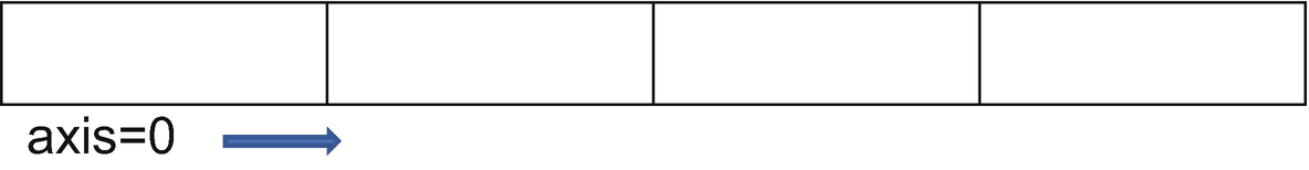
1-D array representation

A 2-D array representation

A 3-D array representation
Extending the logic, an array with “n” dimensions has “n” axes.
Note that the preceding diagrams represent only the logical structure of arrays. When it comes to storage in the memory, elements in an array occupy contiguous locations, regardless of the dimensions.
Data type of a NumPy array
The type function can be used to determine the type of a NumPy array:
Modifying arrays
The length of an array is set when you define it. Let us consider the following array, “a”:
The preceding code statement would create an array of length 3. The array length is not modifiable after this. In other words, we cannot add a new element to the array after its definition.
The following statement, where we try to add a fourth element to this array, would lead to an error:
However, you can change the value of an existing element. The following statement would work fine:
In summary, while you can modify the values of existing items in an array, you cannot add new items to it.
Now that we have seen how to define and reshape an array, we look at the ways in which we can combine arrays.
Combining arrays
- 1.
Appending involves joining one array at the end of another array. The np.append function is used to append two arrays.
CODE:x=np.array([[1,2],[3,4]])y=np.array([[6,7,8],[9,10,11]])np.append(x,y)Output:array([ 1, 2, 3, 4, 6, 7, 8, 9, 10, 11]) - 2.
Concatenation involves joining arrays along an axis (either vertical or horizontal). The np.concatenate function concatenates arrays.
CODE:x=np.array([[1,2],[3,4]])y=np.array([[6,7],[9,10]])np.concatenate((x,y))Output:array([[ 1, 2],[ 3, 4],[ 6, 7],[ 9, 10]])By default, the concatenate function joins the arrays vertically (along the “0” axis). If you want the arrays to be joined side by side, the “axis” parameter needs to be added with the value as “1”:
CODE:np.concatenate((x,y),axis=1)The append function uses the concatenate function internally.
- 3.
Stacking: Stacking can be of two types, vertical or horizontal, as explained in the following.
Vertical stacking
As the name indicates, vertical stacking stacks arrays one below the other. The number of elements in each subarray of the arrays being stacked vertically must be the same for vertical stacking to work. The np.vstack function is used for vertical stacking.
CODE:x=np.array([[1,2],[3,4]])y=np.array([[6,7],[8,9],[10,11]])np.vstack((x,y))Output:array([[ 1, 2],[ 3, 4],[ 6, 7],[ 8, 9],[10, 11]])See how there are two elements in each subarray of the arrays “x” and “y”.
Horizontal stacking
Horizontal stacking stacks arrays side by side. The number of subarrays needs to be the same for each of the arrays being horizontally stacked. The np.hstack function is used for horizontal stacking.
In the following example, we have two subarrays in each of the arrays, “x” and “y”.
CODE:x=np.array([[1,2],[3,4]])y=np.array([[6,7,8],[9,10,11]])np.hstack((x,y))Output:array([[ 1, 2, 6, 7, 8],[ 3, 4, 9, 10, 11]])
In the next section, we look at how to use logical operators to test for conditions in NumPy arrays.
Testing for conditions
NumPy uses logical operators (&,|,~), and functions like np.any, np.all, and np.where to check for conditions. The elements in the array (or their indexes) that satisfy the condition are returned.
Consider the following array:
Checking if all the values satisfy a given condition: The np.all function returns the value “True” only if the condition holds for all the items of the array, as shown in the following example.
CODE:np.all(x>20)#returns True only if all the elements are greater than 20Output:
FalseChecking if any of the values in the array satisfy a condition: The np.any function returns the value “True” if any of the items satisfy the condition.
CODE:np.any(x>20)#returns True if any one element in the array is greater than 20Output:
TrueReturning the index of the items satisfy a condition: The np.where function returns the index of the values in the array satisfying a given condition.
CODE:np.where(x<10)#returns the index of elements that are less than 10Output :
(array([0, 1], dtype=int64),)The np.where function is also useful for selectively retrieving or filtering values in an array. For example, we can retrieve those items that satisfy the condition “x<10”, using the following code statement:
CODE:x[np.where(x<10)]Output:array([1. , 6.44444444])Checking for more than one condition:
NumPy uses the following Boolean operators to combine conditions:& operator (equivalent to and operator in Python): Returns True when all conditions are satisfied:
CODE:x[(x>10) & (x<50)]#Returns all items that have a value greater than 10 and less than 50Output:array([11.88888889, 17.33333333, 22.77777778, 28.22222222, 33.66666667,39.11111111, 44.55555556])| operator (equivalent to or operator in Python): Returns True when any one condition, from a given set of conditions, is satisfied.
CODE:x[(x>10) | (x<5)]#Returns all items that have a value greater than 10 or less than 5Output:array([ 1. , 11.88888889, 17.33333333, 22.77777778, 28.22222222,33.66666667, 39.11111111, 44.55555556, 50. ])~ operator (equivalent to not operator in Python) for negating a condition.
CODE:x[~(x<8)]#Returns all items greater than 8Output:array([11.88888889, 17.33333333, 22.77777778, 28.22222222, 33.66666667,39.11111111, 44.55555556, 50. ])
We now move on to some other important concepts in NumPy like broadcasting and vectorization. We also discuss the use of arithmetic operators with NumPy arrays.
Broadcasting, vectorization, and arithmetic operations
Broadcasting
- 1.
Both the arrays have the same dimensions.
In this example, both arrays have the dimensions 2*6.
CODE:x=np.arange(0,12).reshape(2,6)y=np.arange(5,17).reshape(2,6)x*yOutput:array([[ 0, 6, 14, 24, 36, 50],[ 66, 84, 104, 126, 150, 176]]) - 2.
One of the arrays is a one-element array.
In this example, the second array has only one element.
CODE :x=np.arange(0,12).reshape(2,6)y=np.array([1])x-yOutput:array([[-1, 0, 1, 2, 3, 4],[ 5, 6, 7, 8, 9, 10]]) - 3.
An array and a scalar (a single value) are combined.
In this example, the variable y is used as a scalar value in the operation.
CODE:x=np.arange(0,12).reshape(2,6)y=2x/yOutput:array([[0. , 0.5, 1. , 1.5, 2. , 2.5],[3. , 3.5, 4. , 4.5, 5. , 5.5]])
We can add, subtract, multiply, and divide arrays using either the arithmetic operators (+/-/* and /), or the functions (np.add, np.subtract, np.multiply, and np.divide)
Similarly , you can use np.subtract (or the – operator) for subtraction, np.multiply (or the * operator) for multiplication, and np.divide (or the / operator) for division.
Further reading: See more on array broadcasting: https://numpy.org/doc/stable/user/basics.broadcasting.html
Vectorization
Using the principle of vectorization, you can also conveniently apply arithmetic operators on each object in the array, instead of iterating through the elements, which is what you would do for applying operations to items in a container like a list.
Dot product
We can obtain the dot product of two arrays, which is different from multiplying two arrays. Multiplying two arrays gives an element-wise product, while a dot product of two arrays computes the inner product of the elements.
As discussed earlier, arrays can be multiplied using the multiplication operator (*) or the np.multiply function.
The NumPy function for obtaining the dot product is np.dot.
We can also combine an array with a scalar.
In the next topic, we discuss how to obtain the various properties or attributes of an array.
Obtaining the properties of an array
Array properties like their size, dimensions, number of elements, and memory usage can be found out using attributes.
The size property gives the number of elements in the array.
CODE:
x.sizeOutput:10The ndim property gives the number of dimensions.
CODE:
x.ndimOutput:2The memory (total number of bytes) occupied by an array can be calculated using the nbytes attribute .
CODE:
x.nbytesOutput:40Each element occupies 4 bytes (since this is an int array); therefore, ten elements occupy 40 bytes
The data type of elements in this array can be calculated using the dtype attribute.
CODE:
x.dtypeOutput:dtype('int32')
Note the difference between the dtype and the type of an array. The type function gives the type of the container object (in this case, the type is ndarray), and dtype, which is an attribute, gives the type of individual items in the array.
Further reading: Learn more about the list of data types supported by NumPy:
https://numpy.org/devdocs/user/basics.types.html
Transposing an array
The transpose of an array is its mirror image.
Consider the following array:
We can use the np.transpose method.
CODE:
Alternatively, we can use the T attribute to obtain the transpose.
CODE:
Masked arrays
Let us say that you are using a NumPy array to store the scores obtained in an exam for a class of students. While you have data for most students, there are some missing values. A masked array, which is used for storing data with invalid or missing entries, is useful in such scenarios.
A masked array can be defined by creating an object of the “ma.masked_array” class (part of the numpy.ma module):
Two arrays are passed as arguments to the ma.masked_array class – one containing the values of the items in the array, and one containing the mask values. A mask value of “0” indicates that the corresponding item value is valid, and a mask value of “1” indicates that it is missing or invalid. For instance, in the preceding example, the values 87, 99, 100, and 76 are valid since they have a mask value of “0”. The last item in the first array (0), with a mask value of “1”, is invalid.
The mask values can also be defined using the mask attribute.
To unmask an element, assign it a value:
The mask value for this element changes to 1 since it is no longer invalid.
Let us now look at how to create subsets from an array.
Slicing or selecting a subset of data
Slicing of arrays is similar to the slicing of strings and lists in Python. A slice is a subset of a data structure (in this case, an array), which can represent a set of values or a single value.
Consider the following array:
Select the first subarray [0,1]:
CODE:
x[0]Output:array([0, 1])Select the second column:
CODE:x[:,1]#This will select all the rows and the 2ndcolumn (has an index of 1)Output:
array([1, 3, 5, 7, 9])Select the element at the fourth row and first column:
CODE:
x[3,0]Output:6We can also create a slice based on a condition:
CODE:
x[x<5]Output:array([0, 1, 2, 3, 4])
When we slice an array, the original array is not modified (a copy of the array is created).
Now that we have learned about creating and working with arrays, we move on to another important application of NumPy – calculation of statistical measures using various functions.
Obtaining descriptive statistics/aggregate measures
There are methods in NumPy that enable simplification of complex calculations and determination of aggregate measures.
Let us find the measures of central tendency (the mean, variance, standard deviation), sum, cumulative sum, and the maximum value for this array:
Finding out the variance:
Calculating the standard deviation:
Calculating the sum for each column:
Calculating the cumulative sum:
Finding out the maximum value in an array:
Before concluding the chapter, let us learn about matrices – another data structure supported by the NumPy package.
Matrices
A matrix is a two-dimensional data structure, while an array can consist of any number of dimensions.
With the np.matrix class, we can create a matrix object, using the following syntax:
Most of the functions that can be applied to arrays can be used on matrices as well. Matrices use some arithmetic operators that make matrix operations more intuitive. For instance, we can use the * operator to get the dot product of two matrices that replicates the functionality of the np.dot function.
Since matrices are just one specific case of arrays and might be deprecated in future releases of NumPy, it is generally preferable to use NumPy arrays.
Summary
NumPy is a library used for mathematical computations and creating data structures, called arrays, that can contain any number of dimensions.
There are multiple ways for creating an array, and arrays can also be reshaped to add more dimensions or change the existing dimensions.
Arrays support vectorization that provides a quick and intuitive method to apply arithmetic operators on all the elements of the array.
A variety of statistical and aggregate measures can be calculated using simple NumPy functions, like np.mean, np.var, np.std, and so on.
Review Exercises
Question 1
Elements in the third subarray (17,18,19,20,21,22,23,24)
Last element (24)
Elements in the second column (2,6,10,14,18,22)
Elements along the diagonal (1,10,19,24)
Question 2
An array with seven random numbers
An uninitialized 2*5 array
An array with ten equally spaced floating-point numbers between 1 and 3
A 3*3 array with all the values as 100
Question 3
Create an array to store the first 50 even numbers
Calculate the mean and standard deviation of these numbers
Reshape this array into an array with two subarrays, each with five rows and five columns
Calculate the dimensions of this reshaped array
Question 4
- 1.
Matrices
- 2.
Arrays
Question 5
What is the difference between the code written in parts 1 and 2, and how would the outputs differ?
Part 1:
Part 2:
Answers
Elements in the third subarray (17,18,19,20,21,22,23,24):
CODE:
Last element (24):
CODE:
Elements in the second column (2,6,10,14,18,22):
CODE:
Elements along the diagonal (1,10,19,24):
CODE:
An array with seven random numbers:
CODE:
An uninitialized 2*5 array:
CODE:
An array with ten equally spaced floating-point numbers between 1 and 3:
CODE:
A 3*3 array with all the values as 100:
CODE:
Question 3
Question 4
Computing the dot product using matrices requires the use of the * arithmetic operator
Computing the dot product using arrays requires the use of the dot method.
Question 5
- 1.
array([3, 6, 9])
An array supports vectorization, and thus the * operator is applied to each element.
- 2.
[1, 2, 3, 1, 2, 3, 1, 2, 3]
For a list, vectorization is not supported, and applying the * operator simply repeats the list instead of multiplying the elements by a given number. A “for” loop is required to apply an arithmetic operator on each item.