
10. The Wireless Signal
Wireless signals are an integral part of many of today's embedded system designs. Mobile computer providers talk of media convergence, where consumers will be able to browse the Internet or watch live sports on a wireless computer, mobile telephone, portable digital television, or personal digital assistant (PDA). Put simply, the media will be transparent to the wireless technology. Nevertheless, media convergence is the precursor to a myriad of complex technological issues, such as enhanced data compression, interoperability, propagation, and interference. Numerous other wireless uncertainties, such as the large number of international standards and media formats, deserve a book of their own. This chapter, in keeping with signal integrity engineering, is less concerned with media, standards, and the peculiarities of wireless propagation; it focuses on measuring and analyzing wireless signals. Wireless signals and spectrum analysis are wide-ranging subjects with several specialist areas, and it could be argued that such topics are better suited to dedicated wireless books. However, because wireless is becoming so prevalent in embedded system design and there are so many fresh wireless issues, the wireless environment deserves valuable thinking time from the signal integrity engineer. Consequently, this book would be incomplete without an explanation of modern wireless signals and their measurement. Therefore, it is the aim of this chapter to help you understand some of the new techniques in wireless signal measurement. This chapter also offers a few thought-provoking ideas about signal analysis in the modern wireless environment.
With such a rich and diverse subject as wireless signals and their measurement, it will always be debatable which wireless instruments and applications to include in a broad SI book. Nevertheless, this topic is somewhat straightforward, because it can be argued that the spectrum analyzer (SA) is the principal tool for evaluating radio frequency (RF) signal characteristics. Moreover, spectrum analysis is the dominant test setting for a wide range of wireless systems and device designs. Also, spectrum analysis currently supports research and development applications ranging from low-power radio frequency identification (RFID) systems to high-power radar and RF transmitter measurements.
10.1. Radio Frequency Signals
An RF carrier signal is like a blank piece of paper on which a message can be written and dispatched. RF carriers can transport information in many ways based on variations in the carrier's amplitude or phase, where modulation is simply a change in the shape of a wireless carrier signal. In practice, we talk of amplitude modulation (AM) and frequency modulation (FM), but to be pedantic, frequency modulation is the time derivative of phase modulation (PM). Combinations of AM and PM lead to numerous variations of modulation schemes, such as Quadrature Phase Shift Keying (QPSK), a digital modulation format in which the symbol decision points occur at multiples of 90 degrees of phase. Quadrature Amplitude Modulation (QAM) is a high-order modulation format in which both amplitude and phase are varied simultaneously to provide multiple states. Even highly complex modulation formats such as Orthogonal Frequency Division Multiplexing (OFDM) can be decomposed into magnitude and phase components. Most elementary texts on wireless provide comprehensive illustrative examples that make plain the methods used to modulate a carrier signal. In the case of understanding modulation, a picture really is worth a thousand words.
However, to understand the digital representation of a modulated wireless carrier, you must be familiar with the vector model that is commonly used to represent a signal's amplitude and phase, as shown in Figure 10-1. A signal vector can be thought of as representing the instantaneous value of the magnitude (amplitude) and phase of a signal as the length and angle of a vector, respectively. In a polar coordinate system, the same point could be expressed on a graph in traditional Cartesian coordinates, or rectangular horizontal X and vertical Y coordinates. In a digital representation of RF signals, an in-phase (I) and quadrature (Q) format of time samples are commonly used. These are mathematically equivalent to Cartesian coordinates, with I representing the horizontal or X component and Q the vertical or Y component. Figure 10-2 illustrates the magnitude and phase of a vector, along with corresponding I and Q components.
![]()
Figure 10-1. A vector model representing a signal's amplitude and phase.

Figure 10-2. A digital representation of a rotating vector with the I (in-phase) and Q (quadrature) components.

For example, consider the demodulation of an AM signal that is to be represented in I and Q components. This basically requires computing the instantaneous carrier signal magnitude for each I and Q sample, where each result is digitally represented and stored in memory. A plot of the stored data (amplitudes) over time would give a representation of the original modulating signal. However, PM demodulation is more complex and consists of computing the phase angle of I and Q samples, storing the results in memory, and performing some trigonometric computations to correct the data. Then the data is used to reconstruct the original modulating signal. Understanding quadrature I and Q signals appears difficult, but in reality it's similar to understanding the representation of the value of a sinusoid at any point in time using a vector's X and Y coordinates.
However, the ideal signals represented in Figures 10-1 and 10-2 are seldom realized in practice. As mobile telephony and various wireless systems extend throughout the modern world, a problem with radio interference emerges. Products such as mobile phones normally operate within a licensed spectrum. As a rule, manufacturers of mobile telephony equipment and other wireless devices are legally bound to operate within a specific frequency band. Such devices have to be designed to prevent the transmission of adjacent channel RF energy. This is especially challenging for complex multistandard devices that switch between different modes of transmission and maintain simultaneous links to different telephone networks. Simpler devices that operate in unlicensed frequency bands also have to be designed to function properly in the presence of interfering signals. Government regulations often dictate that these devices are allowed to transmit in only short bursts at low power levels. Accurately detecting, measuring, and analyzing "bursty"-type wireless signals are tasks of significant concern in SI engineering.
10.2. Frequency Measurement
Frequency measurements usually are made with swept spectrum analyzers. They make amplitude-versus-frequency measurements by sweeping a resolution bandwidth (RBW) filter over the frequencies of interest and recording the resultant amplitude at each frequency point. The RBW is the key measurement method for most RF measurements, where swept spectrum analyzers often provide an excellent dynamic range and highly accurate displays of a signal's static spectral components. However, the principal disadvantage of the swept spectrum analyzer is that it records amplitude data at only one frequency at a particular moment in time. This is a weakness because new RF applications are emerging with RF signals that have complex time-related characteristics. Modern RF signals, especially those in the open-access Industrial, Scientific, and Medical (ISM) band, often employ spread spectrum techniques, such as Bluetooth and WiFi, that are more intermittent or "bursty" in nature. Such short-duration wireless signals are significantly more variable in frequency than radio signals of the past. As a result, today's RF signals are more difficult to analyze with a traditional swept spectrum analyzer, which is limited in its digital modulation analysis and multidomain capabilities. Even the vector signal analyzer (VSA), which emerged to specifically address digitally modulated signals, has limited capabilities for analyzing transient signals over time in the frequency modulation domains.
Spectrum monitoring today often involves detecting elementary temporal events in the presence of nonstationary signals and uncorrelated noise. Put simply, transients, predictable and unpredictable frequency shifts, and complex modulation schemes are the norm in many of today's RF and wireless disciplines and applications. Common examples are spread-spectrum and RFID, which communicate via brief bursts of information. Although the traditional swept frequency spectrum analyzer and vector signal analyzer remain the instruments of choice for mainstream RF test and measurement applications, this chapter focuses on innovative real-time spectrum analysis (RTSA). We discuss RTSA because of the migration of today's RF applications to transient signal behavior. SI engineers now need to trigger and capture signals of interest simultaneously in the time and frequency domains. Often SI engineers need to capture a continuous record of signal fluctuations, including transients and frequency deviations, and they need to analyze the signal for changes in frequency, amplitude, and modulation. Moreover, all these operations often need to be carried out over a lengthy period of time. For example, an SI engineer could wait a significant amount of time for a swept-spectrum analyzer to detect a transient event in a modern RF system. Even then there would be a limited means of determining when the event occurred or whether the engineer had actually missed the capture of one or more events.
The common thread that runs through many emerging RF applications is the time-varying nature of the wireless signal. This characteristic, coupled with the factors already discussed, calls for a new type of analysis. As a result, SI engineers and designers are using real-time spectrum analysis in increasing numbers. Although real-time spectrum analysis is not a new concept, and it is very similar in concept to the VSA, the relevance of RTSA to SI engineering is significant. Consequently, today's SI engineer is encouraged to consider both conventional frequency-domain information and RTSA. Moreover, given the trend in SI engineering toward RTSA as more systems require simultaneous time and frequency information to reveal underlying RF signal behavior, there is a reasoned argument for focusing on RTSA in this chapter.
10.2.1. The Swept Spectrum Analyzer
The swept-tuned, superheterodyne spectrum analyzer is the traditional architecture that first enabled engineers to make frequency domain measurements several decades ago. Originally built with purely analog components, the swept SA has since evolved along with the applications it serves. Current-generation swept SAs now include advanced digital elements such as analog-to-digital conversion (ADC), digital signal processing (DSP), and microprocessors. However, the basic swept approach remains largely the same, and the instrument retains its role as the primary measurement tool for observing controlled RF signals. A clear advantage of a modern swept SA is its excellent dynamic range, whereby it can capture and detect a broad array of RF data.
The swept SA makes power-versus-frequency measurements by down-converting the signal of interest and sweeping it through the passband of an RBW filter. The RBW filter is followed by a detector that calculates the amplitude at each frequency point in the selected passband, as shown in Figure 10-3.
Figure 10-3. A block diagram of a traditional RBW spectrum analyzer.

Figure 10-3 shows the measurement trade-off between frequency resolution and time. The local oscillator sweeps through a "span" of frequencies feeding the mixer. Each sweep produces sum and difference frequencies at the mixer output. The resolution filter has a bandwidth that is set to a user-selected frequency, the RBW. The narrower the filter bandwidth, the higher the resolution of the measurement, and the greater the exclusion of unwanted instrument-generated noise. The RBW filter feeds the detector, which measures the spectral power at each instant in time to produce a frequency-domain display plotting spectral power against frequency. While this method can provide high dynamic range, its principal disadvantage is that it can calculate the amplitude data for only one frequency point at a time. If the RBW filters are made too narrow, the time taken to complete a sweep of the RF input is too long, and any changes in the RF input go undetected. Sweeping the analyzer over a span of frequencies or number of passbands can take considerable time. This measurement technique is based on the assumption that the analyzer can complete several sweeps without any significant changes to the signal being measured. Consequently, a relatively stable, unchanging input signal is required. If the signal changes rapidly, the change probably will be missed.
For example, the left part of Figure 10-4 shows an RBW logic analyzer sweep that is looking at frequency segment Fa while a momentary spectral event occurs at Fb. By the time the sweep arrives at segment Fb, the event has vanished and goes undetected. The RBW spectrum analyzer sweep fails to provide a trigger for the transient signal at Fb and fails to store a comprehensive record of signal behavior over time. This is an example of the classic trade-off between frequency resolution and measurement time, which is the Achilles' heel of the traditional RBW spectrum analyzer.
Figure 10-4. The sweep on the left is looking at frequency segment Fa while a momentary spectral event occurs at Fb. The right side of the figure shows the Fb measurement taking place, with the missing transient.
However, a modern swept SA is significantly faster than its traditional purely analog predecessor. Figure 10-5 shows a classic modern swept SA architecture. Traditional wide analog RBW filters have been enhanced with digital techniques to facilitate fast and accurate narrower band filtering. Nevertheless, the filtering, mixing, and amplification preceding the ADC are analog processes. When exacting narrow band-pass filters are needed, they are implemented by DSP in the stage following the ADC. However, the job of the ADC and DSP is rather demanding. In particular, nonlinearity and noise in the ADC can be a concern, and there remains a place for the analog spectrum analyzer, which is an ideal tool for eliminating these problems.
Figure 10-5. A modern swept SA architecture with digital circuitry.

10.2.2. The Vector Signal Analyzer
Traditional swept spectrum analysis enables scalar measurements to provide information about the magnitude of each frequency component in an input signal. Analyzing signals that carry digital modulation requires a vector measurement to provide both magnitude and phase information about the input signal. The vector signal analyzer is a tool specifically designed for digital modulation analysis. Figure 10-6 shows a simplified VSA block diagram, where the VSA is optimized for modulation measurements.
Figure 10-6. A simplified block diagram of the VSA.
Like the Real-Time Spectrum Analyzer (RTSA) described in the next section, a VSA digitizes all the RF energy within the instrument's passband to extract the magnitude and phase information required for digital modulation measurements. However, most, but not all, VSAs are designed to take snapshots of the input signal at arbitrary points in time. This makes it difficult or impossible to store a long record of successive acquisitions for a cumulative history of how a signal behaves over time. Like a swept SA, the triggering capabilities typically are limited to an intermediate frequency (IF) level trigger and an external trigger.
Within the VSA, an ADC digitizes the wideband IF signal, and then the down-conversion, filtering, and detection are performed numerically. The transformation from the time domain to the frequency domain is processed by Fast Fourier Transform (FFT) algorithms. The linearity and dynamic range of the ADC are critical to the instrument's performance. Equally important, there must be sufficient DSP power to enable fast measurements. Nonetheless, some VSAs have significant measurement capabilities and can provide a detailed analysis of RF signal behavior.
The VSA typically measures modulation parameters such as error vector magnitude (EVM) and provides other displays, such as a constellation diagram. A stand-alone VSA is often used to supplement the capabilities of a traditional swept SA. In addition, many modern instruments have architectures that can perform both swept SA and VSA functions. These instruments provide frequency and modulation domain measurements within one instrument; however, both measurements are not always correlated in time.
10.3. Overview of the Real-Time Spectrum Analyzer
The RTSA is designed to capture and analyze RF signals that have transient and dynamic characteristics. The fundamental concept of real-time spectrum analysis is to trigger on an RF signal event, seamlessly capture the digitized data into memory, and then provide a built-in analysis of the data in multiple domains. Figure 10-7 is a simplified block diagram of the RTSA architecture. The RF front end can be tuned across the instrument's entire frequency range, and it down-converts the RF input signal to a fixed IF that is related to the RTSA's maximum real-time bandwidth. The signal is then filtered, digitized by the ADC, and passed to the DSP engine that manages the instrument's triggering, memory, and analysis functions.
Figure 10-7. A simplified block diagram of the RTSA architecture.
While elements of the RTSA block diagram and acquisition process are similar to those of the VSA architecture, the RTSA is optimized to deliver real-time triggering, seamless signal capture, and time-correlated multidomain analysis. An important consideration for the RTSA is the need to incorporate advanced ADC technology to enable a conversion with high dynamic range and low noise for the measurement to be comparable to a swept SA. For measurement spans that are less than or equal to the instrument's real-time passband, the RTSA architecture lets you seamlessly capture the input signal with no gaps in time by digitizing the RF signal and storing the time-contiguous samples in memory. RTSA has several advantages over the acquisition process of a swept spectrum analyzer for measuring modern "bursty" wireless signals. This makes it an exciting modern instrument to discover and is why RTSA is the focus of this chapter. Nonetheless, the SI engineer must bear in mind that the classic RBW spectrum analyzer remains the instrument of choice for a significant number of RF measurements.
10.3.1. Fast Fourier Transform Analysis
The Fast Fourier Transform is at the heart of real-time spectrum analysis. In the RTSA, FFT algorithms are employed to transform time-domain signals into their frequency-domain spectral components. Conceptually, FFT processing can be considered as passing an RF signal through a bank of parallel filters where each filter has an equal frequency resolution and bandwidth but detects a different component. The FFT output generally is complex-valued, which means that it represents each frequency component as a vector with a particular phase and magnitude. For spectrum analysis, the amplitude of the complex component is usually of most interest.
The FFT process starts with properly decimated and filtered baseband I and Q components, which form the complex representation of the signal, with I as its real part and Q as its imaginary part. In FFT processing, a set of samples of the complex I and Q signals are processed at the same time. This set of samples is called the FFT frame. The number of samples in the FFT, generally a power of 2, is also called the FFT size. For example, a 1,024-point FFT can transform 1,024 I samples and 1,024 Q samples into 1,024 complex frequency-domain points.
10.3.1.1. FFT Properties
A lot of jargon is associated with an FFT, which can obscure the simple concepts of an FFT process. Put simply, the amount of time required to acquire a set of samples upon which an FFT is performed is called the frame length. The frame length in the RSA is the product of the FFT size and the sample period; it's the time taken to perform a single measurement. Any changes, or temporal events, that occur in the measured signal during the frame length cannot be resolved. Therefore, the frame length is simply the time resolution of the FFT process or a single measurement period for an RTSA. The frequency domain points of FFT processing are often called FFT bins. Therefore, the FFT size is equal to the number of bins in one FFT frame. Those bins are equivalent to the individual filter output of an RTSA parallel filter. All bins are spaced equally in frequency. Two spectral lines closer than the bin width cannot be resolved. The FFT frequency resolution therefore is the width of each frequency bin, which is equal to the sample frequency divided by the FFT size. Therefore, for the same sample rate, a larger FFT size yields a finer frequency resolution. For example, an RTSA with a sample rate of 25.6 MHz and an FFT size of 1,024 gives a frequency resolution of 25 kHz.
Frequency resolution can be improved by increasing the FFT size or by reducing the sampling frequency. The RTSA typically uses a digital down-converter (DDC) and decimator to reduce the effective sampling rate as the frequency span is narrowed. This effectively trades time resolution for frequency resolution while keeping the FFT size and computational complexity at manageable levels. This approach allows fine resolution on narrow spans without excessive computation time on wide spans, where coarser frequency resolution is sufficient. The practical limit on FFT size is often display resolution, because an FFT with resolution much higher than the number of display points does not provide any additional information on the instrument's screen.
10.3.2. Windowing
An assumption inherent in the mathematics of Discrete Fourier Transforms (DFTs) and FFT analysis says that the data to be processed is a single period of a periodically repeating signal. Figure 10-8 depicts the FFT of a series of time domain frames. For example, when FFT processing is applied to Frame 2, the transform process assumes that the signal is periodic. However, the process generally produces discontinuities between successive frames, as shown in Figure 10-9. These artificial discontinuities generate spurious responses not present in the original signal, which can make it impossible to detect small signals in the presence of nearby large ones. This effect is called spectral leakage.
Figure 10-8. Three frames of a sampled time domain signal.

Figure 10-9. Discontinuities between frames.

Typically an RSA applies a windowing technique to the FFT frame before FFT processing is performed to reduce the effects of spectral leakage. The window functions usually have a bell shape. Numerous window functions are available. Figure 10-10 shows the popular Blackman-Harris 4B (BH4B) profile. The Blackman-Harris 4B windowing function shown in Figure 10-10 has a value of 0 for the first and last samples and a continuous curve in between. Multiplying the FFT frame by the window function reduces the discontinuities at the ends of the frame. In the case of the Blackman-Harris window, we can eliminate discontinuities. The effect of windowing is to place a greater weight on the samples in the center of the window than those away from the center, bringing the value to 0 at the ends. This can be thought of as effectively reducing the time over which the FFT is calculated. It should be noted that time and frequency are reciprocal quantities and a smaller time sample implies poorer (wider) frequency resolution. For Blackman-Harris 4B windows, the effective frequency resolution is approximately twice as wide as the value achieved without windowing.
Figure 10-10. A BH4B window profile.
Another implication of windowing is that the time-domain data modified by this window produces an FFT output spectrum that is most sensitive to behavior in the center of the frame and is insensitive to behavior at the beginning and end of the frame. Transient signals appearing close to either end of the FFT frame are de-emphasized and can be missed. This problem can be resolved by using overlapping frames, a complex technique involving trade-offs between computation time and time-domain flatness to achieve the desired performance.
10.3.3. Key Concepts of Real-Time Spectrum Analysis
As you have seen, the measurements performed by an RTSA are implemented using DSP techniques. To understand how an RF signal can be analyzed in the time, frequency, and modulation domains, first you must examine how the instrument acquires and stores a signal. After the ADC digitizes an RF input, the signal is represented by time domain data, from which all frequency and modulation parameters can be calculated using DSP. Three terms samples, frames, and blocks describe the hierarchy of data stored when an RTSA contiguously captures a signal using real-time acquisition. Figure 10-11 illustrates the sample-frame-block structure.
Figure 10-11. The sample-frame-block structure of an RTSA acquisition.
The lowest level of the data hierarchy is the sample, which represents a discrete time-domain data point. This construct is familiar from other applications of digital sampling, such as real-time oscilloscopes and PC-based digitizers. The effective sample rate that determines the time interval between adjacent samples depends on the selected span. In the RTSA, each sample is stored in memory as an IQ pair, where I is the signal's in-phase magnitude component and Q is the signal's quadrature component.
The next in the hierarchy is the frame. A frame consists of an integer number of contiguous samples and is the basic unit to which the FFT can be applied to convert time domain data into the frequency domain. In this process, each frame yields one frequency domain spectrum.
The highest level in the acquisition hierarchy is the block, which is made up of many adjacent frames that are captured seamlessly in time. The block length, also called the acquisition length, is the total amount of time that is represented by one continuous acquisition. Within a block, the input signal is represented with no gaps in time.
In the real-time measurement modes of the RTSA, each block is seamlessly acquired and stored in memory. It is then post-processed using DSP techniques to analyze the signal's frequency, time, and modulation behavior. In standard SA modes, the RTSA can emulate a swept SA by stepping the RF front end across frequency spans that exceed the maximum real-time bandwidth. Figure 10-12 shows block acquisition mode. Although each acquisition is seamless in time for all the frames within a block, remember that data capture is not contiguous between blocks.
Figure 10-12. RTSA block acquisition mode.

After the signal processing of one acquisition block is complete, the next block is acquired. As soon as the block is stored in memory, real-time measurements can be applied. For example, a signal captured in real-time SA mode can then be analyzed in demodulation mode and time mode. The number of frames acquired within a block can be determined by dividing the acquisition length by the frame length. Normally the user enters the acquisition length; it is rounded so that the block contains an integer number of frames. The maximum acquisition length ranges from seconds to days. It is limited by the selected measurement span and the instrument's memory depth.
10.4. How a Real-Time Spectrum Analyzer Works
A modern real-time spectrum analyzer can acquire a passband, or span, anywhere within the analyzer's input frequency range. At the heart of this capability is an RF down-converter followed by a wideband IF section. An ADC digitizes the IF signal, and the system performs all further steps digitally. An FFT algorithm implements the transformation from time domain to frequency domain, where subsequent analysis produces displays such as spectrograms, codograms, and more.
Several key characteristics distinguish a successful real-time architecture:
• An ADC system that can digitize the entire real-time bandwidth with sufficient fidelity to support the desired measurements.
• An integrated signal analysis system that provides multiple analysis views of the signal under test, all correlated in time.
• Sufficient capture memory and DSP power to enable continuous real-time acquisition over the desired time measurement period.
• DSP power to enable real-time triggering in the frequency domain.
This section contains several architectural diagrams of the main acquisition and analysis blocks of a proprietary RTSA. The principles of operation that are described typically apply to real-time spectrum analysis in general. However, some ancillary functions, such as minor triggering-related blocks and display and keyboard controllers, have been omitted to clarify the discussion.
10.4.1. Digital Signal Processing in Real-Time Spectrum Analysis
A modern RSA uses a combination of analog and digital signal processing to convert RF signals into calibrated, time-correlated multidomain measurements. This section deals with the digital portion of the RSA signal processing flow. Figure 10-13 illustrates the major digital signal processing blocks used in a modern RSA. An analog IF signal is band-pass filtered and digitized. A digital down-conversion and decimation process converts the analog to digital converted samples into streams of in-phase (I) and quadrature (Q) baseband signals. A triggering block detects signal conditions to control acquisition and timing. The baseband I and Q signals as well as triggering information are used by a baseband DSP system to perform spectrum analysis by means of FFT, modulation analysis, power measurements, timing measurements, and statistical analysis.
Figure 10-13. The major digital signal processing blocks used in a modern RSA.

10.4.2. IF Digitizer
An RSA typically digitizes a band of frequencies centered on an IF. This band or span of frequencies is the widest frequency for which real-time analysis can be performed. Digitizing at a high IF rather than at DC or baseband has several signal processing advantages, such as overcoming spurious performance, DC rejection, and improved dynamic range. But this can result in excessive computation to filter and analyze the data if processed directly. An alternative technique, shown in Figure 10-13, is to employ a DDC and a decimator to convert the digitized IF into I and Q baseband signals at an effective sampling rate just high enough for the selected span.
10.4.3. Digital Down-Converter
As shown in Figure 10-13, the IF signal in an RSA is digitized with a sampling rate designated as FS. The digitized IF is then sent to a DDC. A numeric oscillator in the DDC generates sine and cosine signals at the centered frequency of the band of interest. The sine and cosine signals are numerically multiplied with the digitized IF to generate streams of I and Q baseband samples that contain all the information present in the original IF signal. The I and Q streams then pass through variable-bandwidth low-pass filters where the cut-off frequency of the low-pass filters is varied according to the selected span.
10.4.4. I and Q Baseband Signals
Figure 10-14 illustrates the process of taking a frequency band and converting it to baseband using quadrature down-conversion. The original IF signal is contained in the space between three halves of the sampling frequency and the sampling frequency itself.
Figure 10-14. Information in the passband is maintained in I and Q at half the sample rate.
Sampling produces an image of this signal between zero and one-half the sampling frequency. The signal is then multiplied with coherent sine and cosine signals at the center of the passband of interest, generating I and Q baseband signals. The baseband signals are real-valued and symmetric about the origin. The same information is contained in each so-called sideband; therefore, it is possible to decimate by 2.
10.4.5. Decimation
The Nyquist theorem states that for baseband signals, you only need to sample at a rate equal to twice the highest frequency of interest. Remembering that time and frequency are reciprocal quantities, it is evident that to study low frequencies with an RSA, you must observe a long time record. For this reason, among others, decimation is used to balance span, processing time, record length, and memory usage.
Consider a practical example. An RTSA uses a 51.2 million samples per second (MSs-1) sampling rate at an ADC to digitize a span of 15 MHz bandwidth. Then the I and Q records that result after DDC, filtering, and decimation for the 15 MHz span are at an effective sampling rate of half the original sample rate, which is 25.6 MSs-1. The total number of samples is unchanged, but we are left with two sets of samples, each at an effective rate of 25.6 MSs-1 instead of a single set at 51.2 MSs-1.
Further decimation can be made for narrower spans, resulting in longer time records for an equivalent number of samples. The disadvantage of the lower effective sampling rate is a reduced time resolution. The advantages of the lower effective sampling rate are fewer computations and less memory usage for a given time record, as shown in Table 10-1.
Table 10-1. Examples of Selected Span, Decimation, and Effective Sample Rates
10.4.6. Time and Frequency Domain Effects on the Sampling Rate
Using decimation to reduce the effective sampling rate has several consequences for important time and frequency domain measurement parameters. Figures 10-15 and 10-16 show an example contrasting a wide span and a narrow span. A wide-capture bandwidth displays a broad span of frequencies with relatively low frequency domain resolution. Compared to narrower-capture bandwidths, the sample rate is higher, and the resolution bandwidth is wider. In the time domain, frame length is shorter, and time resolution is finer. Record length is the same in terms of the number of stored samples, but the amount of time represented by these samples is shorter.
Figure 10-15. Wide bandwidth capture.

Figure 10-16. Narrow bandwidth capture.
In contrast, a narrow-capture bandwidth displays a small span of frequencies with higher frequency domain resolution. In a wide-capture bandwidth, the sample rate is lower and the frequency domain resolution is lower. In the time domain, the frame length is longer and the time resolution is coarser, although the available record length encompasses more time. This can be seen in Figure 10-15, which illustrates a narrow bandwidth capture. Table 10-1 provides some real-world examples. It is important to note the scale of the numbers such as frequency resolution, which are several orders of magnitude different from the wideband capture. This is significant when you're using an RSA.
10.5. Applying Real-Time Spectrum Analysis
Real-time spectrum analysis adds the time domain to spectrum and modulation analysis. Triggering is critical to capturing time domain information, and trigger functionality provides the ability to detect and correct signal integrity errors in common with the oscilloscope and logic analyzer. The most common trigger system used in benchtop instrumentation is the one found in most oscilloscopes. In traditional analog oscilloscopes, the signal to be observed is connected to one input, and the trigger is connected to another, or the trigger is extracted from the captured signal. The trigger event causes the start of a horizontal sweep. The signal's amplitude is shown as a vertical displacement superimposed on a calibrated graticule. In its simplest form, analog triggering allows events that happen after the trigger point to be observed, as shown in Figure 10-17.
Figure 10-17. Traditional oscilloscope triggering.
The ability to represent and process signals digitally and with a large memory capacity allows the capture of events before and after the trigger point. Digital acquisition systems of the type used in a typical RSA use an ADC to fill a deep memory with time samples of the received signal. Conceptually, new samples are continuously fed to the memory while the oldest samples fall off. Figure 10-18 shows a memory configured to store N samples. The arrival of a trigger stops the acquisition, freezing the contents of the memory. The addition of a variable delay in the path of the trigger signal allows events that happen before a trigger as well as those that come after it to be captured.
Figure 10-18. Triggering in digital acquisition systems.
Consider a case in which there is no delay. The trigger event causes the memory to freeze immediately at the trigger point and store a sample concurrent with the trigger point. The memory then contains the sample at the time of the trigger, as well as N samples that occurred before the trigger. Only pre-trigger events are stored. Now consider the case in which the delay is set to match exactly the memory's length. N samples are then allowed to come into the memory after the trigger occurrence before the memory is frozen. The memory now contains N samples of signal activity after the trigger. Only post-trigger events are stored. Both post- and pre-trigger events can be captured if the delay is set to a fraction of the memory length. If the delay is set to half of the memory depth, half of the stored samples are those that preceded the trigger and half of the stored samples that followed it. This concept is similar to a trigger delay used in the zero span mode of a conventional swept SA. However, an RSA typically can capture much longer time records; this signal data can subsequently be analyzed in the frequency, time, and modulation domains. This is an important measurement technique for applications that require signal monitoring and SI troubleshooting.
10.5.1. RTSA Trigger Sources and Data-Capture Techniques
An RTSA normally provides several methods of internal and external triggering. Various real-time trigger sources exist. Each is suited to a particular application, setting, and required time resolution:
• External triggering typically allows an external transistor-transistor logic (TTL) signal to control data acquisition. This is usually a control signal such as a frequency switching command from the system under test. This external signal prompts the acquisition of an event in the system under test.
• Internal triggering depends on the characteristics of the signal being tested. An RSA normally can trigger on the level or amplitude of the digitized signal, on the power of the signal after filtering and decimation, or on the occurrence of specific spectral components using a frequency mask trigger.
Each of the trigger sources and modes offers specific advantages in terms of frequency selectivity, time resolution, and dynamic range. The functional elements that support these features are shown in Figure 10-19. Level triggering compares the digitized signal at the output of the ADC with a user-selected setting. The full bandwidth of the digitized signal is used, even when observing narrow spans that require further filtering and decimation. Level triggering uses the full digitization rate and can detect events with durations as brief as one sample at the full sampling rate. The time resolution of the downstream analyses, however, is limited to the decimated effective sampling rate. The trigger level is set as a percentage of the ADC clip level—that is, its maximum binary value, all 1s. This is a linear quantity not to be confused with the logarithmic display, which is expressed in dB.
Figure 10-19. A simplified block diagram of a digital SA trigger processing system.
Power triggering calculates the power of the signal after filtering and decimation. The power of each filtered pair of I and Q samples (I2 + Q2) is compared with a user-selected power setting. The setting is in dB relative to full scale (dBfs), as shown on the logarithmic display screen. A setting of 0 dBfs places the trigger level at the top graticule of the display and generates a trigger when the total power contained in the span exceeds that trigger level. Likewise, a setting of -10 dBfs triggers when the total power in the span reaches a level 10 dB below the display's top graticule. It should be noted that the total power in the span generates a trigger. For example, two carrier wave signals, each at a level of -3 dBm, would have an aggregate power of 0 dBm.
Frequency mask triggering compares the spectrum shape to a user-defined mask. This technique allows changes in a spectrum shape to trigger an acquisition. Frequency mask triggers typically are used to detect signals that are significantly below full-scale measurement, even in the presence of other signals at much higher levels. This ability to trigger on weak signals in the presence of strong ones is critical for detecting intermittent signals in the presence of intermodulation products and transient spectrum containment violations. However, a full FFT is required to compare a signal to a mask, and this takes a complete frame. Therefore, the time resolution for a frequency mask trigger is roughly one FFT frame, typically 1,024 samples at the effective sampling rate. Trigger events normally are determined in the frequency domain using a dedicated hardware FFT processor, as shown in Figure 10-19.
10.5.2. Constructing a Frequency Mask
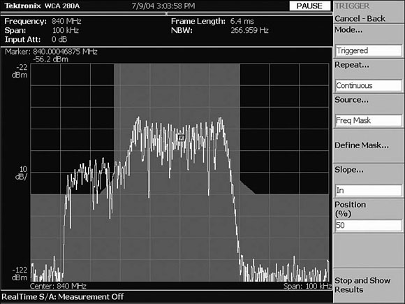
Like other forms of mask testing in oscilloscopes and logic analyzers, the RSA frequency mask trigger, also called the frequency domain trigger, starts with a definition of an on-screen mask. The mask typically is defined with a set of frequency points and their amplitudes. The mask normally is defined point by point or graphically by drawing it with a mouse or other computer pointing device. Triggers generally are set to occur when a signal outside the mask boundary "breaks in" or when a signal inside the mask boundary "breaks out." Figure 10-20 shows a frequency mask defined to allow the passage of a signal's normal spectrum but not momentary aberrations. Figure 10-21 shows a spectrogram display for an acquisition that was triggered when the signal momentarily exceeded the mask.
Figure 10-20. A frequency mask definition.
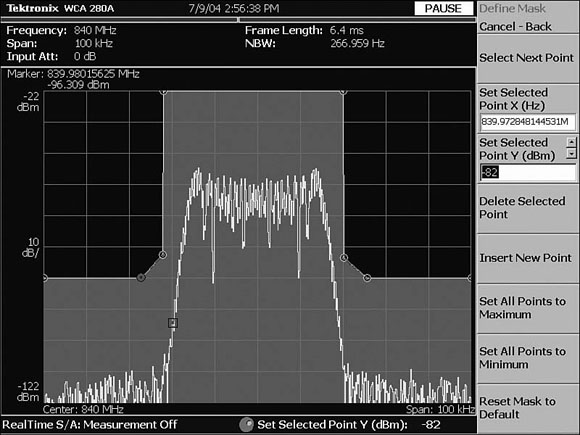
Figure 10-21. An acquisition that was triggered when the signal momentarily exceeded the frequency mask.
10.5.3. Frequency Domain Measurements
Real-time spectrum analysis lets you analyze captured time domain data using a power-versus-frequency spectrogram display. A spectrogram has three axes:
• The horizontal axis represents frequency.
• The vertical axis represents time.
• The gray scale or color represents amplitude.
The spectrogram is an important measurement that provides an intuitive display of how frequency and amplitude behavior change over time. Figure 10-22 shows the spectrogram of a dynamic signal. The horizontal axis represents the same range of frequencies that a traditional spectrum analyzer shows on the power-versus-frequency display. In the spectrogram, the vertical axis represents time, and amplitude is represented by the trace's gray scale or color. In an RTSA, each "slice" of the spectrogram corresponds to a single frequency spectrum calculated from one frame of captured time domain data. Figure 10-23 shows the power-versus-frequency and spectrogram displays for the signal shown in the figure. On the spectrogram, the oldest frame is shown at the top of the display, and the most recent frame is shown at the bottom. This measurement shows an RF signal whose frequency is changing over time. It also reveals a low-level transient signal that appears and disappears near the end of the time block. Since the data is stored in memory, a marker can be used to scroll "back in time" through the spectrogram. In Figure 10-23 a marker has been placed on the transient event on the spectrogram display. This causes the spectrum corresponding to that particular point in time to be shown on the power-versus-frequency display.
Figure 10-22. A real-time spectrogram dynamic signal.

Figure 10-23. A time-correlated view of a power-versus-frequency display, shown on the left, and the corresponding spectrogram display, shown on the right.

When combined with real-time triggering capabilities, the spectrogram becomes a more useful measurement, especially for dynamic RF signals, as shown in Figures 10-24 and 10-25. However, the SI engineer must remember a few key points when using a spectrogram display:
• Frame time is span-dependent; a wider span equals a shorter time.
• One vertical step-through of the spectrogram equals one real-time frame.
• One real-time frame equals 1,024 time domain samples.
• The oldest frame is at the top of the screen; the most recent frame is at the bottom.
• The data within a block is contiguous in time.
• Horizontal black lines on the spectrogram represent boundaries between blocks; these are the gaps in time that occur between acquisitions.
• The white bar on the left side of a spectrogram display denotes post-trigger data.
Figure 10-24. Real-Time SA mode showing a spectrogram of a frequency-hopping signal.
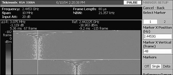
Figure 10-25. Real-Time SA mode showing several blocks acquired using a frequency mask trigger to measure the repeatability of frequency switching transients.

10.5.4. Time Domain Measurements
The frequency-versus-time measurement displays frequency on the vertical axis and time on the horizontal axis. It provides a result similar to what is shown on the spectrogram display, with two important differences. First, the frequency-versus-time view has much better time domain resolution than the spectrogram. Second, this measurement calculates a single average frequency value for every point in time, which means that it is unable to display multiple RF signals like the spectrogram. The spectrogram is a compilation of frames and has a line-by-line time resolution equal to the length of one frame. In contrast, the frequency-versus-time view has a time resolution of one sample interval. For example, if a frame has 1,024 samples, the resolution of the frequency-versus-time measurement would be 1,024 times finer than that of a spectrogram. This makes it easy for a frequency-versus-time measurement to show small or short frequency shifts in greater detail. The frequency-versus-time measurement acts almost like a very fast frequency counter, where each of the 1,024 sample points represents a frequency value, whether the span is a few hundred hertz or many megahertz. Constant-frequency signals such as a carrier wave or amplitude modulation produce a flat, level display.
The frequency-versus-time view provides the best results when there is a relatively strong signal at one unique frequency. Figure 10-26 is a simplified illustration contrasting the frequency-versus-time display with a spectrogram. The frequency-versus-time display is in some ways a zoomed-in view that magnifies a portion of the spectrogram. This is very useful for examining transient events such as frequency overshoot or ringing. When there are multiple signals in the measured environment, or one signal with an elevated noise level, or intermittent spurs, the spectrogram remains the preferred view. Put simply, it provides a visualization of all the frequency and amplitude activity across the chosen span.
Figure 10-26. A comparison of spectrogram and frequency-versus-time views.
Figures 10-27, 10-28, and 10-29 compare the frequency-versus-time and spectrogram displays by showing three different analyses or views of the same acquisition. In Figure 10-27, the frequency mask trigger was used to capture a transient signal coming from a transmitter having occasional problems with frequency stability during turn-on. Since the oscillator was not tuned to the frequency at the center of the screen, the RF signal broke the frequency mask, as shown on the left of Figure 10-27, and caused a trigger. The spectrogram plot on the right of Figure 10-27 shows a 35 ms time segment of the device's frequency settling behavior.
Figure 10-27. A spectrogram showing a 5 MHz signal settling over 35 ms of time.
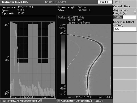
Figure 10-28. A frequency-versus-time view of the frequency settling behavior of the 5 MHz signal over 25 ms of time.
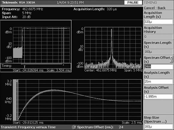
Figure 10-29. The same 5 MHz signal with a zoomed-in view to give a 50 kHz frequency versus 1 ms time display of the signal's settling behavior.

The next two figures show frequency-versus-time displays of the same signal. Figure 10-28 shows the same frequency settling behavior of the 5 MHz signal from Figure 10-27, but the frequency-versus-time display allows a shorter 25 ms analysis length. Figure 10-29 shows that you can zoom in to a frequency-versus-time display to give an analysis length of 1 ms, which shows the changes in frequency over time with a much finer time domain resolution. This reveals a residual oscillation on the signal even after it has settled to the correct frequency.
Another time-domain measurement is the magnitude of both I and Q as a function of time. The amplitude-versus-time measurement shows the raw I and Q output signals coming from the digital down-converter. This measurement is a useful troubleshooting tool for expert users, especially in terms of providing insight into irregular frequencies, phase errors, and instabilities.
10.5.5. Power Measurements
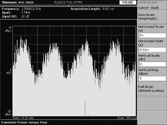
A power-versus-time measurement shows how a signal's power changes on a sample-by-sample basis. This is shown in Figure 10-30, where the signal's amplitude is plotted in dBm on a logarithmic scale. The power-versus-time display is similar to an oscilloscope time-domain view in that the horizontal axis represents time. However, in contrast to an oscilloscope display, the vertical axis of a power-versus-time display shows power on a logarithmic scale instead of voltage on a linear scale. In addition, the power-versus-time display gives a measurement that represents the total power detected within the measurement span. For example, a constant power signal yields a flat trace display because there is no average power change per cycle. For each time domain sample point, a signal's logarithmic power ratio is calculated with reference to a 1mW signal, as shown in Equation 10-1.
Equation 10-1
![]()
Figure 10-30. A power-versus-time display.

10.5.6. Complementary Cumulative Distribution Measurements
An experienced SI engineer typically uses the Complementary Cumulative Distribution Function (CCDF) measurement to determine the probability of a peak power signal component exceeding the average power of a measured signal. In other words, it displays the percentage probability that a part of the signal will momentarily exceed the average power amplitude that is displayed on the horizontal scale. The probability is displayed as a percentage value on the vertical scale, where the vertical axis is a logarithmic scale.
CCDF analysis actually measures the time-varying crest factor, which is an important measurement for many digital signals, especially those that use Code Division Multiple Access (CDMA) and Orthogonal Frequency Division Multiplexing (OFDM). The crest factor measurement is the calculated ratio of a signal's peak voltage divided by its average voltage with the result expressed in dB, as shown in Equation 10-2.
Equation 10-2
![]()
The signal's crest factor determines how linear a transmitter or receiver must be to avoid unacceptable levels of signal distortion. The CCDF curves in Figure 10-31 show the measured signal against a Gaussian reference trace. The CCDF and crest factor measurements are especially interesting to designers, because they must balance power consumption and distortion performance of devices such as RF amplifiers.
Figure 10-31. A CCDF measurement.
10.5.7. Modulation Domain Measurements
Apart from signal capture and automated measurement, the trend today is for a modern instrument to automatically analyze the captured signal. In the case of the RTSA, the instrument provides automated demodulation analysis of amplitude modulation, frequency modulation, and phase modulation. Just like time domain measurements, these analytical tools are based on the concept of multidomain analysis.
The digital demodulation mode can demodulate and analyze many common digital signals based on phase shift keying (PSK), frequency shift keying (FSK), and QAM. An RSA typically provides a wide range of measurements, including constellation, error vector magnitude (EVM), magnitude error and phase error, demodulated IQ versus time, symbol table, and eye diagrams. The SI engineer has to properly configure the instrument to enable accurate demodulation measurements and a number of variables such as the modulation type, symbol rate, and measurement filter types. This is a complex task that requires patience and practice. However, today's instruments, such as VSAs and RTSAs, provide built-in modulation measurements and analysis for many communications standards. Figure 10-32 shows the modulation analysis of a Wideband Code Division Multiple Access (W-CDMA) mobile telephone handset signal that is under closed-loop power control. The lower-right constellation display shows the error associated with large glitches that occur during level transitions. The transitions can be seen in the upper-left correlated power-versus-time display.
Figure 10-32. Modulation analysis of a W-CDMA handset under closed-loop power control. The lower right is a constellation display, and the upper left is a correlated power-versus-time measurement.

10.5.8. The Codogram Display
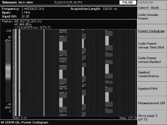
Modern mobile telephony provides voice, text messaging, and data communication, often including Internet access. Such systems naturally make use of complex modulation and signaling techniques that require complex measurement and analysis. The codogram illustrated in Figure 10-33 adds a time axis to code domain power measurements for the complex CDMA-based communications standards. Like the spectrogram, the codogram intuitively shows changes over time. Figure 10-34 is an actual W-CDMA codogram display showing a simulated W-CDMA compressed mode handoff in which the data rate is momentarily increased to make room for temporary dual-mode operations.
Figure 10-33. The codogram display.

Figure 10-34. A codogram measurement of a W-CDMA signal.
10.5.9. Jitter Measurements
Interestingly, the spectrum analyzer is a key instrument for measuring and testing bound RF signals. A case in point is the signal integrity of the new high-speed serial buses. An RF digital signal in the GHz region is bound to a printed circuit board and, unlike a wireless signal, its electromagnetic radiation is deliberately kept to a minimum. A primary measurement is random jitter and maximum periodic jitter or deterministic jitter, which you need to consider when evaluating a new high-speed serial bus design. Nonetheless, radio signals, particularly wireless data, often require jitter analysis.
Combined with a precise frequency source, an RF signal can be translated to a lower frequency to allow minute changes in signal phase to be accurately measured with a spectrum analyzer. After you measure signal phase deviation, a direct conversion to time is possible where, for example, a signal that changes phase by 1 degree has a 1/360 change in period. When jitter is measured with a spectrum analyzer, it is called phase noise and is measured relative to the correct signal in dBc. The signal under test is considered the fundamental frequency or carrier frequency. Its phase noise results are normalized to a unit Hertz value based on several aspects of the spectrum analyzer measurement system, such as filter bandwidths and sweep rates. The advantage of using a spectrum analyzer for a jitter measurement is that normally there is a very good phase measurement resolution, and the instruments themselves typically have very low noise floors. This provides a platform that can measure frequency and phase change well below what is possible in conventional time-domain instrumentation. For example, several common spectrum analyzers have noise floors below -105 dB at a 10 kHz offset. This is compared to a current real-time oscilloscope, which comes in with -50 dB at a 10 kHz offset. Spectrum analyzers can be quite effective at finding small sources of phase noise and can give a clear analysis with reference to diverse types of signal modulation. Unfortunately, swept mode spectrum analyzers are unable to measure cycle-to-cycle changes in a signal. Also, a swept mode spectrum analyzer cannot be used to measure data signals. However, some of the newer real-time spectrum analyzers can measure cycle-to-cycle changes and, like a VSA, are quite useful for measuring small phase variations in the range between DC and 500 GHz. A general requirement for jitter analysis in a real-time spectrum analyzer is the need to set the analyzer's start and stop offset frequencies to define the integration bandwidth of interest. Put simply, the instrument has to be set to sum the average phase noise between two user-defined points to calculate quantitative values of random jitter and maximum periodic jitter. Phase noise is just jitter by a different name. Consider, for example, Figure 10-35, which shows a sinusoidal clock signal at 1 GHz. The signal's period is 1 ns. If the signal has 0.1 unit of peak jitter, 10% of one unit or signal interval, the phase error is calculated by determining the phase angle subtended by 0.1 unit. Therefore, as shown in Figure 10-35, if one cycle of rotation of the sinusoidal signal is 360 degrees, or a complete phase change of 360 degrees, 2p radians, the signal's phase error is 0.1 x 360 degrees = 36 degrees peak, 0.1 x 2p radians = 0.628 radians—and that's the straightforward view.
Figure 10-35. Phase noise is simply jitter by a different name.
Sometimes it is necessary to measure nominal jitter levels in the midst of noise peaks that could distort the results. A solution to this problem is to set a maximum threshold value to exclude unwanted peaks above the median. Figure 10-36 is a multidomain display of a high-speed serial bus, showing jitter measurements and other RF signal behavior. Figure 10-37 is a display taken from a proprietary RTSA. It shows the user-defined Start and End offset frequencies that range in this instrument from 10 Hz to 100 MHz. After they are set, the offset frequencies become the phase noise integration bandwidth for the built-in jitter calculations. A single correlated display is used to show the time relationship between phase noise behavior and jitter. The maximum periodic jitter threshold can be set so as to ignore large spurious responses or noise peaks while median jitter values are measured. Although jitter is a complex topic, its measurement and analysis are becoming somewhat easier as instrument manufacturers provide automated built-in jitter analysis and advanced software for straightforward jitter compliance tests.
Figure 10-36. A multidomain display of a high-speed serial bus showing jitter.
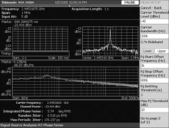
Figure 10-37. The relationship between jitter settling time and phase noise offset.

A unique feature of a frequency mask trigger is the ability to trigger on transient signals and capture a contiguous sequence of spectral data. Moreover, complex triggering provides the means to time-correlated views and markers that show the relationship between a jitter settling period and phase noise offset, as shown in Figure 10-37.
Conclusion
Along with the sustained growth in the military and mobile telephony industries, the technological innovation in RF has accelerated steadily. In particular, increased RF system development has occurred in the past two decades, and currently we are experiencing a period of intense activity in the RF industry. Consequently, to avoid interference, improve security, and advance communication capacity, modern military and commercial wireless networks have become complex. Current wireless systems typically employ sophisticated combinations of RF techniques, such as bursting, frequency hopping, CDMA, and adaptive modulation. Designing today's advanced RF equipment and successfully integrating it into working systems are complicated tasks. Moreover, the success of cellular technology and wireless data networks has caused the cost of basic RF components to plummet. This has enabled manufacturers outside the traditional military and communications markets to embed relatively complex RF devices into all sorts of commodity products. RF transmitters have become so pervasive that they can be found in almost any imaginable location, such as consumer electronics, medical devices, and industrial control systems. They can even be found in tracking devices implanted under the skin of livestock and pets.
Given the challenge of characterizing the behavior of today's RF devices, we set out in this chapter to help you understand how wireless parameters such as modulation and jitter are measured. Although this chapter has discussed the real-time spectrum analyzer (RTSA), it could have focused on the swept spectrum analyzer (SA) or the vector signal analyzer (VSA). Even though we have reached the end of our discussion, we still haven't decided what is the best instrument to use. This is because no single RF analyzer is ever the best solution for every RF measurement. In fact, many common measurements, such as the measurement of jitter in a new high-speed bus, can be performed with equal effectiveness using a swept SA, VSA, or RTSA. Today, however, the SI engineer is provided with RF benchtop instrumentation with built-in real-time analysis tools that would have been unheard of a decade ago. This adds significantly to the support and development of today's ubiquitous wireless environment.