4
BACKGROUND: PROBABILITY AND RANDOM VARIABLE THEORY
4.1 INTRODUCTION
The characterization of a random process requires an understanding of random variable theory, and this has its basis in probability theory. This chapter provides an overview of the key concepts from probability theory that underpin random variable theory. This is followed by an introduction to random variable theory and an overview of discrete and continuous random variables. The concept of expectation of a random variable is fundamental and a brief discussion is included. As part of this discussion, the characteristic function of a random variable is defined. Random variable theory is extended by the generalization to pairs of random variables and a vector of random variables. Associated concepts for this case include the joint probability mass and density functions, marginal distribution and density functions, conditional probability mass and density functions, and covariance and correlation functions. The chapter concludes with a discussion of Stirling’s formula and the important DeMoivre–Laplace and Poisson approximations to the binomial probability mass function. Useful references for probability and random variable theory include Grimmett and Stirzaker (1992) and Loeve (1977).
4.2 BASIC CONCEPTS: EXPERIMENTS-PROBABILITY THEORY
The following definitions are fundamental and define the basic concepts that underpin probability and random process theory.
4.2.1 Experiments and Sample Spaces
4.2.2 Events
4.2.3 Probability of an Event
The terminology P[A] is used to denote the probability of the event A.
4.2.3.1 Defining Probability of Experimental Outcomes
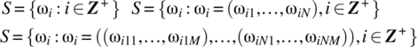
By definition, S is the set of possible experimental outcomes defined by an experiment, and each experimental outcome has a defined probability. The following two definitions are fundamental to the analysis related to random variables and apply, respectively, to the cases where the sample space comprises a countable and an uncountable number of outcomes.
4.2.3.2 Notation
The probability operator is defined on subsets of the sample space S. For the case of a countable number of outcomes, the sample space can be defined as
and P[{ω1}], P[{ω2}], etc. are well defined. For notational convenience, it is usual to write P[ω1] rather than P[{ω1}].
4.2.4 Conditional Probability
Consider an experiment that is repeated N times and performed under conditions denoted hypothesis H. Assume:
- Event A occurs NA times.
- Event B occurs NB times.
- Event
 occurs NAB times.
The relative frequency of the event ![]() is NAB/N and can be written as
is NAB/N and can be written as
As ![]() and with convergent ratios, it is reasonable to infer and define
and with convergent ratios, it is reasonable to infer and define
where P[A/(B and H)] is the probability of A assuming conditions, as specified by B and H, have occurred. As the conditions specified by H are common to all probabilities, it is usual to omit them and to write
It is common to use the notation P[AB] for ![]() .
.
4.2.4.1 Theorem of Total Probability
4.2.4.2 Bayes’ Theorem
Bayes’ theorem finds widespread application.
4.2.5 Independent Events
It is common for experiments to comprise of unrelated stages or parts. Such stages, or parts, are independent and result in independence being an outcome of the structure of the experiment. For example, consider an experiment of throwing a dice twice. The outcome of the second throw is independent of the outcome of the first throw.
Alternatively, consider a two-part experiment where the outcomes of the second part are independent of the first part. If A denotes an event based solely on the first part, and B denotes an event based solely on the second part, then
Thus, knowing that A has occurred in the first part of the experiment does not affect the probability of the event B occurring in the second part of the experiment. Similarly, ![]() . The conditional probability result
. The conditional probability result
then implies
4.2.5.1 Generalization
4.2.5.2 Independence of Elementary Events
Because of its importance, the following is stated as being axiomatic.
4.2.6 Countable and Uncountable Sample Spaces
The nature of the experiment determines the nature of the sample space. The following distinctions readily arise:
- Discrete and finite sample space:
(4.25)

- Discrete and infinite, but countable, sample space:
(4.26)

- Continuous and uncountable sample space: A continuous sample space arises when the possible outcomes from an experiment are uncountable and form a continuum. For example,
With an infinite number of outcomes, the probability of an individual point outcome (an outcome consistent with a set with zero measure) is zero. Finite probabilities are associated with intervals or collections of outcomes with nonzero length or measure. For example,
4.3 THE RANDOM VARIABLE
The outcome of an experiment, in general, is not a number and, for example, the sample space could consist of the outcomes ![]() . For such cases, it is useful to associate a number with each outcome, for example,
. For such cases, it is useful to associate a number with each outcome, for example, ![]() ,
, ![]() , and such an association defines a random variable.
, and such an association defines a random variable.
4.3.1 Notes
For the specific case where the random variable associates a distinct value X(ω) with each outcome ω in the sample space, the probability of the outcome X(ω) equals the probability of the outcome ω. This case is illustrated in Figure 4.2. Mathematically,
Figure 4.2 Illustration of the mapping associated with a random variable for the case where each experimental outcome is associated with a distinct real number.
In general, a random variable X assigns the same number to two or more experimental outcomes as illustrated in Figure 4.3. For the situation illustrated in Figure 4.3, it is the case that

Figure 4.3 Illustration of the mapping associated with a random variable for the general case where two experimental outcomes map to the same number.
It is clear that the probability of occurrence of a specific outcome for a random variable is dependent on the probability mass function, pΩ, or probability density function, fΩ, associated with the experimental outcomes.
4.3.2 Sample Spaces for Random Variables
Consider a random variable X:
For the case of a 1 : 1 structural mapping between experimental outcomes and numerical values of the associated random variable, the sample spaces, as detailed in Table 4.1, are indicative of those that arise.
Table 4.1 Forms for the sample space of a random variable
| S | Sample space SX |
| {ω1, ω2, …} | {X(ω1), X(ω2), …} |
 |
 |
 |
 |
4.3.3 Random Variable Based on Experimental Outcomes
For the case where the experimental outcomes are numerical values, a random variable ![]() can be defined based directly on the distinct experimental outcomes according to
can be defined based directly on the distinct experimental outcomes according to ![]() . For this case, the sample space SX is
. For this case, the sample space SX is
and similarly for cases where the experiment yields a vector or matrix of numerical values for each trial.
For this case, the probability mass function, or density function, of the random variable X is identical to that of the probability mass function, pΩ, or the probability density function, fΩ, associated with the experiment.
4.4 DISCRETE AND CONTINUOUS RANDOM VARIABLES
Random variables can be classified as being discrete, continuous, or a mixture of continuous and discrete. The former two types are the most common and dominate random variable theory.
4.4.1 Discrete Random Variables
4.4.1.1 Properties of Probability Mass Function
For the case where the random variable X defines the numbers {x1, …, xi, …}, the following properties hold:

4.4.2 Continuous Random Variables
4.4.2.1 Frequency Interpretation of PDF
If, in n trials of an experiment, the number of outcomes of a random variable X that fall in the interval ![]() equals nx, then
equals nx, then ![]() for n suitably large.
for n suitably large.
4.4.3 Cumulative Distribution Function
The cumulative distribution function specifies the probability that a random variable takes on a value in the interval ![]() .
.
4.4.3.1 Properties of Cumulative Distribution Function
The following properties hold for the cumulative distribution function:
 .
. .
. .
.- FX is a monotonically increasing function, that is,
For the continuous random variable case, FX is a continuous function (this follows from the assumption that fX has at most a finite number of discontinuities and is not impulsive for any values in its domain) and

The latter result holds at all points where FX is differentiable.
4.5 STANDARD RANDOM VARIABLES
The number of commonly used random variables is large. The discrete uniform, the Bernoulli, the Binomial, the Poisson, and the geometric are common discrete random variables. Common continuous random variables include the uniform, the Gaussian, the exponential, and the Rayleigh. The random variables that are used in subsequent sections, and chapters, are detailed in the reference section at the end of the book.
4.6 FUNCTIONS OF A RANDOM VARIABLE
A random variable X associates a number with each experimental outcome ω of an experiment, and the values X takes on define the sample space, SX, for the random variable. If there is a function, g, which maps each number in the sample space of the random variable X to a new subset of the real line, denoted SY, then a new random variable Y has been defined according to ![]() . These mappings are illustrated in Figure 4.5.
. These mappings are illustrated in Figure 4.5.
Figure 4.5 Illustration of mappings associated with a random variable that is a function of another random variable.
Consistent with the illustration in Figure 4.5, the random variable Y could have been defined directly on the set S of experimental outcomes. However, in many instances, the outcomes of a random variable, X, are observed, and then algebraic operations on the outcomes are undertaken consistent with a mapping as defined by a function g. Accordingly, it is natural to consider functions of a random variable.
4.7 EXPECTATION
The expectation operator allows the precise definition of various statistical properties of a random variable including the mean and variance.
4.7.1 Mean, Variance, and Moments of a Random Variable
The mean and variance are first-order measures of the nature of a random variable.
4.7.1.1 Notation
To simplify notation in the aforementioned definitions, the limits of ![]() to
to ![]() are often used for the summation, while the limits of
are often used for the summation, while the limits of ![]() and
and ![]() are often used for the integral.
are often used for the integral.
4.7.2 Expectation of a Function of a Random Variable
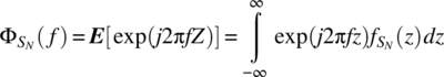
4.7.3 Characteristic Function
The characteristic function of a random variable facilitates analysis, for example, when determining the probability density function of a summation of identical random variables.
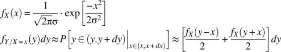
4.7.3.1 Characteristic Function of a Gaussian PDF
4.7.3.2 Characteristic Function after Linear Transformation
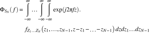
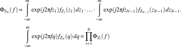
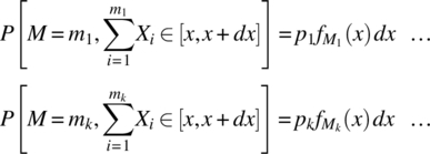
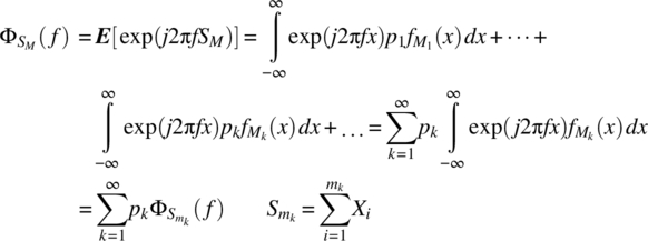
4.7.3.3 Characteristic Function of a Sum of Random Variables
4.7.3.4 PDF of a Random Sum of Gaussian Random Variables
Consider the random sum of Gaussian random variables defined according to

where M is a discrete random variable taking on the positive values m1, m2, …, with probabilities p1, p2, …, X1, X2, … is a sequence of independent Gaussian random variables and the probability density function of Xi is

4.7.3.5 PDF of a Sum of Gaussian Random Variables
The important result, which is a special case of the general result stated in Theorem 4.11, then follows.
4.7.3.6 Example
Consider the random sum of independent Gaussian random variables

where ![]() ,
, ![]() ,
, ![]() ,
, ![]() ,
, ![]() ,
, ![]() ,
, ![]() , and
, and ![]() . Consistent with Theorem 4.10, the probability density function is
. Consistent with Theorem 4.10, the probability density function is

where ![]() ,
, ![]() ,
, ![]() , and
, and ![]() . This probability density function is shown in Figure 4.6.
. This probability density function is shown in Figure 4.6.
Figure 4.6 Probability density function of a random sum of two independent random variables as specified in the text.
4.8 GENERATION OF DATA CONSISTENT WITH DEFINED PDF
Modern mathematical software packages can generate random data consistent with many standard distributions. For non-standard distributions, a method is required to generate data consistent with a defined probability density function. The usual starting point is to generate a number, uo, at random from the interval [0,1].
4.8.1 Example
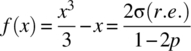
Consider a random variable with a probability density function, and a cumulative distribution function, defined according to

The transformation required is
4.9 VECTOR RANDOM VARIABLES
The experiments, whether real or hypothesized, that underpin random phenomena lead to a variety of sample spaces S:
The ith trial of an experiment will result, depending on the nature of the random phenomenon being modelled, in a single outcome ωi, a vector of outcomes ![]() , a matrix of outcomes
, a matrix of outcomes ![]() , etc. A vector of outcomes
, etc. A vector of outcomes ![]() may arise from N repeated trials of a subexperiment; a matrix of outcomes
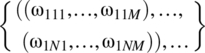
may arise from N repeated trials of a subexperiment; a matrix of outcomes ![]() may arise from N trials of a subexperiment where each subexperiment is a result of M sub-subexperiments. The following are typical forms for sample spaces:
may arise from N trials of a subexperiment where each subexperiment is a result of M sub-subexperiments. The following are typical forms for sample spaces:
When a number xi, a vector of numbers ![]() , or a matrix of numbers
, or a matrix of numbers ![]() , as appropriate, is associated with each experimental outcome, a random variable
, as appropriate, is associated with each experimental outcome, a random variable ![]() with
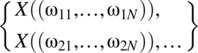
with ![]() is defined in the usual manner. The corresponding sample spaces of the random variables are
is defined in the usual manner. The corresponding sample spaces of the random variables are

4.9.1 Random Variable Defined Based on Experimental Outcomes
For the case where the experimental outcomes are numerical values, a random variable ![]() can be defined based directly on the experimental outcomes according to
can be defined based directly on the experimental outcomes according to ![]() . For this case, and with the notation
. For this case, and with the notation ![]() , the sample space SX is
, the sample space SX is ![]() . For such a case, it is usual to use the probability mass function, pΩ, or the probability density function, fΩ, of the experimental outcomes and not the corresponding function, pX or fX, of the random variable X.
. For such a case, it is usual to use the probability mass function, pΩ, or the probability density function, fΩ, of the experimental outcomes and not the corresponding function, pX or fX, of the random variable X.
4.9.2 Vector Random Variables
Consider a random variable ![]() ,
, ![]() , where SX comprises of vectors in N dimensional space consistent with
, where SX comprises of vectors in N dimensional space consistent with ![]() . For this case, the random variable can be interpreted as a vector random variable.
. For this case, the random variable can be interpreted as a vector random variable.
4.9.3 Sample Space for Vector Random Variable
Often, the values defined by a vector random variable are utilized directly, and the experiment and sample space for the random phenomena underpinning the vector random variable are left implicit. For this case, the sample space SX of the random vector is defined directly and in the following manner:
The probability ![]() associated with a specific outcome xi is usually clear.
associated with a specific outcome xi is usually clear.
4.10 PAIRS OF RANDOM VARIABLES
To establish the properties of multiple random variables, the starting point is to establish the properties for the vector random variable case of two dimensions, that is, properties for the case of ![]() . Of importance is the generalization of the ways of characterizing a random variable for the one-dimensional case: the generalization of the cumulative distribution function, the probability mass function, and the probability density function.
. Of importance is the generalization of the ways of characterizing a random variable for the one-dimensional case: the generalization of the cumulative distribution function, the probability mass function, and the probability density function.
4.10.1 Notation
For notational convenience, the vector pair of random variables (X1, X2) is written as (X, Y), and the notation ![]() is used.
is used.
The sample space for ![]() has the following general forms:
has the following general forms:

where the set RXY consists of a countable and an uncountable number of ordered pairs for, respectively, the discrete and continuous random variable cases.
4.10.2 Joint Cumulative Distribution Function (Joint CDF)
Consider a pair of random variables ![]() defined on a sample space S. The generalization of the cumulative distribution function for the one-dimensional case is the joint cumulative distribution function.
defined on a sample space S. The generalization of the cumulative distribution function for the one-dimensional case is the joint cumulative distribution function.
4.10.2.1 Properties of Cumulative Distribution Function
The cumulative distribution function has the following properties:
 .
.

- If
 and
and  , then
 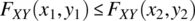 .
.  and
and 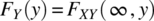 .
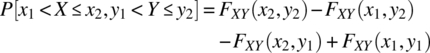
.- For the case of
 and
and  :
:
4.10.3 Joint Probability Mass Function
4.10.4 Marginal Probability Mass Function
For the joint random variable case, the individual probability mass functions are still of interest, and it is useful to be able to determine these from the joint probability mass function.
4.10.5 Joint Probability Density Function
For the case of two continuous random variables (X, Y) and consistent with the one-dimensional case, the probability of a precise value, ![]() and
and ![]() , equals zero for all values of x and y. Nonzero probabilities are only associated with intervals or sets. The joint probability density function of two continuous random variables (X, Y) can be defined in an analogous manner to the one-dimensional case.
, equals zero for all values of x and y. Nonzero probabilities are only associated with intervals or sets. The joint probability density function of two continuous random variables (X, Y) can be defined in an analogous manner to the one-dimensional case.
4.10.5.1 Relationship between PDF and CDF
If X and Y are continuous random variables with a joint probability density function, fXY, and a differentiable joint cumulative distribution function FXY, then

4.10.5.2 Properties of Joint Probability Density Function
The following properties hold for the joint probability density function:

For any subset ![]() , it is the case that
, it is the case that

4.10.6 Marginal Distribution and Density Functions
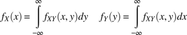
Consider a pair of continuous random variables (X, Y). The marginal cumulative distribution function, FX and FY, can be determined from the joint cumulative distribution function according to
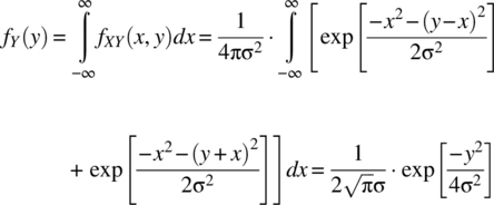
The marginal probability density function, fX and fY, can be determined from the joint probability density function according to
4.10.7 Linearity of Expectation Operator
The definition of the joint and marginal probability mass function, and the joint and marginal probability density function, allows the important linearity property of the expectation operator to be proved.
4.10.8 Conditional Mass and Density Functions
In general, the random variable ![]() where
where
is such that the random variables X and Y are not independent, that is, the occurrence of ![]() contains information about the occurrence, or non-occurrence, of
contains information about the occurrence, or non-occurrence, of ![]() and vice versa.
and vice versa.
Consider a communication channel where one trial of an experiment is to send one bit of information, denoted x, and to recover this information, denoted y, at a receiver. The outcome of the trial is the ordered pair (x, y) where ![]() for binary data communication. For a good communication channel, it is expected that
for binary data communication. For a good communication channel, it is expected that ![]() is consistent with
is consistent with ![]() and that
and that ![]() is consistent with
is consistent with ![]() , that is, reliable communication is consistent with the output data containing information about the sent, or input, data.
, that is, reliable communication is consistent with the output data containing information about the sent, or input, data.
Characterization of the dependence between two random variables is important and conditional probability mass functions, and conditional probability density functions, are widely used. Understanding these functions is facilitated by a discussion of conditioning.
4.10.8.1 Case 1: Conditioning on Subsets of Joint Sample Space
Consider ![]() , where the sample space of Z is defined by Equation 4.109, and consider events that lead to the subsets
, where the sample space of Z is defined by Equation 4.109, and consider events that lead to the subsets ![]() . It follows from the conditional probability result
. It follows from the conditional probability result ![]() , that
, that
The following notation is used:
4.10.8.2 Example
Consider the case of a random variable ![]() ,
, ![]() , which defines the sample space
, which defines the sample space
and where the probabilities of the outcomes are defined in Figure 4.9.

Figure 4.9 Probability of outcomes of the defined random variable Z.
Consider the case of ![]() ,
, ![]() , and
, and ![]() and the goal of determining PZ[A1/B] and PZ[A2/B]. First,
and the goal of determining PZ[A1/B] and PZ[A2/B]. First,
and, as the set consists of elementary events, the probability of B is

It then follows from Equation 4.110 that
4.10.8.3 Case 2: Conditioning on Subsets of Individual Sample Spaces
Consider the random variable ![]() ,
, ![]() with the sample space defined by Equation 4.109. The two component random variables X and Y are mappings:
with the sample space defined by Equation 4.109. The two component random variables X and Y are mappings:
The intersection of the events ![]() ,
, ![]() defines a subset
defines a subset ![]() :
:
The probability of occurrence of the joint events ![]() is
is
From conditional probability theory,
and the following definition can be made.
4.10.8.4 Conditional Joint Probability Mass Function
For ![]() and with the sample space defined by Equation 4.109, the joint conditional probability mass function can be defined for the case where X and Y are discrete random variables.
and with the sample space defined by Equation 4.109, the joint conditional probability mass function can be defined for the case where X and Y are discrete random variables.
4.10.8.5 Joint Conditional Probability Density Function
For ![]() and with the sample space defined by Equation 4.109, the joint conditional probability density function can be defined for the case where X and Y are continuous random variables.
and with the sample space defined by Equation 4.109, the joint conditional probability density function can be defined for the case where X and Y are continuous random variables.
4.10.8.6 Example
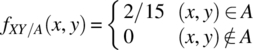
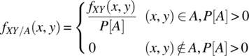
Consider the determination of the conditional joint probability density function, fXY/A, for the case of ![]() :
:
where fXY is defined according to

First, Figure 4.10 illustrates the possible outcomes of the random variable Z and the outcomes consistent with the event A. Second, the probability of the event A can be determined from the joint probability mass function:
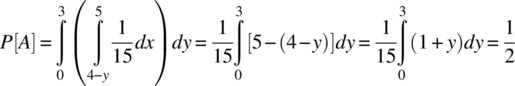
Figure 4.10 Possible outcomes of the random variable Z and the outcomes consistent with the set A.
Finally, using the result stated in Theorem 4.15, the required result follows:
4.10.8.7 Conditioning Based on Elementary Outcomes of One RV
The following general results have been established: first, for discrete random variables,

Second, for continuous random variables,
A specific subcase of these results, that of conditioning on a single outcome of one of the random variables, is widely used and of importance. The following definitions clarify notation.
4.10.8.8 Independent Case
4.11 COVARIANCE AND CORRELATION
The covariance function applies to two random variables and is a generalization of the variance function for a single random variable. A related function is the correlation function.
4.11.1 Understanding Covariance
Consider two subexperiments with countable samples spaces
which underpin an experiment with a sample space S:
The probability of individual outcomes is specified according to
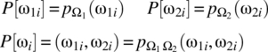
Consider the case where a random variable ![]() is defined on S according to
is defined on S according to ![]() where
where ![]() and
and ![]() define random variables on the two subexperiments in a manner such that distinct outcomes lead to distinct values for the random variables. Notation for the outcomes of the random variables is detailed in Table 4.2.
define random variables on the two subexperiments in a manner such that distinct outcomes lead to distinct values for the random variables. Notation for the outcomes of the random variables is detailed in Table 4.2.
Table 4.2 Outcomes of the random variables Z, X, and Y
| ω | Z(ω) | X(ω) | Y(ω) |
| ω1 | |||
| ω2 | |||
| ω3 | |||
| … |
The joint probability of (xi, yj) is ![]() , and for the case where X is independent of Y, it is the case that
, and for the case where X is independent of Y, it is the case that ![]() .
.
The following measures can be proposed for the dependence of the random variables X and Y for the specific case of the outcome (xi, yj):

Consider the first measure. When this measure is weighted by the values of the random variables according to
and summed over all possible outcomes, a mean measure for the dependence of the random variables X and Y is obtained according to
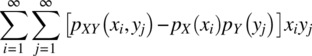
This measure is the covariance function of the two random variables X and Y as the following analysis shows:
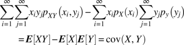
The covariance function utilizes the simplest measure for the dependence between two random variables.
4.11.2 Uncorrelatedness
The concept of uncorrelatedness for two random variables arises from the definition of the covariance.
4.11.2.1 Independence Implies Uncorrelatedness
4.11.2.2 Example: Uncorrelated and Dependent Pair of Random Variables
Consider the case of a random variable ![]() ,
, ![]() with outcomes of the form
with outcomes of the form

and with
It then follows that


It then follows that ![]() , which implies dependence between X and Y. The covariance between X and Y is zero as
, which implies dependence between X and Y. The covariance between X and Y is zero as

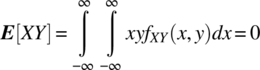
Thus, the random variables are uncorrelated but dependent. The joint probability density function is shown in Figure 4.12 for the case of ![]() .
.

Figure 4.12 Graph of the joint probability density function for the case of σ2 = 1.
4.11.3 The Correlation Coefficient
The correlation coefficient is widely used as it gives a normalized measure of the correlation between two random variables.
4.12 SUMS OF RANDOM VARIABLES
Consider the random variable Z that is defined as the weighted summation of N random variables X1, …, XN according to
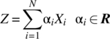
The following important results hold.
4.12.1 Sum of Gaussian Random Variables
The probability density function for a sum of independent Gaussian random variables has been detailed in Theorem 4.11.
4.12.2 Difficulty in Determining the PDF of a Sum of Random Variables
In general and consistent with the ![]() -fold integral expression specified in Equation 4.181, determining the probability density function of a sum of random variables is difficult.
-fold integral expression specified in Equation 4.181, determining the probability density function of a sum of random variables is difficult.
4.13 JOINTLY GAUSSIAN RANDOM VARIABLES
The number of useful joint probability mass functions and joint probability density functions is large. The most widely used joint probability density function is the bivariate Gaussian.
4.14 STIRLING’S FORMULA AND APPROXIMATIONS TO BINOMIAL
The outcomes of complex phenomena, in many instances, can be modelled based on the outcomes of repetitions of a simple experiment. The simplest experiment is the Bernoulli experiment with two outcomes: success or failure. The probability of a specific outcome arising from a large number of repetitions of such an experiment is specified by the binomial probability mass function. This probability mass function is in terms of factorials and powers and computational complexity is reduced if suitable approximations can be defined. The two important approximations are the DeMoivre–Laplace approximation and the Poisson approximation. Both approximations are based on Stirling’s formula, which states an approximation to a factorial number.
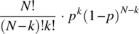
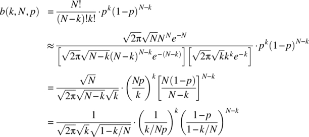
4.14.1 Binomial Probability Mass Function
4.14.2 Stirling’s Formula
Stirling’s formula (Stirling, 1730; Feller, 1957, p. 50f; Parzen, 1960, p. 242) provides an accurate approximation to the factorial of a number.
4.14.3 DeMoivre–Laplace Theorem
The first important approximation to the binomial probability mass function is the DeMoivre–Laplace approximation (Feller, 1945; Feller, 1957, p. 168f; Papoulis and Pillai, 2002, p. 105f).
4.14.3.1 Notes
For the case of ![]() , the relative error is usually small. For a given N and μ and a set bound on the relative error, a nonlinear root solving algorithm can be used on Equation 4.191 to solve for the range of k for which the DeMoivre–Laplace approximation is valid.
, the relative error is usually small. For a given N and μ and a set bound on the relative error, a nonlinear root solving algorithm can be used on Equation 4.191 to solve for the range of k for which the DeMoivre–Laplace approximation is valid.
4.14.3.2 Example
The binomial probability mass function, along with the relative error and the approximation to the relative error as given by Equation 4.191, is shown in Figure 4.15 for the case of ![]() and
and ![]() . The DeMoivre–Laplace approximation is valid, with a relative error less than 0.1, for
. The DeMoivre–Laplace approximation is valid, with a relative error less than 0.1, for ![]() assuming the relative error expression specified in Equation 4.191. The approximate range for k, as given by Equation 4.192, is
assuming the relative error expression specified in Equation 4.191. The approximate range for k, as given by Equation 4.192, is ![]() , which is slightly conservative. This arises as
, which is slightly conservative. This arises as 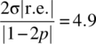 .
.

Figure 4.15 Relative error (dots) and relative error approximation (line) for the DeMoivre–Laplace approximation to the binomial probability mass function for the case of N = 100 and p = 0.4.
4.14.3.3 Generalization
The following theorem specifies a useful extension of the DeMoivre–Laplace theorem.
4.14.4 Poisson Approximation to Binomial
For the case when ![]() and
and ![]() , the Poisson approximation to the binomial probability mass function is appropriate (Feller, 1957, p. 142f).
, the Poisson approximation to the binomial probability mass function is appropriate (Feller, 1957, p. 142f).
4.14.4.1 Example
The binomial probability mass function, along with the relative error and relative error approximation as given by the two expressions in Equation 4.199, are shown in Figure 4.16 for the case of ![]() and
and ![]() . The Poisson approximation is valid as
. The Poisson approximation is valid as ![]() ,
, ![]() ,
, ![]() , and the region of validity, as given by
, and the region of validity, as given by ![]() , is
, is ![]() .
.
Figure 4.16 Binomial probability mass function for the case of N = 100 and p = 0.015 and the relative error (dots), and relative error approximation (line), in the Poisson approximation to this probability mass function.
4.15 PROBLEMS
- 4.1 From the three axioms defining the probability measure, show that:
 .
. - 4.2 Show that the probability operator is a valid measure.
- 4.3 If the events A and B are independent, then show that the events A and BC are independent.
- 4.4 From conditional probability theory, and the Theorem of Total Probability, proves Bayes’ theorem:
(4.200)
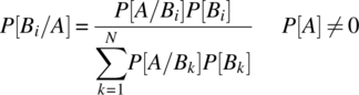
assuming the set of events {B1, …, BN} is a partition of the sample space.
- 4.5 Binary communication from a transmitter to a receiver is widely used. The sample space for communication of one bit of information in such a communication system is
(4.201)

where the first element in the ordered pair represents the sent information and the second element represents the received information.
- Specify an expression for the probability of error in the transmission of one bit assuming the following definitions:
(4.202)

- Use Bayes’ theorem to determine an expression for P[1 sent/1 received], that is, the probability of a logic one was sent given a logic one was received.
- Determine P[1 sent/1 received], and the probability of error, for the case of
 and
and  .
.
- Specify an expression for the probability of error in the transmission of one bit assuming the following definitions:
- 4.6 Specify the sample space of the experiment where each trial consists of:
- Choosing a number at random from the interval
 .
. - Choosing a second number, at random, between the first one and one.
- Choosing a number at random from the interval
- 4.7 A trial of an experiment comprises of the running of N independent subexperiments. Each subexperiment yields outcomes from the set {A, B, C}. Specify the sample space for this experiment.
- 4.8 A degenerate random variable is defined on an experiment with only one outcome, that is,
 . If a degenerate random variable is defined according to
  , then specify, and graph, the probability mass function, and cumulative distribution function, for this random variable.
 - 4.9 An indicator random variable is defined according to
(4.203)
where A is a subset of S. Define, and graph, the probability mass function, and the cumulative distribution function, of X.
- 4.10 Consider an experiment based on a very large number of independent subexperiments with outcomes of success or failure. The probability of success in one of the subexperiments is p. Define the random variable X as the number of trials of the subexperiment before the first success. This random variable is called the geometric random variable.
- Specify the probability mass function for X.
- Graph the probability mass function for the case of
 .
. - Show that
(4.204)
This result states a memoryless property: if there have been no successes up until the koth subexperiment, then the probability of the first success occurring after a further k1 subexperiments is independent of ko.
- 4.11 Consider a fixed positive integer r and an experiment based on a very large number of independent subexperiments with outcomes of success or failure. The probability of success in one of the subexperiments is p. Define the random variable X as the number of failures prior to the rth success (the waiting time for the rth success).
- Specify the probability mass function for X.
- Graph the probability mass function for the case of
 and
and  .
. - Graph the probability mass function for the case of
 and
and  .
.
- 4.12 Photons are incident on a photodetector at random times and such that
(4.205)
where λ is the mean arrival rate. The probability mass function is Poisson with a parameter λT. By considering an infinite number of such detectors, and the experiment of choosing one photodetector at random, an experimental sample space can be defined based on the photon arrival times.
- For a fixed interval [0, T], a random variable X is defined as the number of photons that have arrived. Graph the probability mass function of this random variable for the case of
 and
and  .
. - A random variable Y is defined as the time the first photon arrives. Determine the cumulative distribution function, and the probability density function, of this random variable.
- For a fixed interval [0, T], a random variable X is defined as the number of photons that have arrived. Graph the probability mass function of this random variable for the case of
- 4.13 A particle is emitted from a source and impacts, at random, on a hemisphere of radius r. The point of impact is defined by
 where
where  is the latitude and
  is the longitude. If the emission of one particle from the source is considered as one trial of an experiment, then the set of possible points of impact define an experimental sample space. A random variable is defined on this sample space according to
  . Determine the cumulative distribution function, and the probability density function, of X.
 - 4.14 Consider an experiment that yields points on the plane and the experimental sample space
 . The points are such that two random variables X, Y, defined according to
  and
and  , are independent and have zero mean Gaussian density functions, that is,
(4.206)
, are independent and have zero mean Gaussian density functions, that is,
(4.206)
A new random variable, Z, is defined according to
(4.207)
which is the magnitude of the vector defined by each point. Note that
(4.208)
where
 . Determine the probability density function, and cumulative distribution function, of Z. This probability density function finds widespread application in communications.
 - 4.15 Find the expected value, the expected squared value, and the variance of a random variable X that has a Poisson probability mass function with a parameter λ:
(4.209)
- 4.16 A random variable X with a Rayleigh distribution has a probability density function given by
(4.210)
Determine the mean and variance of X.
- 4.17 A random variable Y is defined on a continuous random variable X according to
(4.211)

Determine the probability density function of Y in terms of the probability density function of X.
- 4.18 A discrete random variable Y is defined on a continuous random variable X according to
 . Determine the probability mass function of X.
 - 4.19 Determine the characteristic function of a random variable that has a Poisson distribution with a parameter λ.
- 4.20 A random variable Z is defined as the sum of two independent random variables X1 and X2 where X1 has a Poisson distribution with parameter λ1 and X2 has a Poisson distribution with parameter λ2.
- Determine the characteristic function of Z.
- Determine the probability mass function of Z.
- 4.21 Consider the experiment consistent with a ternary communication signalling protocol, which is defined as follows:
- A number is chosen, at random, from the set
 .
. - A second number is chosen from the set
 subject to the constraint that if the number is nonzero, then it cannot be the same as the previous number.
 - A third number is chosen in a manner consistent with the second number and this procedure is repeated N times.
- Specify the set of experimental outcomes for the case of
 .
. - Specify the probability of each outcome for the case of
 assuming
  , and
, and  .
.
- Specify the set of experimental outcomes for the case of
- A number is chosen, at random, from the set
- 4.22 Consider the experiment defined as follows:
- A number is chosen at random from the set {0, 1}. A second number is chosen at random from the interval
 .
. - The procedure specified in (i) is repeated N times.
Specify the set of experimental outcomes.
- A number is chosen at random from the set {0, 1}. A second number is chosen at random from the interval
- 4.23 Consider an experiment based on throwing two die and noting the pair of numbers. An experimental outcome is denoted
 . A pair of random variables
  is defined on this experiment according to
(4.212)
is defined on this experiment according to
(4.212)
- Specify the sample space for Z.
- Specify the joint probability mass function of X and Y.
- Determine the marginal probability mass function for X.
- Determine the marginal probability mass function for Y.
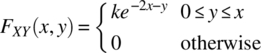
- 4.24 The joint cumulative distribution function of two continuous random variables X and Y is
(4.213)
- Determine k.
- Determine
 .
. - Determine
 .
. - Determine the joint probability density function of X and Y.
- Determine the marginal probability density functions of X and Y.
- 4.25 Two random variables have a joint probability density function
(4.214)
- Determine k.
- Determine the marginal probability density functions of X and Y.
- Are X and Y independent?
- Determine the probability of
 .
.
- 4.26 An experiment yields the following experimental sample space:
(4.215)

and the probability of occurrence of a given outcome is
 . Two random variables, and an event A, are defined on this sample space according to(4.216)
 (4.217)
Determine the conditional probability mass function pXY/A(x, y) for the case of
 and for the general case where
  .
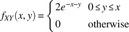
. - 4.27 The random variables X and Y have a joint probability density function
(4.218)

- Determine the constant k.
- Find the conditional probability density function fXY/A(x, y) for the case of
(4.219)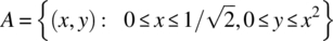
- 4.28 The joint probability density function of two random variables X and Y is
(4.220)
- Determine
 .
. - Determine
 .
.
- Determine
- 4.29 In a communication system and at a set time, a signal is detected, which has the form
(4.221)

where X and Y are independent random variables with probability density functions:
(4.222)
- Determine E[Z].
- Determine E[Z2] and the variance of Z.
- If the random variable Y represents a noise signal, specify a general condition for the recovery of the amplitude A from Z2.
- 4.30 Establish the variance of
 .
. - 4.31 If
 and
and  , where Θ is a random variable with a uniform distribution on
  , then determine the mean and variance of X and Y and the correlation coefficient ρXY.
 - 4.32 Prove the result that the probability of k successes in N independent trials of an experiment is
(4.223)
when the probability of success in an independent trial is p.
- 4.33 Determine the mean and variance of a random variable X with a binomial probability mass function.
- 4.34 If X and Y are random variables with a bivariate Gaussian joint density function, then determine the marginal density functions of X and Y.
- 4.35 Consider the DeMoivre–Laplace approximation to the binomial probability mass function for the case of
 and
and  . Graph the relative error and the approximation to the relative error as given by
(4.224)
. Graph the relative error and the approximation to the relative error as given by
(4.224)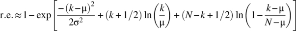
Determine the range of validity of the DeMoivre–Laplace approximation for a relative error of less than 0.1 and compare these values with the range
(4.225)
- 4.36 Check the error bound
(4.226)

for the Poisson approximation to the binomial probability mass function by considering the following values: (i)
 , (ii)
  , and (iii)
  .
. - 4.37 The probability that a voter in an election is conservative equals 0.4. Consider 1000 voters, chosen at random. Determine the probability, among the 1000 voters, that the number of conservative voters is between, and including the bounds, 370 and 395.
- 4.38 In the industrial sector of a country, the probability of a worker having an accident that requires surgery on a single working day is
 .
.
- What is the probability that a worker does not have an accident requiring surgery in his career spanning 104 working days.
- In a working year of 300 days and in a factory with 1000 workers, what is the probability of zero, one, or two accidents requiring surgery? What is the probability of one or more accidents?
APPENDIX 4.A PROOF OF THEOREM 4.6
By definition

The integral is that of a Gaussian probability density function with a mean of ![]() and a variance of σ2, and accordingly, the integral is unity. The required result of
and a variance of σ2, and accordingly, the integral is unity. The required result of
then follows. The final result arises by using the association ![]() .
.
APPENDIX 4.B PROOF OF THEOREM 4.8
By definition
From Theorem 4.23,

Interchanging the order of integration yields
A change of variable ![]() in the inner integral results in
in the inner integral results in

The assumption of independence yields the required result:
The result for a weighted sum follows from the relationship given in Theorem 4.7: if ![]() , then
, then ![]() .
.
APPENDIX 4.C PROOF OF THEOREM 4.9
Consider the disjoint outcomes of SM and their associated probabilities:
where ![]() is the probability density function of
is the probability density function of ![]() . It then follows that
. It then follows that
The assumption of independent random variables, and the result for the characteristic function of a sum of independent random variables stated in Theorem 4.8, yields the required result:

APPENDIX 4.D PROOF OF THEOREM 4.21
Consider a random variable ![]() for some constant α. Consider
for some constant α. Consider

Since ![]() , it follows that
, it follows that
and
for all values of α. With ![]() , the upper bound for the correlation coefficient results according to
, the upper bound for the correlation coefficient results according to

The lower bound for the correlation coefficient arises by choosing ![]() and proceeding in a similar manner.
and proceeding in a similar manner.
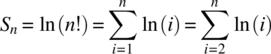
APPENDIX 4.E PROOF OF STIRLING’S FORMULA
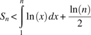
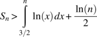
Stirling’s formula can be proved by considering upper and lower bounds on the summation
To determine an upper bound on Sn, consider the integral  and the integral approximation illustrated in Figure 4.17. Consistent with the areas defined in this figure, it follows that

Figure 4.17 Areas defined by an affine approximation to the integral ln(x) on the interval [1, n].
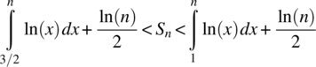
Hence, an upper bound for Sn is
To determine a lower bound for Sn, consider an affine, and tangent, approximation to ln(x) around the point ![]() as illustrated in Figure 4.18. Consistent with the tangent approximation illustrated in this Figure, it follows that
as illustrated in Figure 4.18. Consistent with the tangent approximation illustrated in this Figure, it follows that

Figure 4.18 An affine, and tangent, approximation to ln(x) around the point x = i.
As ln(x) is monotonically increasing, it follows that
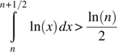
and, hence,
Combining the upper and lower bounds for Sn, as given by Equations 4.243 and 4.246, yields
Evaluation of the integrals using the result
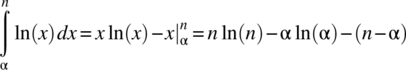
and substitution of the definition ![]() yields
yields

Hence,

As the exponential function is a monotonically increasing function, it follows that
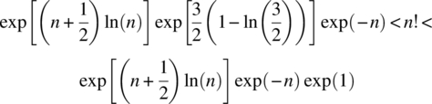
and thus,

It can be shown that the limit of the sequence ![]() is
is ![]() . It is the case that
. It is the case that ![]() equals 2.527597, 2.508718, 2.506837, respectively, for the case of
equals 2.527597, 2.508718, 2.506837, respectively, for the case of ![]() . Hence,
. Hence,

The relative error bound in the approximation ![]() is
is
APPENDIX 4.F PROOF OF THEOREM 4.27
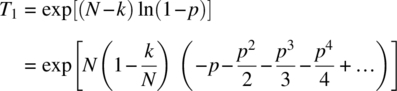
Consider the use of Stirling’s formula ![]() on the result for k successes in N trials, that is,
on the result for k successes in N trials, that is,
which is the first required result. Using the relationship ![]() yields the second required form
yields the second required form

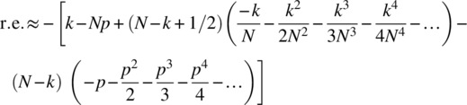
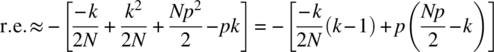
To establish the third result, define the difference between k and the mean value of k, as given by Np, as Δk, that is, ![]() . The following results then hold
. The following results then hold

Substitution of these results into Equation 4.255 yields

With the manipulations

and ![]() , it follows that
, it follows that

Consider the expression

Taking the natural logarithm yields

Consider the expansion ![]() , which can be applied provided
, which can be applied provided

Use of this expansion leads to

Expanding and collecting terms yields the following result:
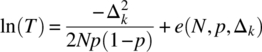
where

It then follows that

When e(N, p, Δk) « 1, the DeMoivre–Laplace approximation follows from the definitions ![]() and
and ![]() , that is,
, that is,

4.F.1 Relative Error
The relative error in the DeMoivre–Laplace approximation is
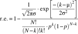
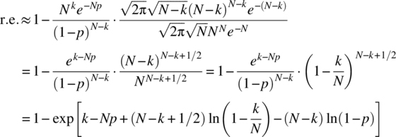
The DeMoivre–Laplace approximation is based on using Stirling’s formula, and the relative error in this approximation is small for N moderate to large. Accordingly, using Equation 4.260, a reasonable approximation to the relative error is

To obtain the last equation, the result ![]() has been used and this is the stated relative error expression.
has been used and this is the stated relative error expression.
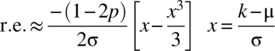
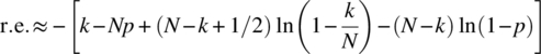
An alternative approximation to the relative error can be obtained by considering Equation 4.267:
assuming ![]() . For the case of
. For the case of ![]() and
and ![]() , a simplified relative error approximation can be obtained from Equation 4.266 according to
, a simplified relative error approximation can be obtained from Equation 4.266 according to

The first and third terms typically dominate the second term and with ![]() :
:
To determine the range of values of k, where the approximation is within a set relative error, the equation  . can be solved for x and hence k. To this end, consider the function
For the case of ![]() , the approximation
, the approximation ![]() yields a relative error of less than 10% in the solution of
yields a relative error of less than 10% in the solution of ![]() . With such an approximation, it follows that values of k in the range
. With such an approximation, it follows that values of k in the range

satisfy the relative error criterion. Hence, for a set relative error,

APPENDIX 4.G PROOF OF THEOREM 4.29
As ![]() , it follows that
, it follows that

Consider ![]() , which can be written as
, which can be written as
using the expansion ![]() . It then follows, assuming
. It then follows, assuming ![]() and
and ![]() , that
, that ![]() . With the additional assumption of
. With the additional assumption of ![]() , the required approximation follows, that is,
, the required approximation follows, that is,
The relative error in this approximation is

Stirling’s formula ![]() yields
yields
The relative error is small when the magnitude of the argument of the exponential term is much less than one such that the approximation
is valid. To determine when the relative error is small, consider the approximation noted earlier for ![]() , which yields
, which yields
Expanding out and collecting terms yields

With the existing assumptions of ![]() , the further assumptions of
, the further assumptions of ![]() and
and ![]() are required for the relative error to be small. The restrictions on k then are
are required for the relative error to be small. The restrictions on k then are
The assumption of ![]() implies that
implies that ![]() . In summary, the constraints for the validity of the Poisson approximation are
. In summary, the constraints for the validity of the Poisson approximation are ![]() . When these constraints hold, the relative error can be approximated according to
. When these constraints hold, the relative error can be approximated according to
which is the required result.