7
CHARACTERIZING RANDOM PROCESSES
7.1 INTRODUCTION
There are many ways a random process can be characterized, and the characterization is usually linked to the application or situation in which it arises and the information required. The most common ways of characterizing random processes is via the evolution with time of the probability mass/density function, an autocorrelation function, and a power spectral density function. This chapter provides an introduction to such characterization, and this is followed by associated material including correlation, the average power in a random process, stationarity, Cramer’s representation of random processes, and the state space characterization of random processes. One-dimensional random processes are assumed.
7.1.1 Notation for One-Dimensional Random Processes
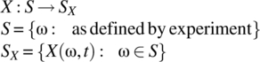
Consistent with the notation introduced in Chapter 5 and used in Chapter 6, the following notation is used for a random process X:
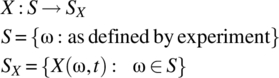
For notational convenience, a random process is written as X(Ω, t) with the interpretation
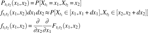
The probability of a specific experimental outcome is governed by a probability mass function or a probability density function:
In this chapter, the signals are assumed to be one-dimensional as illustrated in Figure 7.1.
Figure 7.1 Illustration of signals defined by a random process for the one-dimensional case and the values determined by the random variable defined by the random process at the time t0.
7.1.1.1 Random Variables Defined by a Random Process
For a random process that defines one-dimensional signals, the values defined by the signals of the random process, at a specific time t0, define a random variable ![]() :
:

By varying the time from t0 to t1 to t2, etc., an infinite sequence of random variables can be defined.
7.1.2 Associated Random Processes
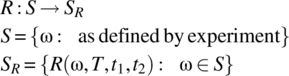
Consider a one-dimensional random process:
The following associated random processes, for example, can be defined:

Here, X1 is a random process defined by the magnitude squared of the signals arising from X. X2 is a random process, for τ fixed, defined by the autocorrelation function of the signals arising from X. X3 is a random process defined by the Fourier transform of the signals arising from X, and X4 is a random process defined by the power spectral density of the signals arising from X. Signals from X, X1, and X3 are illustrated in Figure 7.2.
Figure 7.2 Illustration of the ith signals defined by a random process X and the associated random processes X1 and X3.
7.2 TIME EVOLUTION OF PMF OR PDF
For all values of time, where the signals defined by a random process are valid, a random variable is defined that has a probability mass function, a probability density function, or outcomes that form both a countable set and an uncountable set (the mixed random variable case). The former two cases dominate the latter case, and these are considered. The probability mass function, or probability density function, changes with time to result in an evolving function. The evolution with time of the probability mass function, or probability density function, provides useful information about a random process.
For a discrete state random process, the time-evolving probability mass function is denoted pX(t)(x) and is defined according to
where, for a fixed time t, the random variable defined, consistent with the notation above, is denoted Xt.
For a continuous state random process, the time-evolving probability density function is denoted fX(t)(x) and is defined according to
for dx sufficiently small.
This evolution is illustrated in Figure 7.3 for the case of a discrete time–discrete state random process and in Figure 7.4 for the case of a continuous time–continuous state random process.
Figure 7.3 Illustration of the evolution of probability mass function for a discrete time–discrete state random process.

Figure 7.4 Illustration of the evolution of the probability density function for a continuous time–continuous state random process.
7.3 FIRST-, SECOND-, AND HIGHER-ORDER CHARACTERIZATION
As a random process, at a set time, defines a random variable, it follows that random variable theory finds widespread application in characterizing random processes. The following first-, second-, and higher-order characterizations are fundamental.
7.3.1 First-Order Characterization
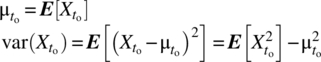
Consider a random variable ![]() defined by a random process at a fixed time to. The following parameters and functions can be defined: first, the mean and variance:
defined by a random process at a fixed time to. The following parameters and functions can be defined: first, the mean and variance:
Second, the cumulative distribution function:
Third, the probability mass function for the case where ![]() is a discrete random variable and the probability density function for the case where
is a discrete random variable and the probability density function for the case where ![]() is a continuous random variable:
is a continuous random variable:
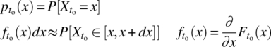
Here, dx is assumed to be sufficiently small.
7.3.2 Second-Order Characterization
Consider the two random variables ![]() and
and ![]() defined by the fixed times t1 and t2. Apart from the mean, variance, cumulative distribution function, probability mass function, or probability density function, of the individual random variables, the following functions can be defined. First, the joint cumulative distribution function:
defined by the fixed times t1 and t2. Apart from the mean, variance, cumulative distribution function, probability mass function, or probability density function, of the individual random variables, the following functions can be defined. First, the joint cumulative distribution function:
Second, the joint probability mass function for the case where ![]() and
and ![]() are discrete random variables and the joint probability density function for the case where
are discrete random variables and the joint probability density function for the case where ![]() and
and ![]() are continuous random variables:
are continuous random variables:
Here, dx1 and dx2 are assumed to be sufficiently small.
7.3.3 Nth-Order Characterization
Consider the N random variables ![]() defined by the fixed times t1, …, tN. Apart from the mean, variance, cumulative distribution function, probability mass/density function of the individual random variables or the joint cumulative distribution and joint probability mass/density function of pairs of random variables, the following functions can be defined. First, the joint cumulative distribution function of the N random variables:
defined by the fixed times t1, …, tN. Apart from the mean, variance, cumulative distribution function, probability mass/density function of the individual random variables or the joint cumulative distribution and joint probability mass/density function of pairs of random variables, the following functions can be defined. First, the joint cumulative distribution function of the N random variables:
The constraints, on a random process, defined by the joint cumulative distribution function are illustrated in Figure 7.5.

Figure 7.5 Illustration of the constraints on a random process as defined by the joint cumulative distribution function.
Second, the joint probability mass function for the case where ![]() are discrete random variables and the joint probability density function for the case where
are discrete random variables and the joint probability density function for the case where ![]() are continuous random variables, respectively, are defined according to
are continuous random variables, respectively, are defined according to
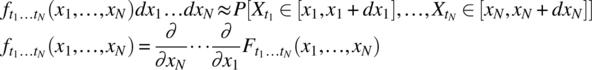
Here, dx1 … dxN are assumed to be sufficiently small.
As a random process defined on the real line defines an uncountable number of random variables, it follows that a complete specification of such a random process, in terms of a joint probability density function, is not possible.
7.3.4 Mean and Variance and Average Power
Based on a first-order characterization, the following functions give useful information about a random process X.
7.3.4.1 Instantaneous Power
The average power, as defined by Equation 7.21, is consistent with the following definition of instantaneous power.
7.3.4.2 Example
Consider a random process defined as the sum of two random processes:
The instantaneous power of X is

where ![]() for
for ![]() is the instantaneous power in Xi. Thus, uncorrelatedness implies addition of individual powers; correlation implies that the addition of individual powers does not hold.
is the instantaneous power in Xi. Thus, uncorrelatedness implies addition of individual powers; correlation implies that the addition of individual powers does not hold.
Consider the case of
where ![]() and
and ![]() . It then follows that
. It then follows that
assuming A1 and A2 are independent of Φ1 and Φ2. For the case where one or both of E[A1A2] and ![]() are zero, the instantaneous power of X equals the sum of the instantaneous powers of X1 and X2.
are zero, the instantaneous power of X equals the sum of the instantaneous powers of X1 and X2.
7.3.5 Transient, Steady-State, Periodic, and Aperiodic Random Processes
The definitions for the mean, and mean squared value, of a random process allows the following classification of random processes.
7.4 AUTOCORRELATION AND POWER SPECTRAL DENSITY
The two most widely used approaches for characterizing a random process is via an autocorrelation function and via a power spectral density function. The transition from the signal definitions for the autocorrelation function and the power spectral density function to equivalent definitions for a random process is via the expectation operator. A review of the signal definitions for these functions is useful.
7.4.1 Definitions for Individual Signals
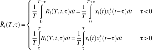
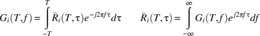
Consider a random process ![]() . Each signal in the signal sample space SX has an autocorrelation, a time-averaged autocorrelation, and a power spectral density consistent with the definitions in Chapter 3. For the ωth signal and the interval [0, T], these definitions are
. Each signal in the signal sample space SX has an autocorrelation, a time-averaged autocorrelation, and a power spectral density consistent with the definitions in Chapter 3. For the ωth signal and the interval [0, T], these definitions are

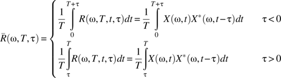
where X(ω, T, f) is the Fourier transform of X(ω, t) evaluated over the interval [0, T].
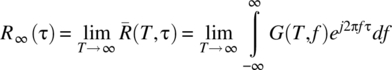
The time-averaged autocorrelation–power spectral density function relationships are
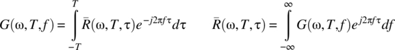
Sufficient conditions for the existence of the individual power spectral density and time-averaged autocorrelation functions have been detailed in Chapter 3, and the relationships between G(ω, T, f) and ![]() are valid when
are valid when ![]() and X(ω, t) is piecewise differentiable on [0, T].
and X(ω, t) is piecewise differentiable on [0, T].
7.4.1.1 Associated Autocorrelation and PSD Random Processes
The collection of autocorrelation and power spectral density functions defined by a random process X define the following associated random processes:
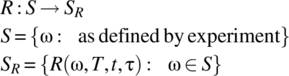
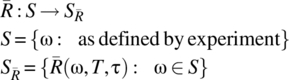

Convenient notation for these associated random processes are R(Ω, T, t1, t2), R(Ω, T, t, τ), ![]() , and G(Ω, T, f).
, and G(Ω, T, f).
7.4.2 Definitions for Autocorrelation and PSD
The following definitions can be made by considering the expectation over the appropriate signal sample space.
7.4.3 Simplified Notation: Countable Signal Sample Space Case
For the case of a countable space of experimental outcomes
where the probability of the ith outcome is ![]() , the notation for a random process X, as follows, is useful:
, the notation for a random process X, as follows, is useful:

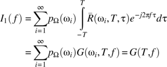
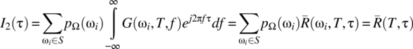
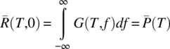
The following simplified notation holds for the autocorrelation and power spectral density functions: for the ith signal,
and the time-averaged autocorrelation–power spectral density function relationships are
7.4.3.1 Definitions
The following definitions for functions that characterize a random process can then be made.
7.4.4 Notation: Vector Case
In many cases, the experiment underpinning the random process ![]() defines N random variables
defines N random variables ![]() where
where

The first definition is for the discrete random variable case; the second definition is for the continuous random variable case. For the continuous random variable case, the following definitions apply.
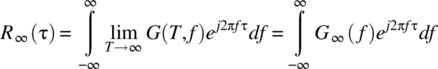
7.4.5 Infinite Interval Case
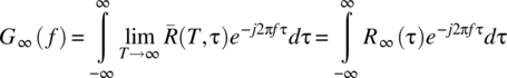
The time-averaged autocorrelation function, and the power spectral density function, of individual signals from a random process can be defined on the infinite interval ![]() as a limit according to
as a limit according to
The expectation over the ensemble of signals leads to the following definitions.
7.4.6 Existence: Finite Interval
7.4.7 Existence: Infinite Interval
7.4.7.1 Power Spectral Density: Infinite Interval
7.4.8 Power Spectral Density–Autocorrelation Relationship
7.4.8.1 Finite Interval
The relationship between the power spectral density function and the time-averaged autocorrelation function is via the Fourier transform according to the following theorem.
7.4.8.2 Infinite Interval Case: Wiener–Khintchine Relationships
Additional restrictions are required for the power spectral density–autocorrelation function relationships to hold on the infinite interval.
7.4.8.3 Impulsive Case: Formal Definition of Wiener–Khintchine
When the signals defined by a random process contain periodic components, the power spectral density G(T, f) becomes impulsive, at specific values of f, as ![]() , and it is not possible to interchange the order of limit and integration in the following equation:
, and it is not possible to interchange the order of limit and integration in the following equation:
For this case, a spectral distribution function is defined.
7.4.9 Notes on Spectral Characterization
The most widely used approach for characterizing random phenomena in engineering and science is through the use of the power spectral density function. Further, it is common to characterize stationary random processes according to the nature of their spectrum and without reference to the underlying time domain signals or underlying experiments. Examples include white noise with a power spectral density specified as
or 1/f noise random processes with a power spectral density specified as
Both definitions, however, are problematic as they imply infinite power random processes.
7.5 CORRELATION
For notational convenience, the argument T is dropped from the autocorrelation functions and a subscript of XX for a random process X is added, that is, R(T, t1, t2) is written as RXX(t1, t2).
7.5.1 Correlation Coefficient
A correlation coefficient can be defined, as in Section 4.11.3, for any two random variables. Accordingly, the following definition can be made.
7.5.1.1 Correlation Time
It can be useful to have a measure of the time over which a random process is correlated. One approach is to determine the time τ for the correlation coefficient to change from unity at the times (t, t) to a predefined level at the times ![]() .
.
7.5.2 Expected Change in a Specified Interval
Another useful characteristic of a random process is its expected change over a set interval.
7.5.2.1 Application
For a set resolution in amplitude Δx and for a given random process, it is possible to find the maximum time resolution Δt such that
This information can be used to set the sampling time required to ascertain, for example, the first passage time or maximum level, consistent with an amplitude resolution of Δx.
7.6 NOTES ON AVERAGE POWER AND AVERAGE ENERGY
When an orthonormal basis set is used for signal decomposition, the average power, or average energy, in a random process is given by the weighted average of the powers, or energies, in the individual component signals.
7.6.1 Power and Energy: Uncorrelated Coefficients
Orthonormality guarantees that the average power, or average energy, on an interval is the summation of the powers in the individual signal components. It is of interest if this result also holds for the case where the waveforms in a decomposition are not necessarily orthonormal or orthogonal.
7.6.2 Sufficient Conditions for Uncorrelated Coefficients
Consider a sinusoidal basis set ![]() for the interval [0, T]. Assume a random process
for the interval [0, T]. Assume a random process ![]() which is such that each defined signal has a Fourier series decomposition on the interval [0, T]:
which is such that each defined signal has a Fourier series decomposition on the interval [0, T]:
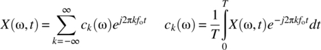
The kth coefficients define a random variable Ck with outcomes ![]() . The uncorrelatedness of the coefficients Ci and Ck for
. The uncorrelatedness of the coefficients Ci and Ck for ![]() , that is,
, that is, ![]() , as
, as ![]() depends on the autocorrelation function,
depends on the autocorrelation function, ![]() , and on the interval [0, T].
, and on the interval [0, T].
7.6.2.1 Notes
For t fixed the region of integration for the integral in Equation 7.102 is illustrated in Figure 7.6.
Figure 7.6 Region where the autocorrelation function RXX (t + τ, t) is nonzero assuming the interval [0,T].
The random variables Ci and Ck, in general, vary with T. However, the result of the convergence of ![]() to zero,
to zero, ![]() , is guaranteed when the autocorrelation function is integrable on the infinite interval such that Equation 7.102 holds.
, is guaranteed when the autocorrelation function is integrable on the infinite interval such that Equation 7.102 holds.
Writing the autocorrelation function in terms of the correlation function (see Eq. 7.83) according to
it follows that sufficient conditions for Equation 7.102 to hold are as follows: ![]() for all t, boundedness of the variance, that is,
for all t, boundedness of the variance, that is,
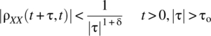
and for the random process to be increasingly uncorrelated at the times ![]() and t, as
and t, as ![]() , consistent with the existence of constants
, consistent with the existence of constants ![]() , τo independent of t, such that for all
, τo independent of t, such that for all ![]() (see Fig. 7.6), it is the case that
(see Fig. 7.6), it is the case that
The condition specified by Equation 7.102 may not hold, for example, when ![]() is periodic with τ for t fixed.
is periodic with τ for t fixed.
Stationarity allows a precise statement, for the finite interval and for the sinusoidal basis set case, for when the coefficients Ci and Ck are uncorrelated for ![]() .
.
7.6.2.2 Conditions for Correlated Coefficient to be Negligible
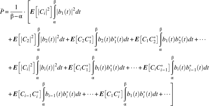
Consider a basis set {b1, b2, …} for the interval [α, β], where the basis signals do not necessarily form an orthogonal set. With such a basis set, each signal in the signal sample space of a random process ![]() has the decomposition
has the decomposition

and the kth coefficients define a random variable Ck with outcomes ![]() . Consistent with Equation 7.95, the average power, or average energy, in the random process is
. Consistent with Equation 7.95, the average power, or average energy, in the random process is
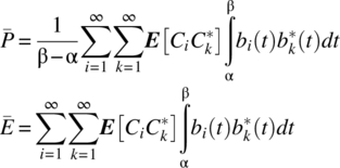
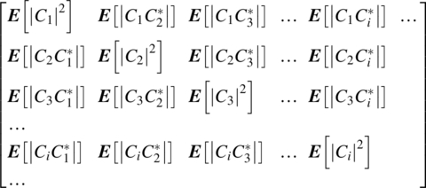
The average power, or average energy, depends on the nature of ![]() ,
, ![]() , and it is useful to define the following correlation matrix:
, and it is useful to define the following correlation matrix:
7.6.2.3 Orthonormal Basis Set and Uncorrelated Coefficients
It has been shown (Theorems 7.9 and 7.10) that orthogonality of the basis signals and uncorrelatedness of the basis signal coefficients are sufficient conditions for the average power of a random process to equal the summation of the average power of the individual signal components. It is of interest if orthogonality of the basis signals is linked to the uncorrelatedness of the basis signal coefficients.
Consider an arbitrary orthonormal basis set {b1, …} and the decomposition for the ith signal defined by the random process ![]() , on the interval [0, T], according to
, on the interval [0, T], according to

The following theorem states sufficient conditions on the basis functions for uncorrelated coefficients.
7.6.2.4 Karhunen–Loeve Decomposition
For a set random process, with RXX(t, λ) known, solving Equation 7.112 for the basis functions results is a Karhunen–Loeve basis set.
7.7 CLASSIFICATION: STATIONARITY VS NON-STATIONARITY
A widely used classification of random phenomena is based on the concept of stationarity, and two definitions are important: strict-sense stationarity and wide-sense stationarity. The latter is widely used.
7.7.1 Definitions
To define strict-sense stationarity, first, consider two random processes defined on a sample space S and on the infinite interval ![]() :
:
Each signal defined by V is a time-shifted version of the corresponding signal from X.
7.7.1.1 Finite Interval
Wide-sense stationarity for the interval [0, T] implies

7.7.1.2 Stationary and Nonstationary Random Processes
Most random phenomena commencing at a set time, which exhibit an initial transient response, are nonstationary. Many random phenomena, which exhibit steady-state behavior after the transient period, will exhibit characteristics consistent with stationarity. A random walk, for example, is clearly nonstationary.
7.7.2 Examples of Stationary Random Processes
The following subsections detail random processes that are wide-sense stationary:
7.7.2.1 Example 1
Consider an random process ![]() defined by a sinusoid with random phase:
defined by a sinusoid with random phase:

which has the following properties:

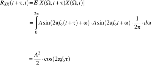
and is wide-sense stationary.
7.7.2.2 Example 2
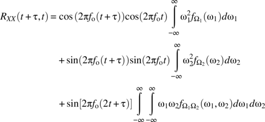
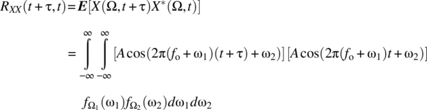
Consider the random process defined by the sum of two sinusoids of the same frequency but with random amplitudes:
where ![]() is a pair of random variables whose outcomes are governed by the joint probability density function
is a pair of random variables whose outcomes are governed by the joint probability density function ![]() .
.
The mean and autocorrelation functions are
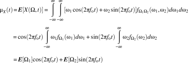

Multiplying terms yields
as
Thus,

and it then follows that the random process is wide-sense stationary if Ω1 and Ω2 have zero mean, have identical variances, and are uncorrelated, that is, ![]() ,
, ![]() , and
, and ![]() . Here, the result
. Here, the result
has been used. With the stated assumptions,
7.7.2.3 Example 3
Consider the random process defined by a sinusoid with random frequency variations around a set frequency and with random phase:
where ![]() is a pair of independent random variables with respective density functions
is a pair of independent random variables with respective density functions ![]() and
and ![]() .
.
The mean of this random process is

For the case where  , it follows that
 ![]() as required by stationarity.
as required by stationarity.
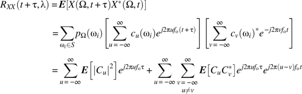
The autocorrelation function, by definition, is
As ![]() , it follows that
, it follows that

For the case where Ω2 has a uniform distribution on ![]() , it follows that
, it follows that
which is consistent with wide-sense stationarity.
7.7.3 Implications of Stationarity
Several important results can be stated for stationary random processes.
7.7.4 Wide-Sense Stationarity and Correlation of Coefficients
Consider a random process ![]() defined on the interval [α, β] and the Fourier series decomposition of each signal:
defined on the interval [α, β] and the Fourier series decomposition of each signal:
The coefficients define a set of random variables ![]() where the sample space of Ck is
where the sample space of Ck is ![]() . The following theorem states sufficient conditions for wide-sense stationarity (Koopmans, 1974/1995, p. 40):
. The following theorem states sufficient conditions for wide-sense stationarity (Koopmans, 1974/1995, p. 40):
7.7.4.1 Stationarity Implies Uncorrelated Fourier Coefficients
Theorem 7.15 states that if the coefficients defined by a Fourier series decomposition of the signals in a random process are uncorrelated and have zero mean apart from the zeroth-order coefficient, then the random process is wide-sense stationary. The converse is also true (Kawata, 1969; Papoulis, 1965, pp. 367, 461; Yaglom, 1962, p. 36).
7.8 CRAMER’S REPRESENTATION
Consider a random process ![]() defined on the interval [0, T] with
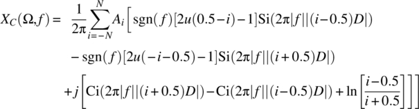
defined on the interval [0, T] with ![]() . Consistent with the discussion in Chapter 3, the Cramer representation of the signal X(ω, t), denoted XC(ω, f), by definition, is
. Consistent with the discussion in Chapter 3, the Cramer representation of the signal X(ω, t), denoted XC(ω, f), by definition, is

The set of signals ![]() defines the associated random process XC:
defines the associated random process XC:

The shorthand notation

is useful.
Using the signal definitions in Chapter 3, the following integrated spectrum, spectrum, and power spectrum definitions can be made.
7.8.1 Fundamental Results
The following theorems state fundamental results.
7.8.1.1 Notes
The first result of Theorem 7.18 implies that the integrated spectrum, XC(Ω, f), is an orthogonal increment random process on the infinite interval. This result does not hold for the interval [0, T] as ![]() .
.
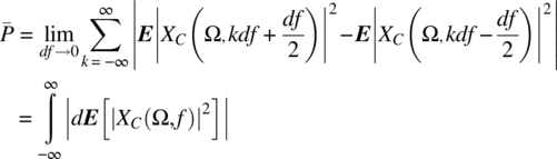
The second result of Theorem 7.18 states that the expected magnitude squared value of the difference in the integrated spectrum between f1 and f2 equals the power in the sinusoidal components with frequencies between the two values. This result justifies the definition of the power spectrum |dXC(f)|2, as given by Equation 7.152, as a valid power spectrum with a resolution of ![]() for the interval
for the interval ![]() . In summary:
. In summary:
7.8.1.2 Notes
Theorem 7.19 states that the expected mean squared change of XC(Ω, f), which is an orthogonal increment function, between f2 and f1 equals the change in the integrated power spectrum, that is, the power, between f2 and f1.
To determine the power spectrum, as given by |dXC(f)|2, it is sufficient to determine the integrated power spectrum as given by ![]() .
.
For the case where the integrated power spectrum is continuous, the power spectral density can be defined according to
7.8.1.3 Power
7.8.2 Continuous Spectrum
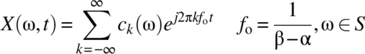
Consider any arbitrary interval of the form ![]() and a random process
and a random process ![]() ,which is such that all signals in SX can be decomposed, using a Fourier series, into the form
,which is such that all signals in SX can be decomposed, using a Fourier series, into the form

Such a decomposition leads to a discrete line power spectrum of the form shown in Figure 7.8. It is of interest if a random process exists, which has a spectrum with spectral components that are spaced arbitrarily closely, such that a continuous spectrum results.
Figure 7.8 Power spectrum as defined by a Fourier series.
7.8.2.1 Example of a Random Process with a Continuous Spectrum
Consider a sequence of random processes ![]() where the ith random process is defined according to
where the ith random process is defined according to

Here, B is a constant with the restriction ![]() , Θ is a continuous random variable with a uniform distribution on
, Θ is a continuous random variable with a uniform distribution on ![]() , and K is a discrete uniform random variable with a sample space
, and K is a discrete uniform random variable with a sample space ![]() and with
and with ![]() . The two random variables are assumed to be independent. For the ith random process, the waveforms are sinusoidal with frequencies randomly selected from the set
. The two random variables are assumed to be independent. For the ith random process, the waveforms are sinusoidal with frequencies randomly selected from the set ![]() , and associated with each waveform is random phase.
, and associated with each waveform is random phase.
For the ith random process, the expected power in the frequency range ![]() is determined by the power of a sinusoid with a frequency
is determined by the power of a sinusoid with a frequency ![]() , which occurs with a probability 1/2i. The expected power is
, which occurs with a probability 1/2i. The expected power is ![]() . The expected power in the interval
. The expected power in the interval ![]() equals the average power, which is A2/2.
equals the average power, which is A2/2.
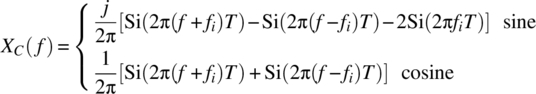
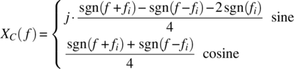
The Cramer transform of one outcome of the ith random process as specified by

is given, for the infinite interval ![]() , by (see Table 3.1)
, by (see Table 3.1)

Thus,

and

These functions are illustrated in Figure 7.9.

Figure 7.9 Graph of the magnitude of the Cramer transform and the power spectrum associated with Xi (k, θk, t).
The probability of each signal in the ith random process is 1/2i. It then follows that the power spectrum, ![]() , of the ith random process has the form illustrated in Figure 7.10.
, of the ith random process has the form illustrated in Figure 7.10.

Figure 7.10 Graph of the power spectrum for the ith random process.
7.8.2.2 Meaning of a Continuous Spectrum
For such a sequence of random processes, it is the case, for any fixed finite resolution in f of B/2i, that the random processes X1, …, Xi have a power spectrum with a discrete uniform distribution as illustrated in Figure 7.10. The power spectrum for the random processes ![]() will appear increasingly uniform and continuous when viewed with the same resolution.
will appear increasingly uniform and continuous when viewed with the same resolution.
7.8.3 Example: Binary Communication Random Process
Consider a random process that defines binary communication signals on the interval ![]() ,
, ![]() , according to
, according to

where ![]() ,
, ![]() , are identical and independent random variables with zero mean and variance
, are identical and independent random variables with zero mean and variance ![]() .
.
As detailed in Chapter 3 (Eq. 3.152), the Cramer transform of a unit step function ![]() on the interval
on the interval ![]() , assuming
, assuming ![]() and
and ![]() , is
, is

Hence,
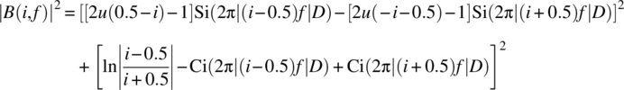
Define

and it follows that
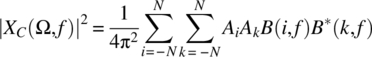
and the integrated power spectrum is

as ![]() when
when ![]() . Here,
. Here,
The power spectral density can then be evaluated according to
The integrated power spectrum is shown in Figure 7.11 for the case of ![]() ,
, ![]() , amplitudes from the set
, amplitudes from the set ![]() and
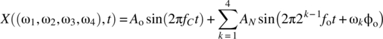
and ![]() . The corresponding power spectral density is shown in Figure 7.12.
. The corresponding power spectral density is shown in Figure 7.12.

Figure 7.11 Integrated power spectrum of a binary communication signal defined on the interval [−ND − D/2, ND + D/2] for the case of N = 16, D = 1, amplitudes from the set {−1,1}, and  .
.

Figure 7.12 Power spectral density of a binary communication signal defined on the interval [−ND − D/2, ND + D/2] for the case of N = 16, D = 1, amplitudes from the set {−1,1}, and  . G(f) is the power spectral density defined by the Cramer transform and evaluated with a frequency resolution of df = 1/2(ND + D/2). G∞(f) is the power spectral density assuming a sinusoidal basis set.
For reference, the power spectral density obtained according to
is as ![]() ,
,
where P(f) is the Fourier transform of the signalling pulse ![]() , that is,
, that is,
This power spectral density is shown in Figure 7.12.
7.8.3.1 Notes
The random process is not wide-sense stationary as is evident from the autocorrelation function

which is illustrated in Figure 7.13. This nonstationarity results in the power spectral density, as given by Equation 7.178, not being a valid power spectral density in terms of the usual requirement of the sum of the power in the individual components being equal to the total power. The next section details a stationary random process (white noise) whose power spectral density defined by the Cramer transform is a power spectral density that satisfies such a requirement.

Figure 7.13 Autocorrelation function of the defined binary communication random process.
7.8.4 White Noise: Approach II
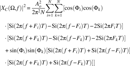
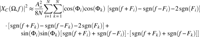
Consider a white noise random process ![]() defined according to
defined according to
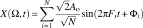
where ![]() , F1, …, FN are independent random variables with a uniform distribution on [0, fmax], Φ1, …, ΦN are independent random variables with a uniform distribution on the interval
, F1, …, FN are independent random variables with a uniform distribution on [0, fmax], Φ1, …, ΦN are independent random variables with a uniform distribution on the interval ![]() , and N is fixed according to
, and N is fixed according to ![]() where fo is the nominal frequency resolution.
where fo is the nominal frequency resolution.
7.8.4.1 Example
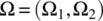
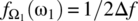
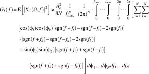
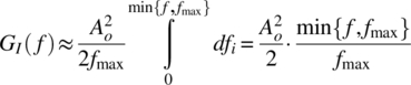
In Figures 7.15 and 7.16, the integrated power spectrum as given by Equation 7.184 and the associated power spectral density as given by
are shown for the finite interval case with ![]() ,
, ![]() , and
, and ![]() and an average signal power of
and an average signal power of ![]() .
.

Figure 7.15 Integrated power spectrum for a white noise random process defined on the interval [−T, T] for T = 10, Ao = 1, and fmax = 1.
Figure 7.16 Power spectral density for a white noise random process defined on the interval [−T, T] for T = 10, Ao = 1, and fmax = 1. A resolution of df = 1/2T has been used.
7.9 STATE SPACE CHARACTERIZATION of Random Processes
In some instances, the time nature of a random process is less important than the states that the random process takes on, and for this case, Markov theory is often appropriate (Allen, 1978, p. 129f; Grimmett and Stirzaker, 1992, p. 156f).
7.9.1 Markov Processes
Markov processes are characterized by a lack of memory: the future is dependent on the current state of the random process and not on its past. The theory of Markov processes can be applied to queueing systems, population dynamics, diffusion processes, probability of error calculations in communication systems, etc.
7.9.1.1 Classification of Markov Processes
As noted in Chapter 5, one-dimensional random processes define signals that are either discrete time–discrete state, discrete time–continuous state, continuous time–discrete state, or continuous time–continuous state. Consistent with this demarcation, Markov processes can be classified as detailed in Table 7.1.
Table 7.1 Demarcation of Markov random processes
| State space | ||
| Discrete time–continuous time | Countable # states: Markov chain | Uncountable # states: Markov process |
| Countable → discrete time Markov process | Discrete time Markov chain | Discrete time Markov process |
| Uncountable → continuous time Markov process | Continuous time Markov chain | Continuous time Markov process |
7.9.1.2 Definition of a Markov Random Process
7.9.2 Discrete Time–Discrete State Random Processes
7.9.2.1 State Diagrams for Discrete Time–Discrete State Random Processes
Consider a discrete time–discrete state random process X defined on a sample space S according to

where the set ![]() specifies the times at which signals from the random process are defined, and at these times the signals take on values from the state space
specifies the times at which signals from the random process are defined, and at these times the signals take on values from the state space ![]() . The possible states are illustrated in Figure 7.17.
. The possible states are illustrated in Figure 7.17.

Figure 7.17 Left: illustration of the possible states for a discrete time–discrete state random process. Right: illustration of the possible transitions at the time tk.
At each possible time, a discrete random variable is defined. For the kth time, the random variable ![]() is defined along with the associated probability mass function:
is defined along with the associated probability mass function:
At the time tk, the transitions, as illustrated in Figure 7.17, are possible. For the time t1, the probabilities associated with these transitions form a matrix according to
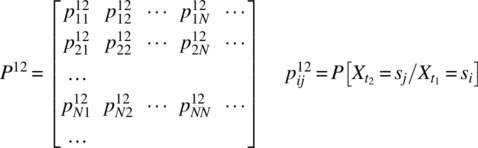
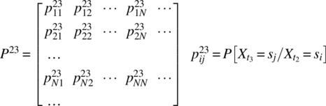
where the superscript of 12 indicates the transition as time changes from t1 to t2. At the time t2, the same transitions as at time t1 are possible but, in general, with different probabilities. For the special memoryless case—the Markov case—where the probabilities associated with these transitions are dependent only on the state level and not on the prior transition, the following transition probability matrix can be defined:
For the nonmemoryless case—the non-Markov case—the transition probabilities have the form
etc.
7.9.2.2 Characterizing a Trajectory of a Signal from a Random Process
The probability of a given trajectory for a random process over N possible transitions is

Expanding yields

For a Markov process, it then follows that

and a two-state transition matrix is sufficient.
7.9.3 Homogenous Markov Chain
7.9.3.1 Example: Random Walk
A random walk, X, with states ![]() and with transition probabilities
and with transition probabilities

is a homogenous Markov chain. The transition probability matrix is

7.9.3.2 Example: Ehrenfest Model
Consider m particles, as illustrated in Figure 7.18, that are distributed on either side of a membrane and that diffuse from one side to the other. When the probability of a particle diffusing from one side to the other side is proportional to the number of particles on the first side, the Ehrenfest model is defined. Consider a random process X defined as the number of particles on the right side of the membrane. An increase in X from a level i is consistent with one of the ![]() particles moving from the left side to the right side and a decrease in X from a level i is consistent with one of the i particles moving from the right side to the left side. With the Ehrenfest model, the transition probabilities, for
particles moving from the left side to the right side and a decrease in X from a level i is consistent with one of the i particles moving from the right side to the left side. With the Ehrenfest model, the transition probabilities, for ![]() are
are


Figure 7.18 Diffusion of particles from one side of a membrane to the other side.
The random process X is a homogenous Markov chain with a transition probability matrix:

7.9.4 N-Step Transition Probabilities for Homogenous Case
For a homogenous Markov chain, the following definitions can be made.
7.9.4.1 Chapman–Kolmogorov Equation
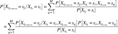
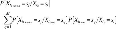
Consider the possible paths between the ith state at time tk and the jth state at time ![]() as illustrated in Figure 7.19.
as illustrated in Figure 7.19.

Figure 7.19 Possible paths for a discrete time–discrete state random process between the ith state at time tk time and the jth state at time tk + m + n.
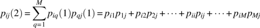
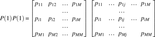
7.9.4.2 N-Step Transition Probability Matrix
7.9.4.3 Example
Consider an N-stage communication system, as illustrated in Figure 7.20, with identical stages and with binary data being transmitted. The probabilities characterizing each stage are
and define the transmission matrix illustrated in Figure 7.20. The input data is characterized according to
with ![]() .
.
Figure 7.20 Top: N-stage communication system. Bottom: transmission matrix for each stage.
An important measure of the communication system is the probability of error in transmission after N stages, which is defined as
A simple approach to finding the probability of error is to note that the communication link defines an N-stage homogenous Markov chain where each stage has two possible states with a transition probability matrix of

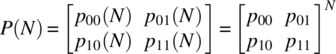
It then follows, from Theorem 7.24, that the transmission probability matrix for N stages is
and the probability of error is
For the case of ![]() ,
, ![]() , and
, and ![]() , the probability of error is shown in Figure 7.21.
, the probability of error is shown in Figure 7.21.

Figure 7.21 Probability of error in a binary communication system as the number of stages varies.
7.9.5 PMF Evolution for Homogenous Markov Chain
For a homogenous Markov chain, the n-step transition probability matrix ![]() facilitates establishing the evolution of the probability mass function once the initial state probabilities are known. The initial states, associated with the time t0, define a random variable
facilitates establishing the evolution of the probability mass function once the initial state probabilities are known. The initial states, associated with the time t0, define a random variable ![]() with outcomes s1, …, si, … and a probability mass function
with outcomes s1, …, si, … and a probability mass function
The nth transition time, tn, defines a random variable ![]() with outcomes s1, …, si, … and a probability mass function
with outcomes s1, …, si, … and a probability mass function
This probability mass function is specified in the following theorem.
7.9.5.1 Example
Consider a one-step processing system, as illustrated in Figure 7.22, with one level of redundancy such that the state diagram, as detailed in Figure 7.23, is appropriate. The state diagram arises from the state assignment detailed in Table 7.2. It is assumed that there is a time between when a unit fails and when it is taken for repair, and this time varies depending on the nature of the fault. It is also assumed that the repair time varies with the nature of the fault.

Figure 7.22 A one-step processing system with one level of redundancy. The router directs the input to unit one when it is operational and to unit 2 when unit 1 has failed.
Figure 7.23 State diagram for system. O, F, and R stand, respectively, for operational, fail, and repair.
Table 7.2 State assignment for the system of Figure 7.22
| State | Unit 1 | Unit 2 | System status |
| s1 | Operational, in use | Operational, standby | Operational |
| s2 | Failed | Operational | |
| s3 | Being repaired | Operational | |
| s4 | Failed | Operational, in use | Operational |
| s5 | Failed | Nonoperational | |
| s6 | Being repaired | Nonoperational | |
| s7 | Being repaired | Operational, in use | Operational |
| s8 | Failed | Nonoperational | |
| s9 | Being repaired | Nonoperational |
For the case where the system state is updated at set rate of 1/Δt, the transition probability matrix is

The following definitions, associated with a time interval of duration Δt seconds, apply: pF is the fault probability given initial operation status, pFR is the probability of moving to a repair state given an initial failed status state, and pRO is the probability of moving to an operational state given an initial repair state. With these definitions, it then follows that
The evolution of the state probabilities with time, as given by P0Pn(1), is shown in Figure 7.24 for the case of ![]() (an unrealistically high value but a value that demonstrates the nature of the state probability evolution),
(an unrealistically high value but a value that demonstrates the nature of the state probability evolution), ![]() ,
, ![]() , and
, and ![]() .
.

Figure 7.24 Probability mass function evolution with the number of time intervals of duration Δt. Here, tn = nΔt.
Of interest is the probability that the system is operational. At the time ![]() , this is given by (see Table 7.2)
, this is given by (see Table 7.2)
The evolution with time of the probability of the system being nonoperational is shown in Figure 7.25 for the case of ![]() ,
, ![]() ,
, ![]() , and
, and ![]() .
.

Figure 7.25 Probability of system being nonoperational for the case of pF = 0.0001, pFR = 0.4, pRO = 0.33, and tn = nΔt.
7.9.6 First Passage Time for Homogenous Markov Chain
The follow definitions underpin the determination of characteristics related to a state being reached for the first time.
7.10 TIME SERIES CHARACTERIZATION
Time series characterization is an important area, and AR, MA, and ARIMA models find widespread application. Brillinger (2001), for example, provides a good introduction.
7.11 PROBLEMS
- 7.1 Consider an experiment with a sample space
 and where the probability of an outcome is specified by the probability mass function
  . A random process is defined on the experiment according to
(7.232)
. A random process is defined on the experiment according to
(7.232)
- Explicitly define SX.
- Define the following associated random processes:
- The random process defined by the autocorrelation function
- The random process defined by the time-averaged autocorrelation function
- The random process defined by the Fourier transform
- The random process defined by the power spectral density function
- Determine the time-averaged autocorrelation function and the power spectral density function for the random process.
- Show that the Fourier transform of the time-averaged autocorrelation function equals the power spectral density.
- Determine the average power of the random process. Show that the average power equals the value of the time-averaged autocorrelation function with an argument of zero and is also equal to the integral of the power spectral density function.
Note that
 (Gradsteyn and Ryzhik, 1980, eq. 0.241.)
 - 7.2 Consider a system, where on power down, a transient signal component is evident. This is modelled by the random process
 according to
(7.233)
according to
(7.233)
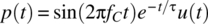
for a causal pulse function p.
- Determine the mean and variance of the random process.
- Determine an expression for the probability density function evolution with time of the random process.
- For the case of
 ,
,  ,
,  , and
, and  , graph the mean, variance, and probability density function evolution with time.
- 7.3 Consider a sinusoidal signal with a phase component that is randomly varying and that can be approximated by a random walk. The set of possible sinusoids defines a random process according to
(7.234)
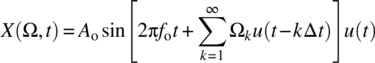
where
 and Ω1, Ω2, … are independent and identical random variables with a sample space
  and with
  . The following result is useful: for a random walk with a step size of Δx, after N steps, the possible levels are
  and the probability of the level kΔx is
- Determine analytical expressions for the mean, mean squared value, and variance of the random process.
- Determine an analytical expression for the autocorrelation function of the random process. To determine the joint probability mass function of the random walk at the times t and
 , it is useful to use the result(7.235)
- Note that the expressions for the mean, variance, and autocorrelation function allow the correlation coefficient of the random process at the times t and
 to be determined.
 -
For the case of
 ,
,  ,
,  , and
, and  , graph examples of the phase variation with time, and graph the variation with time of the mean and variance. Graph the autocorrelation and correlation coefficient with respect to time and the delay τ. By varying Δt and φo, the duration of the transient period, before the random process becomes approximately stationary, can be ascertained.
- 7.4 Consider the case of a sinusoidal signal that is corrupted by additive noise such that a random process
 results:
(7.236)
results:
(7.236)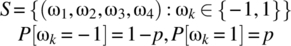
- For the case of
 ,
,  ,
,  ,
,  , and
, and  , graph some of the possible signals, and the noise components, from the random process.
 - Determine the average power of the signals in the random process and the average power of the random process. Assume an interval T that is an integer multiple of 1/fo.
- Establish expressions for the coefficients in the decomposition(7.237)

on the interval [0, 1/fo] for the case of
 . Hence, determine the average power of the random process as a summation over the expected value of the magnitude squared of the coefficients.
- For the case of
- 7.5 Consider a random process
 defined according to
(7.238)
defined according to
(7.238)
where C1 and C2 are random variables defined on S.
- Determine general expressions for the mean and autocorrelation function of the random process.
- If C1 and C2 are uncorrelated, then specify the autocorrelation function.
-
Consider the case of
 ,
,  , and
, and  and where the sample spaces of the random variables C1 and C2, respectively, are
  and
and  . Show that C1 and C2 are uncorrelated. Determine expressions for the mean and autocorrelation functions for this case. Is the random process stationary? What nonzero functions b1 and b2 would ensure stationarity?
 - Using the above specified parameters and assuming (7.239)

graph the autocorrelation function for the case of
 .
.
- 7.6 Consider an experiment with a sample space
(7.240)

and with outcomes governed by a joint probability density function
(7.241)
A random process
 is defined on this sample space according to(7.242)
for defined functions g1 and g2.
- Determine general expressions for the mean, variance, and autocorrelation function of the random process.
For the following parts, consider the specific definitions:
(7.243) (7.244)
- Determine expressions for the mean, variance, and autocorrelation function.
- For the case of
 ,
,  , and
, and  , graph signals from the random process.
 - For the above defined parameters, graph the mean, variance, autocorrelation function, and correlation coefficient.
- For the above defined parameters, graph the effective correlation time for
 .
. - For the above defined parameters, graph the expected mean squared change.
- Determine general expressions for the mean, variance, and autocorrelation function of the random process.
- 7.7 A random process X is based on an experiment with outcomes
(7.245)

and where the outcomes are governed by the probability density function
 ,
,  ,
,  , and
, and  . The random process is defined according to(7.246)
- Determine the mean and autocorrelation function of this random process, and confirm that it is a wide-sense stationary random process.
- Using the Cramer transform, determine the integrated spectrum and integrated power spectrum for the random process. For the latter, leave your result in an integral form.
- For the case of
 ,
,  ,
,  , and
, and  , use numerical integration to graph the integrated power spectrum and the associated power spectral density.
- 7.8 Consider the case of a progressive disease in a specific species with no known cure but with several effective treatments. The initial treatment is available when the disease is diagnosed and classed as being in stage 1. When the disease is classed as being in stage 2, a second treatment is available. When the disease is classed as being in stage 3, only new experimental treatments are available. The disease is such that the initial treatment is not effective a second time. The state diagram, as detailed in Figure 7.26, is appropriate. The state diagram arises from the state assignment detailed in Table 7.3. The transition probabilities listed in Figure 7.26 are for a specified time interval.
- Specify the transition probability matrix.
- Graph the time evolution of the state probabilities assuming state 1 at
 .
. - Determine the probability that an entity from the species, chosen at random, has not been diagnosed with the disease, is in stage three of the disease, or has died after 10, 20, and 100 time intervals.
Figure 7.26 State diagram for disease progression and state transition probabilities.
Table 7.3 State assignment for states defined in Figure 7.26
State Definition s1 Prior to initial disease diagnosis s2 Stage 1 of disease s3 First treatment s4 Remission phase s5 First treatment unsuccessful s6 Stage 2 of disease s7 Second treatment s8 Stage 3 of disease s9 Experimental treatment s10 Death
APPENDIX 7.A PROOF OF THEOREM 7.2
The proof is given for the countable case; the proof for the uncountable case follows in an analogous manner. First, ![]() guarantees the existence of
guarantees the existence of ![]() . As
. As ![]() implies
implies ![]() (Theorem 2.13), it follows that the Fourier transform of X(ωi, t), denoted X(ωi, T, f), exists, and thus, G(ωi, T, f) is well defined.
(Theorem 2.13), it follows that the Fourier transform of X(ωi, t), denoted X(ωi, T, f), exists, and thus, G(ωi, T, f) is well defined.
For the time-averaged autocorrelation function, consider the case of ![]() :
:
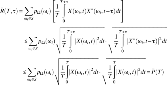
where Schwarz’s inequality (Theorem 2.15) has been used. Thus, the assumption of finite average power implies that ![]() is finite for
is finite for ![]() , which implies
, which implies ![]() .
.
For the power spectral density, the assumption of finite average power implies:

Here, Parseval’s relationship (Theorem 3.9) has been used. The interchange of the summation and integral is valid, from the Fubini–Tonelli theorem (Theorem 2.16), as all terms are positive and the summation of the integral exists by the assumption of finite average power. Thus,  , which implies
 ![]() and, hence, the existence of G(T, f) for all f except, potentially, at a countable number of points.
and, hence, the existence of G(T, f) for all f except, potentially, at a countable number of points.
APPENDIX 7.B PROOF OF THEOREMS 7.3 AND 7.4
7.B.1 Autocorrelation Function: Theorem 7.3
Consider the countable case: by definition
Convergence is guaranteed as
has assumed to be finite. This assumption also ensures that the interchange of the limit and summation, consistent with the dominated convergence theorem (Theorem 2.19), is valid, that is,
As shown in Appendix 7.A, ![]() is finite if
is finite if ![]() , and the average power in the random process
, and the average power in the random process ![]() is finite. These results extend to the infinite interval when
is finite. These results extend to the infinite interval when ![]() for all
for all ![]() ,
, ![]() , and when there is an upper bound on the signal powers over the interval
, and when there is an upper bound on the signal powers over the interval ![]() as specified by Equation 7.71.
as specified by Equation 7.71.
7.B.2 Power Spectral Density: Theorem 7.4
Consider the countable case:
Finiteness of ![]() is guaranteed as
is guaranteed as
has been assumed. This assumption also ensures the validity of the interchange of the limit and summation, according to the dominated convergence theorem (Theorem 2.19), i.e.,
A sufficient condition for G(ωi, T, f) to be bounded as ![]() is for
is for ![]() . A stronger condition can be found by considering
. A stronger condition can be found by considering
Hence, if ![]() , then G(ωi, T, f) is bounded.
, then G(ωi, T, f) is bounded.
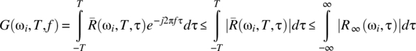
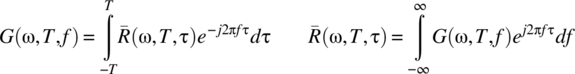
APPENDIX 7.C PROOF OF THEOREM 7.5
First, consistent with Theorem 3.14, the assumption of finite energy, and piecewise differentiability, on [0, T] for each signal, ensures that
for all ![]() . Consider the countable case: to prove that the power spectral density is the Fourier transform of the time-averaged autocorrelation function, consider the integral
. Consider the countable case: to prove that the power spectral density is the Fourier transform of the time-averaged autocorrelation function, consider the integral

Consistent with Theorem 7.2, the assumption of finite average signal power on [0, T] implies that the summation is bounded above, that is, ![]() is finite. It then follows from the Fubini–Tonelli theorem that the order of the summation and the integral operation can be interchanged to yield
is finite. It then follows from the Fubini–Tonelli theorem that the order of the summation and the integral operation can be interchanged to yield
To prove that the inverse Fourier transform of the power spectral density function equals the time-averaged autocorrelation function, consider

Consistent with Theorem 7.2, the assumption of finite average signal power on [0, T] implies that the summation is bounded above, that is, G(T, f) is finite and, further, ![]() . It then follows from the Fubini–Tonelli theorem that the order of the summation and the integral operation can be interchanged to yield
. It then follows from the Fubini–Tonelli theorem that the order of the summation and the integral operation can be interchanged to yield
As ![]() is finite for all values of τ, it follows that
is finite for all values of τ, it follows that
APPENDIX 7.D PROOF OF THEOREM 7.6
First, the assumed conditions, consistent with Theorem 7.5, ensure that the ![]() and G(T, f) exist for all
and G(T, f) exist for all ![]() and that they are related via the Fourier and inverse Fourier transforms.
and that they are related via the Fourier and inverse Fourier transforms.
To relate ![]() to
to ![]() , consider
, consider

It is necessary to interchange the limit and integration operations in this equation. To achieve this, first, note, consistent with Theorem 7.2, that ![]() . Second, assume there exists a function
. Second, assume there exists a function ![]() such that
such that ![]() for all T. Then, from the dominated convergence theorem (Theorem 2.19), it follows that the order of limit and integral can be interchanged to yield
for all T. Then, from the dominated convergence theorem (Theorem 2.19), it follows that the order of limit and integral can be interchanged to yield
To relate ![]() to
to ![]() , consider
, consider

Again, it is necessary to interchange the limit and integration operations. However, and in general, the power spectral density function G(T, f) will have impulsive components, and it is not possible to justify the interchange of the limit and integral operations. With the assumption of the existence of a function ![]() such that
such that ![]() for all T, it follows, from the dominated convergence theorem (Theorem 2.19), that the order of limit and integral can be interchanged to yield
for all T, it follows, from the dominated convergence theorem (Theorem 2.19), that the order of limit and integral can be interchanged to yield
APPENDIX 7.E PROOF OF THEOREM 7.11
Assume the countable case and consider ![]() :
:

A change of variable ![]() for λ results in the area for integration as illustrated in Figure 7.6. The expectation can then be written as
for λ results in the area for integration as illustrated in Figure 7.6. The expectation can then be written as

Define IR as

It then follows that

which clearly converges to zero as ![]() .
.
APPENDIX 7.F PROOF OF THEOREM 7.12
Consider the double summation consistent with the average power:

Expanding the summation out yields
and the following requirement then follows for the off-diagonal terms to be negligible:

APPENDIX 7.G PROOF OF THEOREM 7.16
Consider the countable case:
The assumption of wide-sense stationarity implies that the second summation is independent of t. Due to the harmonic nature of the terms in this summation, this is only possible if
Expanding the exponential terms out gives the condition
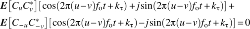
where ![]() . Due to the orthogonality of the sine and cosine functions, the requirement is for
. Due to the orthogonality of the sine and cosine functions, the requirement is for
and, hence, the condition that ![]() for
for ![]() .
.
APPENDIX 7.H PROOF OF THEOREM 7.17
Consider the countable case:
For the interval ![]() , the Cramer transform of
, the Cramer transform of  (see Theorem 3.29) is

and the approximation to this equation is

Thus,

For the stationary case ![]() when
when ![]() (see Theorem 7.16) and, thus
(see Theorem 7.16) and, thus

The exact expression follows in an analogous manner and is
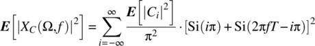
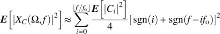
In Figure 7.27, the graph of ![]() is shown. It then follows that
is shown. It then follows that

Figure 7.27 Graph of [sgn (i) + sgn (f − ifo)]2. Left: i < 0. Right: i > 0.
APPENDIX 7.I PROOF OF THEOREM 7.18
Denote ![]() and consider the countable case:
and consider the countable case:
For an interval ![]() ,
, ![]() , it follows, from Theorem 3.32 for the case of
, it follows, from Theorem 3.32 for the case of ![]() , that
, that

It then follows, for the case of ![]() , that
, that
Interchanging the order of summations yields
Wide-sense stationarity implies, consistent with Theorem 7.16, that ![]() for
for ![]() , and it then follows that
, and it then follows that ![]() as
as ![]() ,
, ![]() , as required.
, as required.
It also follows from the result ![]() for
for ![]() , and for the case of
, and for the case of ![]() , that
, that

assuming f1 and f2 are integer multiples of fo. Consider the result from Theorem 7.17 for ![]() :
:
which, for ![]() , implies
, implies
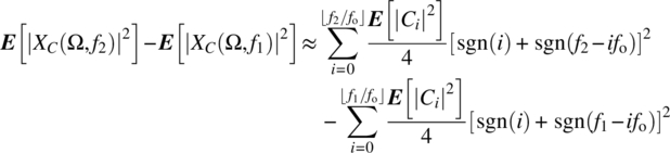
Thus,

assuming f1 and f2 are integer multiples of fo. As ![]() ,
, ![]() , and the significance of an individual term in the summation becomes increasingly small, it then follows from Equations 7.288 and 7.291 that
, and the significance of an individual term in the summation becomes increasingly small, it then follows from Equations 7.288 and 7.291 that

as required.
APPENDIX 7.J PROOF OF THEOREM 7.20
Consider the countable case and the definition of power:

Interchanging the order of summations, it follows that
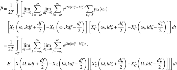
For ![]() and the same step size for df and dζ, it is the case, consistent with Theorem 7.18, that
and the same step size for df and dζ, it is the case, consistent with Theorem 7.18, that

Hence,
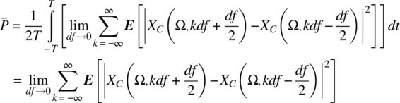
From Theorem 7.18, it then follows that
which is the required result.
APPENDIX 7.K PROOF OF THEOREM 7.21
Consider the alternative trigonometric form for X(Ω, t):

The Cramer transforms, respectively, of sin(2πfit) and cos(2πfit) for the interval ![]() are specified in Theorem 3.28:
are specified in Theorem 3.28:
and for the infinite interval (Theorem 3.27):
For the case of ![]() , the infinite interval result is a good approximation.
, the infinite interval result is a good approximation.
The associated random process defined by the Cramer transform of each signal of X(Ω, t) is
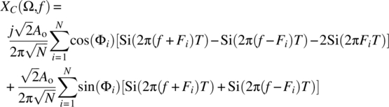
and this random process can be approximated according to

The associated random process defined by the magnitude squared of the Cramer transform of each signal of X(Ω, t) is
and this random process can be approximated according to
The joint density function of F1, …, FN, Φ1, …, ΦN is

and it then follows that
Interchanging the order of integrations and summations, and splitting the summations into the diagonal and nondiagonal components, yields
where


As the integral of a sinusoid over its period is zero, it is the case that ![]() . Further, as the integral of cos(φi)2 or sin(φi)2 over [0, 2π] equals π, it follows that
. Further, as the integral of cos(φi)2 or sin(φi)2 over [0, 2π] equals π, it follows that

The same procedure leads to the true form

The functions ![]() and
and ![]() have the graphs shown in Figure 7.28, and it then follows, for
have the graphs shown in Figure 7.28, and it then follows, for ![]() , that
, that
and ![]() . The power spectral density then is
. The power spectral density then is


Figure 7.28 Left: graph of sgn (f + fi) − sgn (f − fi) −2 sgn (fi). Right: graph of sgn (f + fi) + sgn (f − fi). The case of f > 0 is assumed.
APPENDIX 7.L PROOF OF THEOREM 7.23
Consider the following two results: first, from conditional probability theory,

Second, from the Theorem of Total Probability,

The substitution of Equations 7.313 into 7.312 yields
The Markov property of transition probabilities depending on the present, and not past, values results in
The substitution of this result, and the use of conditional probability theory, yields
as required.
APPENDIX 7.M PROOF OF THEOREM 7.24
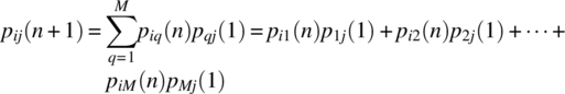
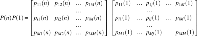
The proof is by induction. First, the theorem is true for the case of ![]() . Second, consider
. Second, consider ![]() . From the Chapman–Kolmogorov equation, it is the case for an M-state random process that
. From the Chapman–Kolmogorov equation, it is the case for an M-state random process that
Now,
and it is clear that the ijth element of this matrix is consistent with Equation 7.317, and the theorem holds for the case of ![]() . Third, consider the case of
. Third, consider the case of ![]() ,
, ![]() . From the Chapman–Kolmogorov equation, it follows that
. From the Chapman–Kolmogorov equation, it follows that
It is the case that
and it is clear that the ijth element of this matrix is consistent with Equation 7.319, and the result ![]() holds. Finally,
holds. Finally,
concludes the proof.