
Alan Turing first proposed the state machine in 1936. He envisaged a box with a paper tape input (input alphabet), a set of states (and start states), and a mechanism for mapping the input to the next state.
Definition—. A state machine is a conceptual machine with a given number of states; it will only be in one of the states at any given time. State transitions are changes in state caused by input events. In response to an input event the system may transition to the same or a different state, while an output event may be optionally generated.
For our purposes Enumerated Types and other assorted inputs replace the paper tape input. The mechanism for setting the start states is an initialization function, and the mechanism for mapping an input to the next state is the case structure. If the state machine needs to manage its own data you will need to include a While Loop structure and a shift register.
If you are beginning to think this is a little archaic, you could always call your state machine an object, package, module, component, or whatever.
So let's try out a simple and reasonably useless example before diving into the good stuff.
The standard example given to describe a state machine is the washing machine, so who are we to buck a trend. Figure 6.1 shows the states available to a washing machine.
Select your start state and run. It's best to view the diagram with Highlight Execution selected. If the subVIs are set up to run properly, you will find that the display light emitting diodes (LEDs) will run in order, displaying the current state of the washing machine.
Figure 6.2 is the hierarchy of subVIs, each one can be selected and its output condition chosen.
So looking at the block diagram in Figure 6.3 the start condition “Door Closed” is input into the shift register and then is passed to the case statement. The door state is returned (this could be from a switch reading) and then if the door is closed, the next state “Fill with Water” is called and so on.
The other states are modeled in Figure 6.4.
If you want to experiment with the actual state responses, pop up on the relevant subVI and change the enumerated settings control.
The corresponding state transition diagram is shown in Figure 6.5. The states are the boxes and the transitions are the arrows.
So why are state machines better than flowing it in the normal LabVIEW way?
The strictly sequential way in Figure 6.6 looks okay from a diagrammatic point of view, nice and simple, but what if we want to add a new state? Or change the order of states? Both of these would involve deleting the source code and moving VIs around. You don't have the options and control of flow that you get with the state machine structure.
The error handling is also more vague. If you model the error conditions as valid states of the system you will know what error was called, and you would also know that only the actions you control would be called on an error.
State machines are an excellent method of reducing complexity in your software. They allow your code to be flexible, readable, and maintainable.
Most of us initially have problems with UI implementation and controls in LabVIEW. They can end up having large, flat block diagrams or the use of globals (elegant, but a coupling and information hiding no-no). Some LabVIEW gurus suggest using globals as the only way to program complex LabVIEW UIs. They are WRONG! This section will demonstrate how you can view your Front Panel as a container of Controls that have Attributes and Actions associated with them. It would be nice if these Attributes and Actions could be triggered from anywhere in your applications hierarchy. Well, why not pass them as messages in a queue. Then, on your Front Panel you could read these items off the queue and respond to them. This is classic message sending. In effect, you are changing your UI into a state machine and queuing its new states. Figure 6.7 demonstrates this queuing mechanism.
Let's run through an example.
The Front Panel in Figure 6.8 is a simple demonstration of the principles discussed above. We will populate it with a few Indicators and Controls and then control them by queuing messages.

Either the graph or the table will be visible depending on the graph/table button condition as shown in Figure 6.8. Pressing the LED buttons will toggle the corresponding LED. In the background, the status string updates. This User Interface has minimal complexity, but you could add 10 times the complexity without changing the program structure markedly.
A list of what you want to do to it is shown in Figure 6.9.
As you can see, the UI states have already been typed into an enumerated type, allowing us to edit and remove items at will. Just pop up on the enumerated type and add the new function, its attributes, and update the UI control VI.
This is something you could sit down with your customer and define.
This enumerated type becomes the command for the wrapper VI that passes all the messages into the queue (UI Control.vi).
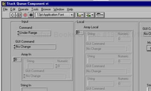
This little component, shown in Figure 6.10, is useful for many purposes. We tend to adapt it the most for Front Panel control, background filing, and database work. Figures 6.11, 6.12, 6.13 and 6.14 demonstrate how it functions.
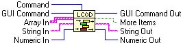
There are also several useful utilities for reading the top and bottom and checking if the component is empty. Here is the implementation in LabVIEW 6.
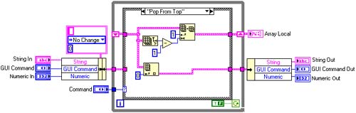
Selecting “Add to Top” or “Add to Bottom” on the enumerated type “GUI Command” shown in Figure 6.15, will pass the data into Array Local, either at the beginning or end of the array. You then have the option of taking this data from the beginning or end of the array with the commands “Pop from Top” or “Pop from Bottom”. Figures 6.16 and 6.17 show its implementation.
It's relatively easy to modify the component to your own data requirements by changing the inputs, clusters, and array contents to suit. Make sure that the source code is left the same though.
We'll use this component to store and transmit the states of the User Interface.
The stack queue component works fine for small queues, but if you want to beef up the performance you could try using the queue VIs that come with LabVIEW. In LabVIEW 6.1, NI very kindly made them polymorphic and they work nicely, giving a significant performance improvement. We rewrote the component to include these VIs and they were about eight times as fast for large queues (2,000+ elements).
How to get to the queue functions can be found in Figure 6.18.
We've kept the functionality and the interface similar, although there are now error clusters in and out. You can only take items from the end of the queue—a small sacrifice for the speed advantage. The element cluster is a strict type def, therefore, to reuse the queue all you have to do is customize the element cluster. This can be done using the queue VIs in earlier versions of LabVIEW, but you have to squish the data to a string and unsquish it afterwards. Also you lose the ability to use the component like a stack, the queue functions constrain you to queuing in one end and out the other.
The source code for this implementation is in Figure 6.19.
Next you have to create the wrapper component that conducts all the actions on the stack. For improved maintenance you could map the input command directly to the “GUI Command Out”, but this has a negative effect on the flexibility of the design. Figures 6.20, 6.21, and 6.22 describe the implementation for this VI.
Looking at Figure 6.21 you can see the case for the display state, “Set Table Graph Button Name”. When this command is selected and the VI executed the corresponding command and string are placed in the queue. A loop in the UI block diagram is then responsible for pulling the commands and settings off the queue and executing them. The case, “Get UI Setting” in Figure 6.22 is responsible for this.
Adding a new User Interface attribute or action is merely a matter of updating the enumerated type, duplicating the case, and changing the enumerated type in the case to suit.
Now put in the state machines for monitoring User Interface updates and checking for button presses. You will also notice in Figure 6.23 that everything is enclosed in another state machine that describes the states for the User Interface (initialize, run, finish).
You then fill out the “Monitor for UI Changes” state machine for all of the attribute settings and actions as shown in Figure 6.24.
As you can see, all the attributes and actions for the User Interface are held in a nicely documented case structure. Adding more functionality is just a matter of creating another pigeonhole and placing the control or property node into it.
You can also make a small test stub VI that pushes actions onto the queue, allowing you to test each individual display setting. Just drop the UI Control into a new VI and set each input as a control. Run your User Interface and on the test stub select the action you require and run the test stub. As if by magic, the UI will do your bidding.
What does “Abstraction in the code, detail outside the code” mean? Well, essentially the software should encapsulate the services that are to be provided, but there should not be any detail in the code. What?
To make this clearer we'll define what we mean by detail. Detail would be a GPIB address, measurement parameters, switching connections, and so on. The abstraction would be the component that provides the interface to the instrument at that address, the component that commands the instrument that makes the measurement, and the component that commands the switching.
Here is an interesting fact that we have noticed (that it is something we have noticed probably means it is not a fact, but go with it). When software is beyond the initial construction stages, it's the strings and integers that are changed more than the actual code. This is a double-edged sword because if you design the software with this rule in mind, you also produce code that is better designed, more flexible, more reusable, loosely coupled, and hence, easier to maintain.
Okay, this sounds a bit soapbox, so here is the golden rule:
When you look at your VIs, every time you see a number or string it should be taken out and placed in a file or database, yes, every single one of them!
We're serious. Think about it, every string and number in your code is detail, and detail changes. The GPIB address changes, the frequency span of your measurement changes, and the switching changes with a design change or addition of new hardware—these are all detail. But, the abstraction doesn't change. The instrument can be at any address, the address does not change how the component operates, a frequency measurement is the same regardless of the span, and switching is the same operation regardless of the location. As a simple illustration, your program is compiled to an exe and the hardware GPIB address has to change because of a clash somewhere, all you have to do is change the detail in a file (maybe a configuration file), no code changes, no recompiling. At the other extreme, the GPIB addresses are spread through the four corners of your code. If you change the address, then you have to hunt down all the occurrences—miss one and your application will fall over!
So, here's an example. Your application uses an analogue I/O board, and you want to measure data coming in on the analogue input (AI) channel. Now we have a nicely designed component that measures what we want, as shown in Figure 6.25.
But, we can see that the VI has DETAIL in it! The detail is the channel limits (array of clusters 5/–5), device (1), and channels. If for any reason this changes we have to change the code, which is exactly what we want to avoid.
So, an updated version is shown in Figure 6.26.
We can see that there are no longer any constants in our code, they have been replaced by three instances of the VI called Config. Simply put, the Config VI has the detail stored in a file outside the code.
As with most things in this book this seems simple. So, all detail in files or databases, okay that's easy. But bear in mind there will be huge dividends gained by adhering to this general rule. However, the simple thing to do is put the detail in the code with the mental note that you will take it out later (we know this because we're tempted every time). Multiply this by 500 VIs and you've missed the boat. Therefore, when you recognize detail, stop and put it outside the code. In the short term this becomes a little monotonous, but soon most of the data will be extracted and you will just reference it in later VIs.
You will need a place to store all of the detail data previously discussed, and we've found an ideal solution in section keyed files. There is a set of useful functions available on the function palette for implementing these files, as shown in Figure 6.27.
What is a section key file? It's the old .ini file as used by Windows 3.1, and it is a Text file with the following format:
[section name]
key1=Data1_1|Data1_2|Data1_3
key2=Data2_1
key3=Data3_1
The data held in these files is essential to the running of your application, therefore, there is an issue of security to consider, we don't want anyone coming and idly fiddling with the data held in these files. The configuration file functions as they stand do not give any encryption facilities, so as a first step let's add some.
All we need to do is replace “Config Data Read From File.vi” and “Config Data Write To File.vi” in “Close Config Data.vi” and “Open Config Data.vi” with encrypted versions and save them under a different name.
Let's do it step by step.
First open “Open Config Data.vi” from the functions palette and save it as “Encrypted Open Config Data.vi” as in Figure 6.28.
Open up the block diagram and double-click on “Config Data Read From File.vi”, as shown in Figure 6.29 and Figure 6.30.
Rip out all of the file opening and reading stuff and replace it in Figure 6.31.
So, we read the file as a bunch of integers and push them through an encryption component that decodes them. The encryption VI does some rotating and math on the incoming integers.
That's the data decoded when we read it. Now, let's finish it off by encrypting the file. If all the data is read when the config file is opened it stands to reason that it is saved when the file is closed. In a similar fashion to what we have just done, open “Close Config Data.vi”, as shown in Figure 6.32. Then, double-click on “Config Data Write To File.vi”, as shown in Figure 6.33.
Once again replace all the writing to file stuff with the encryption component as in Figure 6.34.
If you don't want to go through all of this you could always swipe the code off the Web site.
It would be ideal if we could add items to these files as we go along, developing our application without incurring a large programming overhead. What we need is a component that handles all of this for us.
By using Strict Type Def enumerations as keys and another Strict Type Def enumeration as the section, the following component allows items to be added simply by updating the relevant enumerated type. It encapsulates all of the functionality required for loading, saving, and editing data in section key files.
So, here's a list of the functionality.
Action | Description |
|---|---|
Invalid: | This is the default condition and should throw an error |
Get: | Returns the selected data item |
Set: | Sets the selected data item |
Save: | Saves the selected data item to file |
Load: | Loads the selected data item from file |
Save All: | Saves everything to file |
Load All: | Loads everything from file |
Reset: | Clears out local memory manually |
Storing the data in a shift register that is an array of clusters of arrays (?!?) works okay for reasonable amounts of data, and is simple to implement. For extravagant amounts of data you could store the data in a hashed array structure, or something similar. The interface stays the same no matter what method of organizing the data is employed (demonstrating the power of information hiding).
Let's briefly discuss each of the component actions and look at the implementation.
The Front Panel is shown in Figure 6.35.
To run the component, select the action [Command] and the attribute [Parameter], fill out the data in [String Array In] if required, and run it. There is a File Handler Component that will need setting up prior to filing operations, but this will need to be done only once. It holds the references to the systems files. We'll now describe the source code in detail.
The Invalid state, in Figure 6.36, should never be called and is only there to pick up development errors and mis-wires. If it does occur the software should throw a tantrum about it.
The code in the top left-hand part of the While Loop checks if the local array has been initialized, and if not, sets it to the number of parameters in the “Parameter” Enumeration. The two small cases open and close the files if the Command is file related. The middle case is where all the action is, and for the Invalid state it fires the Error Control into action, throwing up a dialog box moaning about being called and listing who called it.
Figure 6.37 shows the “Get” action. The relevant array is selected by using the index of the enumerated type, and output as a string and an array.
Figure 6.38 shows the “Set” action. Once again the new array is input at the index desired by the enumerated type “Parameter”. This new data is persistently stored in the shift register.
Figure 6.39 is the “Save” action. The array selected by the index of the “Parameter” enumerated type is stored in the section-keyed file at the key defined by the text of the “Parameter” enumerated type.
In addition to saving the data you will want to load it from the file as well. Figure 6.40 shows the “Load” action. The text of the “Parameter” enumerated type is again used as the key for selecting the data to pull from the file. The returned string is then converted to an array and inserted into the shift register at a location defined by the index of “Parameter” enumerated type.
Figure 6.41 demonstrates the “Save All” action. The “For Loop” will auto-index for every element in the shift register array, saving to the key produced from the “Strings[]” property of the “Parameter” enumerated type.
The “Load All” action shown in Figure 6.42 iterates through all the parameters, filling up the shift register array. The “File Handler” component holds all the file references and is also responsible for opening and closing the files.
The action in Figure 6.43 clears all the data held in the shift register.
If you want to have multiple data managers for storing different data all you need to do is save the data manager under a different name, replace the Parameter Strict Type Def, the Parameter Strings Attrib VI, and add a new element to the Section enumeration, as shown in Figure 6.44.
Finally, after doing all of this it would be useful to have a dialog that will help you manage this data. The following dialog gives full access to every piece of data held in the data managers, although this may not be appropriate, and we've seriously thought about giving some extra protection to specific data.
Once again, by using Strict Type Def enumerated types we can make the whole exercise reusable.
The enumerated type that describes the sections will be used to select the relevant data manager for display. It then will display all the keys and their data in a table. The Front Panel is shown in Figure 6.45.
Embedding this utility in your program will enable you to pull out all of your constants and manage them simply and efficiently. To update the values in the table, press [Set] to store them in local memory, press [Save All] to store everything to file, [Load All] reloads the data from file, [Print] prints the contents of the file, and [Done] closes the dialog.
Briefly the dialog initializes and then monitors the buttons. The file reference should have been set up prior to it being called, but to make a stand-alone example we've put the file reference setup as part of the initialize screen. The diagram is shown in Figure 6.46.
You can see general screen setup code (B), a table auto setup case (A), and a case that sets the file references (C).
Regarding the block diagram in Figure 6.47, we can see that the lower While Loop monitors the control button cluster, a press on any button will squirt a number into the case. The upper While Loop looks for a change in the Datamanager enumeration and loads the table on a change.
Decent error handling is one of the most challenging aspects of software design and, coincidentally, one of the most ignored.
When thinking about error handling there are two phases of a project that need considering: the development phase and the released phase. Each phase has separate error handling requirements. In development you want your application to bleat loudly and generally get itself noticed the moment an error occurs. You can then fault-find and fix it. When your software is released you will have to deal with errors more elegantly. For example, it will be important to have a log of the errors.
Another thing is propagation and handling of errors. LabVIEW provides the error cluster that links VIs together; any errors upstream are handled by the next VI in the sequence. There are questions of coupling with this approach, for example, does the next VI need or want to know about errors in its predecessor?
Consider a system designed using the standard data flow method as shown in Figure 6.48.
If an error enters VI number 2 it will pass through without completing its function—this will be repeated for VI numbers 3 to 6. LabVIEW is a parallel processing, multithreaded language. So the simple data flow model seldom holds true. So, for example, if you have multiple While Loops processing in parallel and a reasonably large program, the above method of error handling can lead to unpredictable results.
Because of loose coupling, components have a tendency to be more self-contained than the standard data flow way of writing software. This should be reflected in the method of error handling. Components should be able to handle their own errors as much as possible. Why not have an Error Control Component that can either throw up a dialog or log the error to a file? This component can be placed inside another component or at the end of a sequence, allowing complete flexibility.
There are also areas of your code that are more likely to fail than others. These high-risk areas are usually when your code interfaces with the real world, and if you concentrate your error trapping, in these areas you'll catch a large percent of your nasties.
Areas to look at carefully include:
Database interaction
File interaction
Hardware interaction (especially when controlling hardware)
Printing
User input
Lastly, there is severity of error. Is your error an exception or a warning? Is it fatal or just aggravating? Is the closing down of the application an appropriate response to the reported error?
If you have designed your executive as a state machine with each state mapped to a state of the system, why not add error states as well? Are they not valid states for the system to be in?
The following example is an empty test executive that has five test states, an initialize, a reset, and various error states. The order of operation is controlled by the array of Strict Type Def enumerated types. In this example, all the subVIs do is throw an error if the input is set to <Moan>, which can be set from the Local area of the Front Panel. The Front Panel is shown in Figure 6.49.

To change the order of the states, update the array of enumerated types, and to force a failure, set the associated enumerated type to <Moan>, which will activate the required error state. The code is shown in Figure 6.50.
The array of enumerated types is input into the For Loop where it is auto-indexed. The single selected enumerated type is then input into the While Loop shift register and a case is selected. If the case is okay, the “finish” case is called and the next enumerated type in the array is selected. If an error condition is called that case is executed as well.
This structure allows the modeling of a systems failure condition to be executed as well as its normal running condition. It also allows errors to be categorized and organized accordingly (warnings, exceptions, and fatal errors). A brief look at the rest of it is shown in Figure 6.51.
This concept is so powerful that we can not stress enough how important it is. The idea, as usual, is as old as the ark, but often little utilized.
Continuing the production line analogy, the production line, in Figure 6.52, just builds and ships. From stores to the dump truck in three simple steps!
A simple VI example is shown in Figure 6.53.

This all looks pretty straightforward. The readings being passed are compared to the lower limits that are also being passed. Each reading is checked against the corresponding limits as the loop iterates over the incoming readings. The output logical array is all AND-ed and an overall result passed out. So, if all the results are greater than the lower limit the result is True. This could be a check on signal levels, frequency, current, or anything. To add a little importance to the code, the shipment of a product relies on the result being True. The limits are in a database or flat files and are read into memory when the test is kicked off. Simplicity itself!
But, someone makes a mistake. There are 10 readings being passed to this VI, but only seven limits have been set up. What happens? The loop will only iterate seven times, as it is limited to the smallest array (a good thing in itself). This means three results do not get tested. If the first seven all pass, the result passed back is true and the product is shipped. This goes undetected, the last three tests start failing, and we are now in a world of hurt!
In the factory analogy it would be far better to check the materials coming from stores prior to them being built into scrap. Figure 6.54 demonstrates this. This will pick up any inferior subassemblies and material. This example won't pick up any assembly errors though.
The VI example problems could all be addressed with a simple precondition. In natural language it would be stated thus: The comparison is only valid if both the incoming arrays are the same size.
Sounds straightforward, but the above statement could save a lot of misery when bad production goes out the door.
The code in Figure 6.55 shows one way of implementing the precondition.
Now, the two incoming arrays are checked to make sure they are the same size. If they are not then a warning is given, and the unit is failed (constant in the false case ensures only a false is passed out). That is it, a simple precondition has ensured that any problems or errors farther upstream in your application will not cause a bad unit to be passed.
One common precondition that is well implemented in LabVIEW is the connection requirements shown in Figure 6.56.
Another connector-related precondition we use often is the “No Command—Error”, “UnderRange”, or “OverRange” enumerated type setting. When a component sees one of these error commands it will bleat loudly. The reason behind this is that if you neglect to set the connection requirements as above, and drop the component onto your block diagram without connecting and setting it correctly, you will get unpredictable results.
Another simple and useful precondition technique is to remove the default on case structures. This will break the diagram until all the cases are created.
Postconditions are, well, checking that everything is okay at the end. So, why would we apply this? Again, code that checks code.
Back in the factory, Figure 6.57 shows that we're now checking that the unit is assembled correctly prior to shipping to the customer, but we're not doing anything about scrap and waste during manufacturing.

An example of a postcondition could be closing switches in a switching system. We will assume that this switching system provides the ability to read back the current state of the switches. So, our component commands some switches to be closed. We could then merrily exit this software assuming that the switching system is indeed in the state we wanted. But, maybe it isn't. Our precondition could be enforced by reading back the current state of the switches and comparing them, ensuring that they are the same. If they are not, then we will carry out another operation or simply throw an error. The same can be applied to setting up instruments and then reading back their settings such as environmental settings (set temperature, pressure, etc.).
Read-backs should commonly be employed when doing communications, file transfers, and database transactions.
The hardest problems to find are when the software appears to behave in the manner in which it was intended, and the outputs seem reasonable (in this scenario all production seems to be A-OK). But, by applying pre- and postconditions the code is doing a sterling job in continuously monitoring the internal hidden behavior of the system. Essentially, the code is checking itself and that has got to be a good thing.
In the future you'll visit your software supermarket and go shopping for components that you can plug into your pattern, and in a very short time your application will be ready for action. Hmmm. . . . Despite a large amount of effort in this arena it still seems a fair distance away.
Reuse like most good ideas is simple in concept and surprisingly hard work in practice. The benefits do outweigh the effort but it is a long-term strategy.
Why reuse? Essentially, because if you didn't reuse your existing work you'd have to write everything from scratch, which would get very tedious very quickly. There are hidden benefits because reused code has been tested before (if it hasn't been changed). This gives us quality benefits as well as productivity improvements.
What can we salvage?
Designs
Source code
Documentation
Tests
The easiest route to reuse is opportunistic reuse (some gurus call it “informal reuse”). This essentially involves hacking old programs to make new ones, and it is what most of us do to some extent or another.
The biggest obstacle LabVIEW presents is when it picks the wrong file path and you end up killing one of your originals (or even worse changing it without killing it).
If there is consistency of design, opportunistic reuse can be quite effective. Studies have shown that you can expect 40 percent productivity improvement.
But for anything more than a one-man band, leveraging advantage from reuse will take a certain amount of management.
This is where a company puts in the effort required to gain real benefits from creating and maintaining a reusable library of components.
Looking at several projects it would be safe to assume that the completely unique aspect of each is in the top-level design and some of the bottom-level detail. The commonality would be far higher than the 40 percent productivity improvement quoted for opportunistic reuse, which implies a certain amount of waste in the process. So how do we get to this cornucopia of high-efficiency state-of-the-art clean room programming? We don't know and its very frustrating. But the solution will come from management rather than from software engineers. Someone has to set up a reuse library and manage it, they will also need to promote its use, police the components that are input, reward or acknowledge the authors, and finally monitor the effectiveness of the policy.
We need to take small steps. Lasting benefits will come from approaching the problem in a careful manner rather than trying to cure all the world's ills at once.
There are things that can be done to improve efficiency and we are going to discuss the tools and techniques that will help.
The speed of developing in LabVIEW already owes a lot to the amount of reusable stuff provided with it. There are also some places to buy VIs, but the market is not well developed yet. The downside of this is the variable quality of the code available. There is also a problem with the consistency of the interface. If you have to learn the code (or tidy and correct it), the benefits of reuse will disappear. One of the advantages of ActiveX components is that they automatically provide and enforce a properties and methods interface. However a commercial marketplace for LabVIEW components will never develop until a common component interface is agreed.
How can LCOD help in moving toward planned reuse. The concept of components is reuse-friendly to start with, and the mind-set when developing cohesive, loosely coupled components is to produce an independent entity that can be reused. By having a self-documenting interface (popping up an enumerated type constant) detailing all of the component's functionality you are again making your component more reusable.
There are also tools provided with LabVIEW that can help, and these are discussed next.
There is always a risk of damaging the original code when editing existing source code to create new software. If you want to reuse code fragments, there is a reasonably unknown tool that you can employ—Merge VIs. An example will explain all.
First, take a useful bit of code that you find yourself writing over and over again (keep it compact without too many subVIs). Here's a VI for monitoring a button cluster for menu selection as shown in Figure 6.58.
A button press will pass the button number to the case structure. All you will need to do is to fill out the actions in the relevant case. So, for Button 1 you would put your code in case number 1. The button numbers are controlled by their cluster order.
It would save time if this source code were available to drop onto our existing software.
Figure 6.59 shows how to set up a merge VI:
This will allow you to add submenus, VIs, and controls to the Functions and Controls Palettes. Right-clicking on the area where you want to make changes brings up the allowable options.
We will create a new personalized palette by selecting “New Setup . . .” from the drop-down box, as in Figure 6.60
This will give you a default palette to play around with that can be saved under its new name.
Next we want to create a submenu called Merge VIs, which will hold all of our reusable code fragments. Right-click on an empty slot of the palette (you can insert new rows and columns as well) and select Submenu. . . . Figure 6.61 demonstrates this.
Give it a name “Merge VIs” and change the icon to make it pretty.
You can now open the submenu and perhaps put in another submenu titled “User Interface”. In this submenu we'll put our VI. Now insert your VI and select Merge VI, as in Figure 6.62. Save your palette and the job is done.
Now let's see what we've done. Open up a new VI and drag your new VI from the palette as shown in Figure 6.63. Finally, as illustrated by Figure 6.64, you drop it, the code and controls are transferred. Lovely!
Another way to reuse code and structures is VI templates (.vit).
Creating and editing them is as easy as saving your VIs as VITs. What interested us was more complex VIs that had subVIs and so on. You need to save all of your subVIs as VITs as well (you'll notice that a blue T has appeared on the subVI icons). You can open, edit, and save these Template VIs as normal, but if you select the File>>New..>>Start From Template option and load your template file from here it will create a numbered copy of itself. When you save it, all the subVI templates will moan and require saving as well. The VI templates can be put onto the Function Palette and dragged onto your diagram, but unfortunately they drop as VITs, which isn't a lot of use. If you load them from the Select a VI option they seem to drop properly. So with LabVIEW, if you make template files you cannot stick them in the palette and expect them to act correctly.
From a reuse point of view we found the easiest way of managing reused code was not to share any of it. So each application would be completely isolated from changes in any other. When you want to reuse code, copy the whole directory structure from the original to the new location.