I'm really pumped up for you to start this new chapter. It's probably the most challenging, and most fun, adventure we'll have in this book. You're literally about to build a self-driving car from scratch, on a 2D map, using the powerful deep Q-learning model. I think that's incredibly exciting!

Think fast; what's our first step?

If you answered "building the environment," you're absolutely right. I hope that's getting so familiar to you that you answered before I even finished the question. Let's start by building an environment in which a car can learn how to drive by itself.

Building the environment

This time, we have much more to define than just the states, actions, and rewards. Building a self-driving car is a seriously complex problem. Now, I'm not going to ask you to go to your garage and turn yourself into a hybrid AI mechanic; you're simply going to build a virtual self-driving car that moves around a 2D map.

You'll build this 2D map inside a Kivy web app. Kivy is a free and open source Python framework, used for the development of applications like games, or really any kind of mobile app. Check out the website here: https://kivy.org/#home.

The whole environment for this project is built with Kivy, from start to finish. The development of the map and the virtual car has nothing to do with AI, so we won't go line by line through the code that implements it.

However, I am going to describe the features of the map. For those of you curious to know about exactly how the map is built, I've provided a fully commented Python file in the GitHub named map_commented.py that builds the environment from scratch with a full explanation.

Before we look at all the features, let's have a look at this map with the little virtual car inside:

Figure 1: The map

The first thing you'll notice is a black screen, which is the Kivy user interface. You build your games or apps inside this interface. As you might guess, it's actually the container of the whole environment.

You can see something weird inside, a white rectangle with three colored dots in front of it. Well, that's the car! My apologies for not being a better artist, but it's important to keep things simple. The white little rectangle is the shape of the car, and the three little dots are the sensors of the car. Why do we need sensors? Because on this map, we will have the option to build roads, delimited by sand, which the car will have to avoid going through.

To put some sand on the map, simply keep pressing left with your mouse and draw whatever you want. It doesn't have to just be roads; you can add some obstacles as well. In any case, the car will have to avoid going through the sand.

If you remember that everything works from the rewards, I'm sure you already know how to make that happen; it's by penalizing the self-driving car with a bad reward when it goes onto the sand. We'll take care of that later. In the meantime, let's have a look at one of my nice drawings of roads with sand:

Figure 2: Map with a drawn road

The sensors are there to detect the sand, so the car can avoid it. The blue sensor covers an area at the left of the car, the red sensor covers an area at the front of the car, and the yellow sensor covers an area at the right of the car.

Finally, there are three buttons to click on at the bottom left corner of the screen, which are:

clear: Removes all the sand drawn on the map

save: Saves the weights (parameters) of the AI

load: Loads the last saved weights

Now we've had a look at our little map, let's move on to defining our goals.

Defining the goal

We understand that our goal is to build a self-driving car. Good. But how are we going to formalize that goal, in terms of AI and reinforcement learning? Your intuition should hopefully make you think about the rewards we're going to set. I agree—we're going to give a high reward to our car if it manages to self-drive. But how can we tell that it's managing to self-drive?

We've got plenty of ways to evaluate this. For example, we could simply draw some obstacles on the map, and train our self-driving car to move around the map without hitting the obstacles. That's a simple challenge, but we could try something a little more fun. Remember the road I drew earlier? How about we train our car to go from the upper left corner of the map, to the bottom right corner, through any road we build between these two spots? That's a real challenge, and that's what we'll do. Let's imagine that the map is a city, where the upper left corner is the Airport, and the bottom right corner is Downtown:

Figure 3: The two destinations – Airport and Downtown

Now we can clearly formulate a goal; to train the self-driving car to make round trips between the Airport and Downtown. As soon as it reaches the Airport, it will then have to go to Downtown, and as soon as it reaches Downtown, it will then have to go to the Airport. More than that, it should be able to make these round trips along any road connecting these two locations. It should also be able to cope with any obstacles along that road it has to avoid. Here is an example of another, more challenging road:

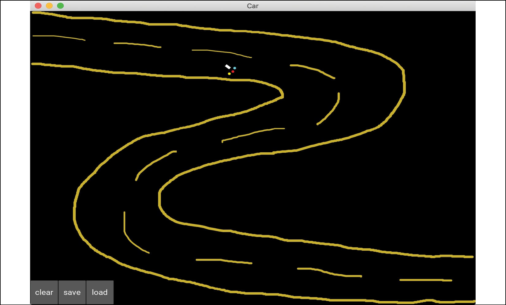
Figure 4: A more challenging road

If you think that road look too easy, here's a more challenging example; this time with not only a more difficult road but also many obstacles:

Figure 5: An even more challenging road

As a final example, I want to share this last map, designed by one of my students, which could belong in the movie Inception:

Figure 6: The most challenging road ever

If you look closely, it's still a path that goes from Airport to Downtown and vice versa, just much more challenging. The AI we create will be able to cope with any of these maps.

I hope you find that as exciting as I do! Keep that level of energy up, because we have quite a lot of work to do.

Setting the parameters

Before you define the input states, the output actions, and the rewards, you must set all of the parameters of the map and the car that will be part of your environment. The inputs, outputs, and rewards are all functions of these parameters. Let's list them all, using the same names as in the code, so that you can easily understand the file map.py:

1. angle: The angle between the x-axis of the map and the axis of the car
2. rotation: The last rotation made by the car (we will see later that when playing an action, the car makes a rotation)
3. pos = (self.car.x, self.car.y): The position of the car (self.car.x is the x-coordinate of the car, self.car.y is the y-coordinate of the car)
4. velocity = (velocity_x, velocity_y): The velocity vector of the car
5. sensor1 = (sensor1_x, sensor1_y): The position of the first sensor
6. sensor2 = (sensor2_x, sensor2_y): The position of the second sensor
7. sensor3 = (sensor3_x, sensor3_y): The position of the third sensor
8. signal1: The signal received by sensor 1
9. signal2: The signal received by sensor 2
10. signal3: The signal received by sensor 3

Now let's slow down; we've got to define how these signals are computed. The signals are a measure of the density of sand around their sensor. How are you going to compute that density? You start by introducing a new variable, called sand, which you initialize as an array that has as many cells as our graphic interface has pixels. Simply put, the sand array is the black map itself and the pixels are the cells of the array. Then, each cell of the sand array will get a 1 if there is sand, and a 0 if there is not.

For example, here the sand array has only 1s in its first few rows, and the rest is all 0s:

Figure 7: The map with only sand in the first rows

I know the border is a little wobbly—like I said, I'm no great artist—and that just means those rows of the sand array would have 1s where the sand is and 0s where there's no sand.

Now that you have this sand array it's very easy to compute the density of sand around each sensor. You surround your sensor by a square of 20 by 20 cells (which the sensor reads from the sand array), then you count the number of ones in these cells, and finally you divide that number by the total number of cells in that square, that is, 20 x 20 = 400 cells.

Since the sand array only contains 1s (where there's sand) and 0s (where there's no sand), we can very easily count the number of 1s by simply summing the cells of the sand array in this 20 by 20 square. That gives us exactly the density of sand around each sensor, and that's what's computed at lines 81, 82, and 83 in the map.py file:

       self.signal1 = int(np.sum(sand[int(self.sensor1_x)-10:int(self.sensor1_x)+10, int(self.sensor1_y)-10:int(self.sensor1_y)+10]))/400.   #81
        self.signal2 = int(np.sum(sand[int(self.sensor2_x)-10:int(self.sensor2_x)+10, int(self.sensor2_y)-10:int(self.sensor2_y)+10]))/400.   #82
        self.signal3 = int(np.sum(sand[int(self.sensor3_x)-10:int(self.sensor3_x)+10, int(self.sensor3_y)-10:int(self.sensor3_y)+10]))/400.   #83

Now that we've covered how the signals are computed, let's continue with the rest of the parameters. The last parameters, which I've highlighted in the list below, are important because they're the last pieces that we need to reveal the final input state vector. Here they are:

1. goal_x: The x-coordinate of the goal (which can either be the Airport or Downtown)
2. goal_y: The y-coordinate of the goal (which can either be the Airport or Downtown)
3. xx = (goal_x - self.car.x): The difference of x-coordinates between the goal and the car
4. yy = (goal_y - self.car.y): The difference of y-coordinates between the goal and the car
5. orientation: The angle that measures the direction of the car with respect to the goal

Let's slow down again for a moment. We need to know how orientation is computed; it's the angle between the axis of the car (the velocity vector from our first list of parameters) and the axis that joins the goal and the center of the car. The goal has the coordinates (goal_x, goal_y) and the center of the car has the coordinates (self.car.x, self.car.y). For example, if the car is heading perfectly toward the goal, then orientation = 0°. If you're curious as to how we can compute the angle between the two axes in Python, here's the code that gets the orientation (lines 126, 127, and 128 in the map.py file):

       xx = goal_x - self.car.x   #126
        yy = goal_y - self.car.y   #127
        orientation = Vector(*self.car.velocity).angle((xx,yy))/180.   #128

Good news—we're finally ready to define the main pillars of the environment. I'm talking, of course, about the input states, the actions, and the rewards.

Before I define them, try to guess what they're going to be. Check out all the preceding parameters again, and remember the goal: making round trips between two locations, the Airport and Downtown, while avoiding any obstacles along the road. The solution's in the next section.

The input states

What do you think the input states are? You might have answered "the position of the car." In that case, the input state would be a vector of two elements, the coordinates of the car: self.car.x and self.car.y.

That's a good start. From the intuition and foundation techniques of deep Q-learning you learned in Chapter 9, Going Pro with Artificial Brains – Deep Q-Learning, you know that when you're doing deep Q-learning, the input state doesn't have to be a single element as in Q-learning. In fact, in deep Q-learning the input state can be a vector of many elements, allowing you to supply many sources of information to your AI to help it predict smart actions to play.

We can do better than just supplying the car position coordinates. They tell us where the self-driving car is located, but there's another parameter that's better, simpler, and more directly related to the goal. I'm talking about the orientation variable. The orientation is a single input that directly tells us if we are pointed in the right direction, toward the goal. If we have that orientation, we don't need the car position coordinates at all to navigate toward the goal; we can just change the orientation by a certain angle to point the car more in the direction of the goal. The actions that the AI performs will be what changes that orientation. We'll discuss those in the next section.

We have the first element of our input state: the orientation.

But that's not enough. Remember that we also have another goal, or, should I say, constraint. Our car needs to stay on the road and avoid any obstacles along that road.

In the input state, we need information telling the AI whether it is about to move off the road or hit an obstacle. Try and work it out for yourself—do we have a way to get this information?

The solution is the sensors. Remember that our car has three sensors giving us signals about how much sand is around them. The blue sensor tells us if there's any sand at the left of the car, the red sensor tells us if there is any sand in front of the car, and the yellow sensor tells us if there is any sand at the right of the car. The signals of these sensors are already coded into three variables: signal1, signal2, and signal3. These signals will tell the AI if it's about to hit some obstacle or about to get out of the road, since the road is delimited by sand.

That's the rest of the information you need for your input state. With these four elements, signal1, signal2, signal3, and orientation, you have everything you need to be able to drive from one location to another, while staying on the road, and without hitting any obstacles.

In conclusion, here's what the input state is going to be at each time:

Input state = (orientation, signal1, signal2, signal3)

And that's exactly what's coded at line 129 in the map.py file:

        state = [orientation, self.car.signal1, self.car.signal2, self.car.signal3]   #129

state is the variable name given to the input state.

We've covered the input state; now let's tackle the actions.

The output actions

I've already briefly mentioned or suggested what the actions are going to be. Given our input state, it's easy to guess. Naturally, since you're building a self-driving car, you might think that the actions should be: move forward, turn left, or turn right. You'd be absolutely right! That's exactly what the actions are going to be.

Not only is this intuitive, but it aligns extremely well with our choice of input states. They contain the orientation variable that tells us if we're aimed in the right direction toward the goal. Simply put, if the orientation input tells us our car is pointed in the right direction, we perform the action of moving forward. If the orientation input tells us that the goal is on the right of our car, we perform the action of turning right. Finally, if the orientation tells us that the goal is on the left of our car, we perform the action of turning left.

At the same time, if any of the signals spot some sand around the car, the car will turn left or right to avoid it. The three possible actions of move forward, turn left, and turn right make logical sense with the goal, constraint, and input states we have, and we can define them as the three following rotations:

rotations = [turn 0° (that is, move forward), turn 20° to the left, turn 20° to the right]

The choice of 20° is quite arbitrary. You could very well choose 10°, 30°, or 40°. I'd avoid more than 40°, because then your car would have twitchy, fidgety movements, and wouldn't look like a smoothly moving car.

However, the actions the ANN outputs will not be 0°, 20°, and -20°; they will be 0, 1 and 2.

actions = [0, 1, 2]

It's always better to use simple categories like those when you're dealing with the output of an artificial neural network. Since 0, 1, and 2 will be the actions the AI returns, how do you think we end up with the rotations?

You'll use a simple mapping, called action2rotation in our code, which maps the actions 0, 1, 2 to the respective rotations of 0°, 20°, -20°. This is exactly what's coded on lines 34 and 131 of the map.py file:

action2rotation = [0,20,-20]   #34

        rotation = action2rotation[action]   #131

Now, let's move on to the rewards. This one's going to be fun, because this is where you decide how you want to reward or punish your car. Try to figure out how by yourself first, and then take a look at the solution in the following section.

The rewards

To define the system of rewards, we have to answer the following questions:

• In which cases do we give the AI a good reward? How good for each case?
• In which cases do we give the AI a bad reward? How bad for each case?

To answer these questions, we must simply remember what the goal and constraints are:

• The goal is to make round trips between the Airport and Downtown.
• The constraints are to stay on the road and avoid obstacles if any. In other words, the constraint is to stay away from the sand.

Hence, based on this goal and constraints, the answers to our preceding questions are:

1. We give the AI a good reward when it gets closer to the destination.
2. We give the AI a bad reward when it gets further away from the destination.
3. We give the AI a bad reward if it's about to drive onto some sand.

That's it! That should work, because these good and bad rewards have a direct effect on the goal and constraints.

To answer the second part of each question, how good and how bad the reward should be for each case, we'll play the tough card; it's often more effective. The tough card consists of punishing the car more when it makes mistakes than we reward it when it does well. In other words, the bad reward is going to be stronger than the good reward.

This works well in reinforcement learning, but that doesn't mean you should do the same with your dog or your kids. When you're dealing with a biological system, the other way around (high good reward and small bad reward) is a much more effective way to train or educate. Just food for thought.

On that note, here are the rewards we'll give in each case:

1. The AI gets a bad reward of -1 if it drives onto some sand. Nasty!
2. The AI gets a bad reward of -0.2 if it moves away from the destination.
3. The AI gets a good reward of 0.1 if it moves closer to the destination.

The reason we attribute the worst reward (-1) to the case when the car drives onto some sand makes sense. Driving onto sand is what we absolutely want to avoid. The sand on the map represents obstacles in real life; in real life, you would train your self-driving car not to hit any obstacle, so as to avoid any accident. To do so, we penalize the AI with a highly bad reward when it does hit an obstacle during its training.

How's that translated that into code? That's easy; you just take your sand array and check if the car has just moved onto a cell that contains a 1. If it does, that means the car has moved onto some sand and must therefore get a bad reward of -1. That's exactly what's coded here at lines 138, 139, and 140 of the map.py file (including an update of the car velocity vector, which not only updates the speed by slowing the car down to 1, but also updates the direction of the car by a certain angle, self.car.angle):

       if sand[int(self.car.x),int(self.car.y)] > 0:   #138
            self.car.velocity = Vector(1, 0).rotate(self.car.angle)   #139
            reward = -1   #140

Then for the other reward attributions, you just have to complete the if condition preceding with an else, which will say what happens in the case where the car has not driven onto some sand.

In that case, you start a new if and else condition, saying that if the car has moved away from the destination, you give it a bad reward of -0.2, and, if the car has moved closer to the destination, you give it a good reward of 0.1. The way you measure if the car is getting away from or closer to the goal is by comparing two distances put into two separate variables: last_distance, which is the previous distance between the car and the destination at time t-1, and distance, which is the current distance between the car and the destination at time t. If you put all that together, you get the following code, which completes the preceding lines of code:

       if sand[int(self.car.x),int(self.car.y)] > 0:   #138
            self.car.velocity = Vector(1, 0).rotate(self.car.angle)   #139
            reward = -1   #140
        else:   #141
            self.car.velocity = Vector(6, 0).rotate(self.car.angle)   #142
            reward = -0.2   #143
            if distance < last_distance:   #144
                reward = 0.1   #145

To keep the car from trying to veer off the map, lines 147 to 158 of the map.py file punish the AI with a bad reward of -1 if the self-driving car gets within 10 pixels of any of the map's 4 borders of the map. Finally, lines 160 to 162 of the map.py file update the goal, switching it from the Airport to Downtown, or vice versa, anytime the car gets within 100 pixels of the current goal.

AI solution refresher

Let's refresh our memory by reminding ourselves of the steps of the deep Q-learning process, while adapting them to our self-driving car application.

Initialization:

1. The memory of the experience replay is initialized to an empty list, called memory in the code.
2. The maximum size of the memory is set, called capacity in the code.

At each time t, the AI repeats the following process, until the end of the epoch:

1. The AI predicts the Q-values of the current state S_t. Therefore, since three actions can be played (0 <-> 0°, 1 <-> 20°, or 2 <-> -20°), it gets three predicted Q-values.
2. The AI performs an action selected by the Softmax method (see Chapter 5, Your First AI Model – Beware the Bandits!):

   

3. The AI receives a reward , which is one of -1, -0.2 or +0.1.
4. The AI reaches the next state , which is composed of the next three signals from the three sensors, plus the orientation of the car.
5. The AI appends the transition to the memory.
6. The AI takes a random batch of transitions. For all the transitions of the random batch B:
   • The AI gets the predictions:
   • The AI gets the targets:
   • The AI computes the loss between the predictions and the targets over the whole batch B:

     

   • Finally, the AI backpropagates this loss error into the neural network, and through stochastic gradient descent updates the weights according to how much they contributed to the loss error.

Implementation

Now it's time for the implementation! The first thing you need is a professional toolkit, because you're not going to build an artificial brain with simple Python libraries. What you need is an advanced framework, which allows fast computation for the training of neural networks.

Today, the best frameworks to build and train AIs are TensorFlow (by Google) and PyTorch (by Facebook). How should you choose between the two? They're both great to work with and equally powerful. They both have dynamic graphs, which allow the fast computation of the gradients of complex functions needed to train the model during backpropagation with mini-batch gradient descent. Really, it doesn't matter which framework you choose; both work very well for our self-driving car. As far as I'm concerned, I have slightly more experience with PyTorch, so I'm going to opt for PyTorch and that's how the example in this chapter will continue to play out.

To take a step back, our self-driving car implementation is composed of three Python files:

1. car.kv, which contains the Kivy objects (rectangle shape of the car and the three sensors)
2. map.py, which builds the environment (map, car, input states, output actions, rewards)
3. deep_q_learning.py, which builds and trains the AI through deep Q-learning

We've already covered the major elements of map.py, and now we're about to tackle deep_q_learning.py, where you'll not only build an artificial neural network, but also implement the deep Q-learning training process. Let's get started!

Step 1 – Importing the libraries

As usual, you start by importing the libraries and modules you need to build your AI. These include:

1. os: The operating system library, used to load the saved AI models.
2. random: Used to sample some random transitions from the memory for experience replay.
3. torch: The main library from PyTorch, which will be used to build our neural network with tensors, as opposed to simple matrices like numpy arrays. While a matrix is a 2-D array, a tensor can be a n-dimensional array, with more than just a single number in its cells. Here's a diagram so you can clearly understand the difference between a matrix and a tensor:

   

4. torch.nn: The nn module from the torch library, used to build the fully connected layers in the artificial neural network of our AI.
5. torch.nn.functional: The functional sub-module from the nn module, used to call the activation functions (rectifier and Softmax), as well as the loss function for backpropagation.
6. torch.optim: The optim module from the torch library, used to call the Adam optimizer, which computes the gradients of the loss with respect to the weights and updates those weights in directions that reduce the loss.
7. torch.autograd: The autograd module from the torch library, used to call the Variable class, which associates each tensor and its gradient into the same variable.

That makes up your first code section:

# AI for Autonomous Vehicles - Build a Self-Driving Car   #1
#2
# Importing the libraries   #3
#4
import os   #5
import random   #6
import torch   #7
import torch.nn as nn   #8
import torch.nn.functional as F   #9
import torch.optim as optim   #10
from torch.autograd import Variable   #11

Step 2 – Creating the architecture of the neural network

This code section is where you really become the architect of the brain in your AI. You're about to build the input layer, the fully connected layers, and the output layer, while choosing some activation functions that will forward-propagate the signal inside the brain.

First, you build this brain inside a class, which we are going to call Network.

What is a class? Let's explain that before we explain why you're using one. A class is an advanced structure in Python that contains the instructions of an object we want to build. Taking the example of your neural network (the object), these instructions include how many layers you want, how many neurons you want inside each layer, which activation function you choose, and so on. These parameters define your artificial brain and are all gathered in what we call the __init__() method, which is what we always start with when building a class. But that's not all—a class can also contain tools, called methods, which are functions that either perform some operations or return something. Your Network class will contain one method, which forward-propagates the signal inside the neural network and returns the predicted Q-values. Call this method forward.

Now, why use a class? That's because building a class allows you to create as many objects (also called instances) as you want, and easily switch from one to another by just changing the arguments of the class. For example, your Network class contains two arguments: input_size (the number of inputs) and nb_actions (the number of actions). If you ever want to build an AI with more inputs (besides the signals and the orientation) or more outputs (you could add an action that brakes the car), you'll do it in a flash thanks to the advanced structure of the class. It's super practical, and if you're not already familiar with classes you'll have to get familiar with them. Nearly all AI implementations are done with classes.

That was just a short technical aside to make sure I don't lose anybody on the way. Now let's build this class. As there are many important elements to explain in the code, and since you're probably new to PyTorch, I'll show you the code first and then explain it line by line from the deep_q_learning.py file:

# Creating the architecture of the Neural Network   #13
#14
class Network(nn.Module):   #15
    #16
    def __init__(self, input_size, nb_action):   #17
        super(Network, self).__init__()   #18
        self.input_size = input_size   #19
        self.nb_action = nb_action   #20
        self.fc1 = nn.Linear(input_size, 30)   #21
        self.fc2 = nn.Linear(30, nb_action)   #22
    #23
    def forward(self, state):   #24
        x = F.relu(self.fc1(state))   #25
        q_values = self.fc2(x)   #26
        return q_values   #27

Line 15: You introduce the Network class. In the parenthesis of this class, you can see nn.Module. That means you're calling the Module class, which is an existing class taken from the nn module, in order to get all the properties and tools of the Module class and use them inside your Network class. This trick of calling another existing class inside a new class is called inheritance.

Line 17: You start with the __init__() method, which defines all the parameters (number of inputs, number of outputs, and so on) of your artificial neural network. You can see three arguments: self, input_size, and nb_action.self refer to the object, that is, to the future instance of the class that will be created after the class is done. Any time you see self before a variable, and separated by a dot (like self.variable), that means the variable belongs to the object. That should clear up any mystery about self!

Then, input_size is the number of inputs in your input state vector (thus 4), and nb_action is the number of output actions (thus 3). What's important to understand is that the arguments (other than self) of the __init__() method are the ones you will enter when creating the future object, which is the future artificial brain of your AI.

Line 18: You use the super() function to activate the inheritance (explained in Line 15), inside the __init__() method.

Line 19: Here you introduce the first object variable, self.input_size, set equal to the argument input_size (which will later be entered as 4, since the input state has 4 elements).

Line 20: You introduce the second object variable, self.nb_action, set equal to the argument nb_action (which will later be entered as 3, since there are three actions that can be performed).

Line 21: You introduce the third object variable, self.fc1, which is the first full connection between the input layer (composed of the input state) and the hidden layer. That first full connection is created as an object of the nn.Linear class, which takes two arguments: the first one is the number of elements in the left layer (the input layer), so input_size is the right argument to use, and the second one is the number of hidden neurons in the right layer (the hidden layer). Here, you choose to have 30 neurons, and therefore the second argument is 30. The choice of 30 is purely arbitrary, and the self-driving car could work well with any other numbers.

Line 22: You introduce the fourth object variable, self.fc2, which is the second full connection between the hidden layer (composed of 30 hidden neurons) and the output layer. It could have been a full connection with a new hidden layer, but your problem is not complex enough to need more than one hidden layer, so you'll just have one hidden layer in your artificial brain. Just like before, that second full connection is created as an object of the nn.Linear class, which takes two arguments: the first one is the number of elements in the left layer (the hidden layer), therefore 30, and the second one is the number of hidden neurons in the right layer (the output layer), therefore 3.

Line 24: You start building the first and only method of the class, the forward method, which will propagate the signal from the input layer to the output layer, after which it will return the predicted Q-values. This forward method takes two arguments: self, because you'll use the object variables inside the forward method, and state, the input state vector composed of four elements (orientation plus the three signals).

Line 25: You forward propagate the signal from the input layer to the hidden layer while activating the signal with a rectifier activation function, also called ReLU (Rectified Linear Unit). You do this in two steps. First, the forward propagation from the input layer to the hidden layer is done by calling the first full connection self.fc1 with the input state vector state as input: self.fc1(state).

That returns the hidden layer. And then we call the relu function with that hidden layer as input to break the linearity of the signal the following way:

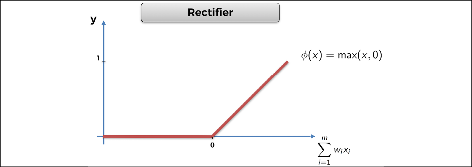
Figure 8: The Rectifier activation function

The purpose of the ReLU layer is to break linearity by creating non-linear operations along the fully connected layers. You'll want to have that, because you're trying to solve a nonlinear problem. Finally, F.relu(self.fc1(state)) returns x, the hidden layer with a nonlinear signal.

Line 26: You forward-propagate the signal from the hidden layer to the output layer containing the Q-values. In the same way as the previous line, this is done by calling the second full connection self.fc2 with the hidden layer x as input: self.fc2(x). That returns the Q-values, which you name q_values. Here, no activation function is needed because you'll select the action to play with Softmax, later, in another class.

Line 27: Finally, here, the forward method returns the Q-values.

Let's have a look at what you've just created!

Figure 9: The neural network (the brain) of our AI

self.fc1 are all the blue connection lines between the Input Layer and the Hidden Layer.

self.fc2 are all the blue connection lines between the Hidden Layer and the Output Layer.

That should help you visualize the full connections better. Great job!

Step 3 – Implementing experience replay

Time for the next step! You'll now build another class, which builds the memory object for experience replay (as seen in Chapter 5, Your First AI Model – Beware the Bandits!). Call this class ReplayMemory. Let's have a look at the code first and then I'll explain everything line by line from the deep_q_learning.py file.

# Implementing Experience Replay   #29
#30
class ReplayMemory(object):   #31
    #32
    def __init__(self, capacity):   #33
        self.capacity = capacity   #34
        self.memory = []   #35
    #36
    def push(self, event):   #37
        self.memory.append(event)   #38
        if len(self.memory) > self.capacity:   #39
            del self.memory[0]   #40
    #41
    def sample(self, batch_size):   #42
        samples = zip(*random.sample(self.memory, batch_size))   #43
        return map(lambda x: Variable(torch.cat(x, 0)), samples)   #44

Line 31: You introduce the ReplayMemory class. This time you don't need to inherit from any other class, so just input object in the parenthesis of the class.

Line 33: As always, you start with the __init__() method, which only takes two arguments: self, the object, and capacity, the maximum size of the memory.

Line 34: You introduce the first object variable, self.capacity, set equal to the argument capacity, which will be entered later when creating an object of the class.

Line 35: You introduce the second object variable, self.memory, initialized as an empty list.

Line 37: You start building the first tool of the class, the push method, which takes a transition as input and adds it to the memory. However, if adding that transition exceeds the memory's capacity, the push method also deletes the first element of the memory. The event argument you can see is the transition to be added.

Line 38: Using the append function, you add the transition to the memory.

Line 39: You start an if condition that checks if the length of the memory (meaning its number of transitions) is larger than the capacity.

Line 40: If that is indeed the case, you delete the first element of the memory.

Line 42: You start building the second tool of the class, the sample method, which samples some random transitions from the experience replay memory. It takes batch_size as input, which is the size of the batches of transitions with which you'll train your neural network.

Remember how it works: instead of forward-propagating single input states into the neural network and updating the weights after each transition resulting from the input state, you forward-propagate small batches of input states and update the weights after backpropagating the same whole batches of transitions with mini-batch gradient descent. That's different from stochastic gradient descent (weight update every single input) and batch gradient descent (weight update every batch of inputs) as explained in Chapter 9, Going Pro with Artificial Brains – Deep Q-Learning:

Figure 10: Batch gradient descent versus stochastic gradient descent

Line 43: You sample some random transitions from the memory and put them into a batch of size batch_size. For example, if batch_size = 100, you sample 100 random transitions from the memory. The sampling is done with the sample() function from the random library. Then, zip(*list) is used to regroup the states, actions, and rewards into separate batches of the same size (batch_size), in order to put the sampled transitions into the format expected by PyTorch (the Variable format, which comes next in Line 44).

This is probably a good time to take a step back. Let's see what Line 43 gives you:

Figure 11: The batches of last states, actions, rewards, and next states

Line 44: Using the map() function, wrap each sample into a torch Variable object (as Variable() is actually a class), so that each tensor inside the samples is associated to a gradient. Simply put, you can see a torch Variable as an advanced structure that encompasses a tensor and a gradient.

This is the beauty of PyTorch. These torch Variables are all in a dynamic graph which allows fast computation of the gradient of complex functions. Those fast computations are required for the weight updates happening during backpropagation with mini-batch gradient descent. Inside the Variable class we see torch.cat(x,0). That's just a concatenation trick, along the vertical axis, to put the samples in the format expected by the Variable class.

The most important thing to remember is this: when training a neural network with PyTorch, we always work with torch Variables, as opposed to just tensors. You can find more details about this in the PyTorch documentation.

Step 4 – Implementing deep Q-learning

You've made it! You're finally about to start coding the whole deep Q-learning process. Again, you'll wrap all of it into a class, this time called Dqn, as in deep Q-network. This is your final run before the finish line. Let's smash this.

This time, the class is quite long so I'll show and explain the lines of code method by method from the deep_q_learning.py file. Here's the first one, the __init__() method:

# Implementing Deep Q-Learning   #46
#47
class Dqn(object):   #48
    #49
    def __init__(self, input_size, nb_action, gamma):   #50
        self.gamma = gamma   #51
        self.model = Network(input_size, nb_action)   #52
        self.memory = ReplayMemory(capacity = 100000)   #53
        self.optimizer = optim.Adam(params = self.model.parameters())   #54
        self.last_state = torch.Tensor(input_size).unsqueeze(0)   #55
        self.last_action = 0   #56
        self.last_reward = 0   #57

Line 48: You introduce the Dqn class. You don't need to inherit from any other class so just input object in the parenthesis of the class.

Line 50: As always, you start with the __init__() method, which this time takes four arguments:

1. self: The object
2. input_size: The number of inputs in the input state vector (that is, 4)
3. nb_action: The number of actions (that is, 3)
4. gamma: The discount factor in the temporal difference formula

Line 51: You introduce the first object variable, self.gamma, set equal to the argument gamma (which will be entered later when you create an object of the Dqn class).

Line 52: You introduce the second object variable, self.model, an object of the Network class you built before. This object is your neural network; in other words, the brain of our AI. When creating this object, you input the two arguments of the __init__() method in the Network class, which are input_size and nb_action. You'll enter their real values (respectively 4 and 3) later, when creating an object of the Dqn class.

Line 53: You introduce the third object variable, self.memory, as an object of the ReplayMemory class you built before. This object is the experience replay memory. Since the __init__ method of the ReplayMemory class only expects one argument, the capacity, that's exactly what you input here as 100,000. In other words, you're creating a memory of size 100,000, which means that instead of remembering just the last transition, the AI will remember the last 100,000 transitions.

Line 54: You introduce the fourth object variable, self.optimizer, as an object of the Adam class, which is an existing class built in the torch.optim module. This object is the optimizer, which updates the weights through mini-batch gradient descent during backpropagation. In the arguments, keep most of the default parameter values (you can check them in the PyTorch documentation) and only enter the model parameters (the params argument), which you access with self.model.parameters, one of the attributes of the nn.Module class from which the Network class inherits.

Line 55: You introduce the fifth object variable, self.last_state, which will be the last state in each (last state, action, reward, next state) transition. This last state is initialized as an object of the Tensor class from the torch library, into which you only have to enter the input_size argument. Then .unsqueeze(0) is used to create an additional dimension at index 0, which will correspond to the batch. This allows us to do something like this, matching each last state to the appropriate batch:

Figure 12: Adding a dimension for the batch

Line 56: You introduce the sixth object variable, self.last_action, initialized as 0, which is the last action played at each iteration.

Line 57: We introduce the last object variable, self.last_reward, initialized as 0, which is the last reward received after playing the last action self.last_action, in the last state self.last_state.

Now, you're all good for the __init__ method. Let's move on to the next code section with the next method: the select_action method, which selects the action to play at each iteration using Softmax.

   def select_action(self, state):   #59
        probs = F.softmax(self.model(Variable(state))*100)   #60
        action = probs.multinomial(len(probs))   #61
        return action.data[0,0]   #62

Line 59: You start defining the select_action method, which takes as input an input state vector (orientation, signal 1, signal 2, signal 3), and returns as output the selected action to play.

Line 60: You get the probabilities of the three actions thanks to the Softmax function taken from the torch.nn.functional module. This Softmax function takes the Q-values as input, which are exactly returned by self.model(Variable(state)). Remember, self.model is an object of the Network class, which has the forward method, which takes as input an input state tensor wrapped into a torch Variable, and returns as output the Q-values for the three actions.

Multiplying the Q-values by a number (here 100) inside softmax is a good trick to remember: it allows you to regulate the Exploration versus Exploitation. The lower that number is, the more you'll explore, and therefore the longer it will take to get optimized actions. Here, the problem's not too complex, so choose a large number (100) in order to have confident actions and a smooth trajectory to the goal. You'll clearly see the difference if you remove *100 from the code. Simply put, with the *100, you'll see a car sure of itself; without the *100, you'll see a car fidgeting.

Line 61: You take a random draw from the distribution of actions created by the softmax function at line 60, by calling the multinomial() function from your probabilities probs.

Line 62: You return the selected action to perform, which you access in action.data[0,0]. The returned action has an advanced tensor structure, and the action index (0, 1, or 2) that you're interested in is located in the data attribute of the action tensor at the first cell of indexes [0,0].

Let's move on to the next code section, the learn method. This one is pretty interesting because it's where the heart of deep Q-learning beats. It's in this method that we compute the temporal difference, and accordingly the loss, and update the weights with our optimizer in order to reduce that loss. That's why this method is called learn, because it is here that the AI learns to perform better and better actions that increase the accumulated reward. Let's continue:

   def learn(self, batch_states, batch_actions, batch_rewards, batch_next_states):   #64
        batch_outputs = self.model(batch_states).gather(1, batch_actions.unsqueeze(1)).squeeze(1)   #65
        batch_next_outputs = self.model(batch_next_states).detach().max(1)[0]   #66
        batch_targets = batch_rewards + self.gamma * batch_next_outputs   #67
        td_loss = F.smooth_l1_loss(batch_outputs, batch_targets)   #68
        self.optimizer.zero_grad()   #69
        td_loss.backward()   #70
        self.optimizer.step()   #71

Line 64: You start by defining the learn() method, which takes as inputs the batches of the four elements composing a transition (input state, action, reward, next state):

1. batch_states: A batch of input states.
2. batch_actions: A batch of actions played.
3. batch_rewards: A batch of the rewards received.
4. batch_next_states: A batch of the next states reached.

Before I explain Lines 65, 66, and 67, let's take a step back and see what you'll have to do. As you know, the goal of this learn method is to update the weights in directions that reduce the back-propagated loss at each iteration of the training. First let's remind ourselves of the formula for the loss:

Inside the formula for the loss, we clearly recognize the outputs (predicted Q-values) and the targets:

Therefore, to compute the loss, you proceed this way over the next four lines of code:

Line 65: You collect the batch of outputs, .

Line 66: You compute the part of the targets, which you call batch_next_outputs.

Line 67: You get the batch of targets.

Line 68: Since you have the outputs and targets, you're ready to get the loss.

Now let's do this in detail.

Line 65: You collect the batch of outputs , meaning the predicted Q-values of the input states and the actions played in the batch. Getting them takes several steps. First, you call self.model(batch_states), which, as seen in Line 60, returns the Q-values of each input state in batch_states and for all the three actions 0, 1, and 2. To help you visualize it better, it returns something like this:

Figure 13: What is returned by self.model(batch_states)

You only want the predicted Q-values for the selected actions from the batch of outputs, which are found in the batch of actions batch_actions. That's exactly what the .gather(1, batch_actions.unsqueeze(1)).squeeze(1) trick does: for each input state of the batch, it picks the Q-value that corresponds to the action that was selected in the batch of actions. To help visualize this better, let's suppose the batch of actions is the following:

Figure 14: Batch of actions

Then you would get the following batch of outputs composed of the red Q-values:

Figure 15: Batch of outputs

I hope this is clear; I'm doing my best not to lose you along the way.

Line 66: Now you get the part of the target. Call this batch_next_outputs; you get it in two steps. First, call self.model(batch_next_states) to get the predicted Q-values for each next state of the batch of next states and for each of the three actions. Then, for each next state of the batch, take the maximum of the three Q-values using .detach().max(1)[0]. That gives you the batch of the values part of the targets.

Line 67: Since you have the batch of rewards (it's part of the arguments), and since you just got the batch of the values part of the targets at Line 66, then you're ready to get the batch of targets:

That's exactly what you do at Line 67, by summing batch_rewards and batch_next_outputs multiplied by self.gamma, one of the object variables in the Dqn class. Now you have both the batch of outputs and the batch of targets, so you're ready to get the loss.

Line 68: Let's remind ourselves of the formula for the loss:

Therefore, in order to get the loss, you just have to get the sum of the squared differences between our targets and outputs in the batch. That's exactly what the smooth_l1_loss function will do. Taken from the torch.nn.functional module, it takes as inputs the two batches of outputs and targets and returns the loss as given in the preceding formula. In the code, call this loss td_loss as in temporal difference loss.

Excellent progress! Now that you have the loss, representing the error between the predictions and the targets, you're ready to backpropagate this loss into the neural network and update our weights to reduce this loss through mini-batch gradient descent. That's why the next step to take here is to use your optimizer, which is the tool that will perform the updates to the weights.

Line 69: You first initialize the gradients, by calling the zero_grad() method from your self.optimizer object (zero_grad is a method of the Adam class), which will basically set all the gradients of the weights to zero.

Line 70: You backpropagate the loss error td_loss into the neural network by calling the backward() function from td_loss.

Line 71: You perform the weights updates by calling the step() method from your self.optimizer object (step is a method of the Adam class).

Congratulations! You've built yourself a tool in the Dqn class that will train your car to drive better. You've done the toughest part. Now all you have left to do is to wrap things up into a last method, called update, which will simply update the weights after reaching a new state.

Now, in case you are thinking, "but isn't what I've already done with the learn method?," well, you're right; but you need to make an extra function that will update the weights at the right time. The right time to update the weights is right after our AI reaches a new state. Simply put, this final update method you're about to implement will connect the dots between the learn method and the dynamic environment.

That's the finish line! Are you ready? Here's the code:

   def update(self, new_state, new_reward):   #73
        new_state = torch.Tensor(new_state).float().unsqueeze(0)   #74
        self.memory.push((self.last_state, torch.LongTensor([int(self.last_action)]), torch.Tensor([self.last_reward]), new_state))   #75
        new_action = self.select_action(new_state)   #76
        if len(self.memory.memory) > 100:   #77
            batch_states, batch_actions, batch_rewards, batch_next_states = self.memory.sample(100)   #78
            self.learn(batch_states, batch_actions, batch_rewards, batch_next_states)   #79
        self.last_state = new_state   #80
        self.last_action = new_action   #81
        self.last_reward = new_reward   #82
        return new_action   #83

Line 73: You introduce the update() method, which takes as input the new state reached and the new reward received right after playing an action. This new state entered here will be the state variable you can see in Line 129 of the map.py file and this new reward will be the reward variable you can see in Lines 138 to 145 of the map.py file. This update method performs some operations including the weights updates and, in the end, returns the new action to perform.

Line 74: You first convert the new state into a torch tensor and unsqueeze it to create an additional dimension (placed first in index 0) corresponding to the batch. To ease future operations, you also make sure that all the elements of the new state (orientation plus the three signals) are converted into floats by adding .float().

Line 75: Using the push() method from your memory object, add a new transition to the memory. This new transition is composed of:

1. self.last_state: The last state reached before reaching that new state
2. self.last_action: The last action played that led to that new state
3. self.last_reward: The last reward received after performing that last action
4. new_state: The new state that was just reached

All the elements of this new transition are converted into torch tensors.

Line 76: Using the select_action() method from your Dqn class, perform a new action from the new state just reached.

Line 77: Check if the size of the memory is larger than 100. In self.memory.memory, the first memory is the object created at Line 53 and the second memory is the variable object introduced at Line 35.

Line 78: If that's the case, sample 100 transitions from the memory, using the sample() method from your self.memory object. This returns four batches of size 100:

1. batch_states: The batch of current states (current at the time of the transition).
2. batch_actions: The batch of actions performed in the current states.
3. batch_rewards: The batch of rewards received after playing the actions of batch_actions in the current states of batch_states.
4. batch_next_states: The batch of next states reached after playing the actions of batch_actions in the current states of batch_states.

Line 79: Still in the if condition, proceed to the weights updates using the learn() method called from the same Dqn class, with the four previous batches as inputs.

Line 80: Update the last state reached, self.last_state, which becomes new_state.

Line 81: Update the last action performed, self.last_action, which becomes new_action.

Line 82: Update the last reward received, self.last_reward, which becomes new_reward.

Line 83: Return the new action performed.

That's it for the update() method! I hope you can see how we connected the dots. Now, to connect the dots even better, let's see where and how you call that update method in the map.py file.

First, before calling that update() method, you have to create an object of the Dqn class, which here is called brain. That's exactly what you do in Line 33 of the map.py file.

brain = Dqn(4,3,0.9)   #33

The arguments entered here are the three arguments we see in the __init__() method of the Dqn class:

• 4 is the number of elements in the input state (input_size).
• 3 is the number of possible actions (nb_action).
• 0.9 is the discount factor (gamma).

Then, from this brain object, you call on the update() method in Line 130 of the map.py file, right after reaching a new state, called state in the code:

       state = [orientation, self.car.signal1, self.car.signal2, self.car.signal3]   #129
        action = brain.update(state, reward)   #130

Going back to your Dqn class, you need two extra methods:

1. The save() method, which saves the weights of the AI's network after their last updates. This method will be called as soon as you click the save button while running the map. The weights of your AI will be then saved and put into a file named last_brain.pth, which will automatically be populated in the folder that contains your Python files. That's what allows you to have a pre-trained AI.
2. The load() method, which loads the saved weights in the last_brain.pth file. This method will be called as soon as you click the load button while running the map. It allows you to start the map with a pre-trained self-driving car, without having to wait for it to train.

These last two methods aren't AI-related, so we won't spend time explaining each line of their code. Still, it's good for you to be able to recognize these two tools in case you want to use them for another AI model that you build with PyTorch.

Here's how they're implemented:

    def save(self):   #85
        torch.save({'state_dict': self.model.state_dict(),   #86
                    'optimizer' : self.optimizer.state_dict(),   #87
                   }, 'last_brain.pth')   #88
    #89
    def load(self):   #90
        if os.path.isfile('last_brain.pth'):   #91
            print("=> loading checkpoint... ")   #92
            checkpoint = torch.load('last_brain.pth')   #93
            self.model.load_state_dict(checkpoint['state_dict'])   #94
            self.optimizer.load_state_dict(checkpoint['optimizer'])   #95
            print("done !")   #96
        else:   #97
            print("no checkpoint found...")   #98

Congratulations!

That's right! You've finished this 100 lines of code implementation of the AI inside our self-driving car. That's quite an accomplishment, especially when coding deep Q-learning for the first time. You really can be proud to have gone this far.

After all this hard work, you definitely deserve to have some fun, and I think it'll be the most fun to watch the result of your hard work. In other words, you're about to see your self-driving car in action! I remember I was so excited the first time I ran this. You'll feel it too; it's pretty cool!

The demo

I have some good news and some bad news.

I'll start with the bad news: we can't run the map.py file with a simple plug and play on Google Colab. The reason for that is that Kivy is very tricky to install through Colab. So, we'll go for the classic method of running a Python file: through the terminal.

The good news is that once we install Kivy and PyTorch through the terminal, you'll have a fantastic demo!

Let's install everything we need to run our self-driving car. Here's what we have to install, in the following order:

1. Anaconda: A free and open source distribution of Python that offers an easy way to install packages thanks to the conda command. This is what we'll use to install PyTorch and Kivy.
2. Virtual environment with Python 3.6: Anaconda is installed with Python 3.7 or higher; however, that 3.7 version is not compatible with Kivy. We'll create a virtual environment in which we install Python 3.6, a version compatible with both Kivy and our implementation. Don't worry if that sounds intimidating, I'll give you all the details you need to set this up.
3. PyTorch: Then, inside the virtual environment, we'll install PyTorch, the AI framework used to build our deep Q-network. We'll install a specific version of PyTorch that's compatible with our implementation, so that everyone can be on the same page and run it with no issues. PyTorch upgrades sometimes include changes in the names of the modules, which can make an old implementation incompatible with the newest PyTorch versions. Here, we know we have the right PyTorch version for our implementation.
4. Kivy: To finish, still inside the virtual environment, we'll install Kivy, the open source Python framework on which we will run our map.

Let's start with Anaconda.

Installing Anaconda

On Google, or your favorite browser, go to www.anaconda.com. On the Anaconda website, click Download on the upper right corner of the screen. Scroll down and you'll find the Python versions to download:

Figure 16: Installing Anaconda – Step 2

At the top, make sure that your system (Windows, macOS, or Linux) is correctly selected. If it is, click the Download button in the Python 3.7 version box. This will download Anaconda with Python 3.7.

Then double-click the downloaded file and keep clicking Continue and Agree to install, until the end. If you're prompted to choose who or how to install it for, choose install for me only.

Creating a virtual environment with Python 3.6

Now that Anaconda's installed, you can create a virtual environment, named selfdrivingcar, with Python 3.6 installed. To do this you need to open a terminal and enter some commands. Here's how to open it for the three systems:

1. For Linux users, just pressCtrl + Alt + T.
2. For Mac users, press Cmd + Space, and then in the Spotlight Search enter Terminal.
3. For Windows users, click the Windows button at the lower left corner of your screen, find anaconda in the list of programs, and click to open Anaconda prompt. A black window will open; that's the terminal you'll use to install the packages.

Inside the terminal, enter the following command:

conda create -n selfdrivingcar python=3.6

Just like so:

This command creates a virtual environment called selfdrivingcar with Python 3.6 and other packages installed.

After pressing Enter, you'll get this in a few seconds:

Press y to proceed. This will download and extract the packages. After a few seconds, you'll get this, which marks the end of the installation:

Then we're going to activate the selfdrivingcar virtual environment, meaning we're going to get inside it in order to install PyTorch and Kivy within the selfdrivingcar virtual environment.

As you can see just preceding, to activate the environment, we will enter the following command:

conda activate selfdrivingcar

Enter that command, and then you'll get inside the virtual environment:

Now we can see (selfdrivingcar) before my computer's name, hadelins-macbook-pro, which means we are inside the selfdrivingcar virtual environment.

We're ready for the next steps, which are the installation of PyTorch and Kivy inside this virtual environment. Don't close your terminal, or when you open it again you'll be back in the main environment.

Installing PyTorch

Now we're going to install PyTorch inside the virtual environment by entering the following command:

conda install pytorch==0.3.1 -c pytorch

Just like so:

After a few seconds, we get this:

Press y again, and then press Enter.

After a few seconds, PyTorch is installed:

Installing Kivy

Now let's proceed to Kivy. In the same virtual environment, we're going to install Kivy by entering the following command:

conda install -c conda-forge/label/cf201901 kivy

Again, we get this:

Enter y again, and after a few seconds more, Kivy is installed.

Now I have some terrific news for you: you're ready to run the self-driving car! To do that, we need to run our code in the terminal, still inside our virtual environment.

So, let's run the code! If you haven't already, download the whole repository by clicking the Clone or download button on the GitHub page:

(https://github.com/PacktPublishing/AI-Crash-Course)

Figure 17: The GitHub repository

Then unzip it and move the unzipped folder to your desktop, just like so:

Now go into Chapter 10 and select and copy all the files inside:

Then, because we're only interested in these files right now, and to simplify the command lines in the terminal, paste these files inside the main AI-Crash-Course-master folder and remove all the rest, which we don't need, so that you eventually end up with this:

Now we're going to access this folder from the terminal. Since we put the repository folder in the desktop, we will find it in a flash. Back into the terminal, enter ls (l as in lion) to see in which folder you are in your machine:

I can see that I'm in my main root folder, which contains the Desktop folder. It should usually be the case for you too. So now we're going to go into the Desktop folder by entering the following command:

cd Desktop

Enter ls again and check that you indeed see the AI-Crash-Course-master folder:

Then go into the AI-Crash-Course-master folder by entering the following command:

cd AI-Crash-Course-master

Perfect! Now we're in the right spot! By entering ls again, you can see all the files of the repo, including the map.py file, which is the one we have to run to see our self-driving car in action!

If by any chance you had trouble getting to this point, that may be because your main root folder doesn't contain your Desktop folder. If that's the case, just put the AI-Crash-Course-master repo folder inside one of the folders that you see when entering the ls command in the terminal, and redo the same process.

What you have to do is just find and enter the AI-Crash-Course-master folder with the cd commands. That's it! Don't forget to make sure your AI-Crash-Course-master folder only contains the self-driving car files:

Now you're only one command line away from running your self-driving car. I hope you're excited to see the results of your hard work; I know exactly how you feel, I was in your shoes not so long ago!

So, without further ado, let's enter the final command, right now. It's this:

python map.py

As soon as you enter it, the map with the car will pop up just like so:

Figure 18: The map

For the first minute or so, your self-driving car will explore its actions by performing nonsense movements; you might see it spinning around. After each 100 movements, the weights inside the neural network of the AI get updated, and the car improves its actions to get higher rewards. And suddenly, maybe after another 30 seconds or so, you should see your car making round trips between the Airport and Downtown, which I highlighted here again:

Figure 19: The destinations

Now have some fun! Draw some obstacles on the map to see if the car avoids them.

On my side I have just drawn this, and after a few more minutes of training, I can clearly see the car avoiding the obstacles:

Figure 20: Road with obstacles

And you can have even more fun! By, for example, drawing a road like so:

Figure 21: The road of the demo

After a few minutes of training, the car becomes able to self-drive along that road, while making many road trips between the Airport and Downtown.

Quick question for you: how did you program the car to travel between the destinations?

You did it by giving a small positive reward to the AI when the car gets closer to the goal. That's programmed in rows 144 and 145 inside the map.py file:

           if distance < last_distance:   #144
                reward = 0.1   #145

Congratulations to you for completing this massive chapter on this not-so-basic self-driving car application! I hope you had fun, and that you feel proud to have mastered such an advanced model in deep reinforcement learning.

Summary

In this chapter, we learned how to build a deep Q-learning model to drive a self-driving car. As inputs it took the information from the three sensors and its current orientation. As outputs it decided the Q-values for each of the actions of going straight, turning left, or turning right. As for the rewards, we punished it badly for hitting the sand, punished it slightly for going in the wrong direction, and rewarded it slightly for going in the right direction. We made the AI implementation in PyTorch and used Kivy for the graphics. To run all of this we used the Anaconda environment.

Now take a long break, you deserve it! I'll see you in the next chapter for our next AI challenge, where this time we will solve a real-world business problem with cost implications running into the millions.