6

Engineering Distributed Training

In the previous chapter, we discussed how to select optimal hardware for the Deep Learning (DL) training job and optimize your model for the target hardware platform. In this chapter, we will consider, in depth, how to design efficient distributed training on Amazon SageMaker given your particular use case and model architecture.

There are two specific problems that distributed training aims to address. The first problem is how to reduce the training time of large models by distributing training tasks across multiple compute devices. Another problem arises when we need to train large models that cannot fit into the memory of a single GPU device. This problem is especially relevant for NLP tasks where it’s shown that very large models have more expressive power and, hence, better performance on a wide range of NLP tasks. For instance, the latest open source SOTA language model, called BLOOM, was trained for ~3.5 months on a compute cluster with 384 GPU accelerators (NVIDIA A100). Model weights alone are around 329 GB, and a checkpoint with model weights and optimizer states is 2.3 TB. For more details, please refer to the model card at https://huggingface.co/bigscience/bloom.

Two approaches have emerged to address these problems; the first is Data parallel distributed training to speed up training time by simultaneously distributing tasks. The second is Model parallel distributed training to distribute large models between several GPUs and, hence, allow you to use models that cannot fit into the memory of an individual GPU device.

As you probably already guessed, large models that do not fit a single GPU device also require considerable time to train. So, inevitably, model parallelism will need to be combined with data parallelism to make the training time acceptable. The combination of data parallelism and model parallelism is known as hybrid parallelism. In this chapter, we will discuss these three types of parallelism.

While understanding distributed training approaches is essential, you also need to understand the available implementations for your DL framework and model architecture. SageMaker provides proprietary libraries for distributed training: SageMaker Distributed Data Parallel (SDDP) and SageMaker Distributed Model Parallel (SDMP). We will review their benefits and gain practical experience in how to use them in this chapter. Additionally, we will discuss other popular open source alternatives for distributed training for both the TensorFlow and PyTorch frameworks and how to use them on the SageMaker platform.

In this chapter, we will cover the following topics:

• Engineering data parallel training
• Engineering model parallel and hybrid training
• Optimizing distributed training jobs

By the end of this chapter, you will have a good understanding of distributed training and will have gained practical experience of how to implement various types of distributed training on Amazon SageMaker.

Technical requirements

In this chapter, we will provide code walk-through samples, so you can develop practical skills. The full code examples are available at https://github.com/PacktPublishing/Accelerate-Deep-Learning-Workloads-with-Amazon-SageMaker/blob/main/chapter6/.

To follow along with this code, you will need to have the following:

• An AWS account and IAM user with the permissions to manage Amazon SageMaker resources.
• A SageMaker Notebook, SageMaker Studio Notebook, or local SageMaker-compatible environment established.
• Access to GPU training instances in your AWS account. Each example in this chapter will provide a recommended instance type to use. It’s possible that you will need to increase your compute quota for SageMaker Training Job to have GPU instances enabled. In that case, please follow the instructions at https://docs.aws.amazon.com/sagemaker/latest/dg/regions-quotas.html.

Engineering data parallel training

First, let’s outline some important terminology that we’ll use throughout this chapter:

• Training process, trainer, or worker – These terms are used interchangeably to identify an independent training process in a compute cluster. For example, a distributed DL training process usually runs on a single GPU device.
• Training node, server, or host – These terms define the server in the training cluster. The server can have one or several GPU devices, which means that one or several training processes can run on the same server.
• World size – This is the number of independent training processes running in the training cluster. Typically, the world size is equal to the number of GPU devices that are available in your training cluster.
• Rank (also global rank) – This is a unique zero-based ID of training processes running in your training cluster. For instance, if you have 4 training processes, they will have the ranks of 0, 1, 2, and 3.
• Local rank – This is a unique zero-based ID of training processes running within a single node. For example, if you have two training nodes with two GPU devices each, then the local ranks will be 0 and 1, and the global ranks will be 0, 1, 2, and 3.
• Communication backend or Collective communication – These terms define the mechanism and protocol for training processes to communicate and coordinate computations with each other. Some popular backends are NVIDIA NCCL, Gloo, and Message passing interface (MPI).
• Collective operation – This is a specific operation performed between the processes of a training cluster, such as the allreduce operation, to aggregate and average tensors or broadcast to send the tensor from one training process to other processes in your cluster. Typically, communication backends provide the implementation of collective operations.

Now that we understand the basic terminology of distributed training, let’s review data parallelism in depth.

Data parallel distributed training is useful when you are looking to reduce the training time of your model across multiple training devices. Each individual training process has a copy of the global model but trains it on a unique slice of data in parallel with others (hence data parallelism). At the end of the training step, each training process exchanges with other learned gradient updates. Then, the gradient updates are averaged and distributed back to all training processes so that they can update their individual model copies. Figure 6.1 illustrates how data batches are distributed in a data-parallel two-node two-GPU cluster:

Figure 6.1 – An overview of data parallelism

When engineering your data parallel training job, you need to be aware of several key design choices to debug and optimize your training job, such as the following:

• How the coordination happens between processes
• How individual compute processes communicate with each other
• How compute processes are distributed in the training cluster

In the following section, we will discuss these design options.

Coordination patterns – Parameter Server versus Allreduce

There are two ways to coordinate compute processes in distributed clusters: using a dedicated centralized coordinator and using peer-to-peer coordination where each node communicates with one or many peers in a cluster directly. In the context of data parallel training, a centralized coordination pattern is called Parameter Server where the parameter server process coordinates the distribution of gradient updates and maintains a global model copy. The peer-to-peer pattern is called Allreduce that goes by the name of the peer-to-peer algorithm to distribute gradient updates between the training processes. In Figure 6.2, you can see the difference between the two coordination patterns:

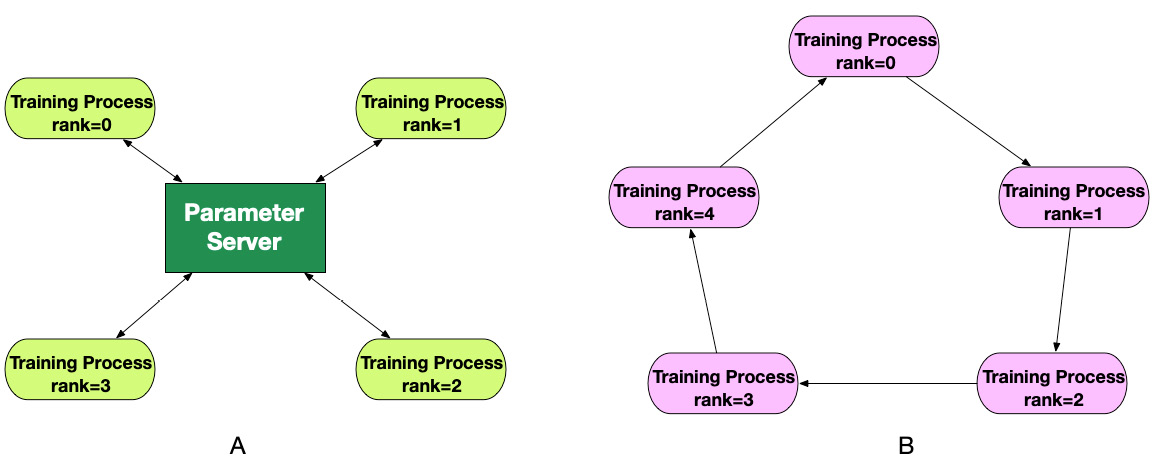
Figure 6.2 – The Parameter Server (A) and Allreduce (B) coordination patterns

Parameter Server is responsible for coordinating training processes in the cluster, namely the following:

• Allocating a unique set of data records for each training process
• Receiving gradients from each individual training process
• Aggregating gradients and updating the model weights accordingly
• Sending the updated model back to the training processes

Parameter Server stores a master copy of model weights. For larger DL models, it’s possible that you might not be able to store the full model on Parameter Server. Additionally, Parameter Server can become a network and computation bottleneck. In that case, you might introduce multiple parameter servers that will store a subset of model parameters to reduce the network and memory requirements. Multiple parameter servers allow you to scale your distributed training for large models; however, it introduces additional complexities when coordinating model updates between the training processes and parameter servers and might still lead to network congestion. Finding an optimal configuration between the training processes and parameter servers can be a daunting task with a considerable trial-and-error effort required to find the optimal configuration.

The Allreduce algorithm employs peer-to-peer communication when each training process exchanges gradient updates with only two neighbors. A training process with a rank of i calculates gradients for the unique data micro-batch, receives gradients from process i-1, summarizes the received gradients with its own calculated gradients, and then sends the aggregated gradients to node i+1. In total, each process will communicate with its peers times:

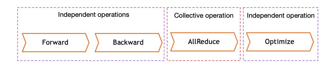
Figure 6.3 – The sequence of compute operations in the Allreduce algorithm

The Allreduce algorithm is considered bandwidth-efficient with constant communication costs and avoids having communication bottlenecks such as in the case of Parameter Server. Additionally, it has less complexity in operating compared to the Parameter Server approach (specifically, in the case of multiple parameter server instances). Therefore, many recent research papers and implementations are based on the Allreduce algorithm and its modifications. The most popular implementations of the Allreduce algorithm are Horovod, TensorFlow Mirror Strategy, and PyTorch Distributed Data Parallel (DDP). AWS utilizes the modified Allreduce algorithm in the SDDP library, too. Later in this chapter, we will develop a distributed training job on SageMaker using the previously mentioned Allreduce implementations.

Communication types – sync versus async

There are two types of communication in distributed training jobs: synchronous (sync) and asynchronous (async).

Sync communication implies that each training process will perform its computations synchronously with other processes in the cluster. For instance, in the case of the synchronous Allreduce algorithm, each training process will wait for other processes to complete their backward and forward passes before starting to exchange their gradients. This leads to situations where the cluster performance on each training step is defined by the performance of the slowest training process and might result in waiting for time (waste) for other training processes. However, the benefits of sync communication include more stable training convergence. Different implementations of the Allreduce algorithm also provide optimizations to reduce waiting time.

In async communication, each node acts independently. It sends gradient updates to other processes or centralized parameter servers and proceeds with the next training iteration without waiting for results from peers. This approach allows you to minimize the waiting time and maximize the throughput of each training process. The disadvantage of this approach is that the training process can be slow to converge and unstable due to increased stochasticity.

In practice, it’s important to balance the system throughout and training converge. For this reason, sync communication is used in most implementations of distributed training with a number of optimizations to increase training throughput.

Training process layouts in a cluster

There are several ways to organize training processes in your training cluster depending on your model size/architecture and training requirements (such as the desired duration of training):

• Single node with multiple GPUs – This allows you to keep you to distributed training inside a single server and, hence, uses a fast inter-GPU NVLink network. This layout can be a great choice for smaller training jobs. However, even the most performant p4d.24xlarge instance only has 8 GPU devices, which limits how much you can scale your training job on a single node.
• Multiple nodes with a single GPU – This implies that all coordination between the processes happens over network communication, which can frequently be a global training bottleneck. Hence, this layout is suboptimal for most training scenarios.
• Multiple nodes with multiple GPUs – This allows you to scale your training job to 10s and 100s of individual training processes. When choosing this layout, you need to pay attention to the network throughput between training nodes since it can become a global bottleneck. SageMaker instances such as p4d and p3dn provide improved network capabilities to address this issue.

Now that we have the initial intuition of data parallelism, let’s gain some practical experience and build data parallel distributed training jobs for the TensorFlow and PyTorch frameworks. We will use both native data parallelism implementations and DL frameworks, as well as the popular framework-agnostic Horovod library. Then, we will learn how to use AWS’s proprietary SageMaker Data Parallel library and review its benefits compared to open source implementations of data parallelism.

Engineering TensorFlow data parallel training

When designing distributed training jobs for the TensorFlow framework, you have several implementations of data parallelism available:

• The native data parallel implementation (known as “strategies”)
• The Horovod implementation for TensorFlow

Let’s review the pros and cons of these implementations.

Using native TensorFlow strategies

TensorFlow 2 significantly expanded the number of distribution strategies compared to TensorFlow 1. Note that since TensorFlow 2 has several APIs for training, some APIs have limited support for distributed strategies. Please refer to Figure 6.4 for the support matrix:

Figure 6.4 – TensorFlow 2 distributed strategies

Parameter Server Strategy and Central Storage Strategy are marked as Experimental support, which means that they are currently in active development. It’s generally advised not to use experimental features in production workloads. So, we will not consider them in the scope of this book.

Note

While the Amazon SageMaker documentation states that it supports TensorFlow Parameter Server, this claim is misleading. SageMaker supports TensorFlow 1 Parameter Server, which is obsolete and should not be used in new development. SageMaker does not directly support the TensorFlow 2 native strategies out of the box, though it can support them with a few code changes, as shown next.

TPU Strategy is designed to work with Google TPU devices and, hence, is not supported by Amazon SageMaker. Therefore, in this section, we will focus on Mirrored Strategy and MWMS.

Both strategies implement the sync Allreduce algorithm for GPU devices. As their names suggest, the Multi Worker strategy supports distributing training tasks across multiple training nodes. For intra-node communication, you might choose either the NCCL backend or the native RING communication backend. In the case of both strategies, full model copies (known as MirroredVariables) are stored on each training process and updated synchronously after each training step. Let’s review an example of how to implement MWMS on the SageMaker platform.

As a test task, we will choose everyone’s favorite MNIST dataset and train a small computer vision model to solve a classification task. We will use the convenient Keras API to build and train the model and evaluate the results. An example notebook with more details is available at https://github.com/PacktPublishing/Accelerate-Deep-Learning-Workloads-with-Amazon-SageMaker/blob/main/chapter6/1_distributed_training_TF.ipynb.

We will start by reviewing which modifications are required to enable MWMS.

Cluster configuration and setup

MWMS is not natively supported by Amazon SageMaker, so we need to correctly configure the MWMS environment in SageMaker. TensorFlow2 uses an environment variable called tf_config to represent the cluster configuration. This configuration is then used to start the training processes. You can read about how to build the 'TF_CONFIG' variable at https://www.tensorflow.org/guide/distributed_training#TF_CONFIG. In the following code block, we use the '_build_tf_config()' method to set up this variable. Note that we are using the 'SM_HOSTS' and 'SM_CURRENT_HOST' SageMaker environment variables for it:

Def _build_tf_config():
    hosts = json.loads(os.getenv("SM_HOSTS"))
    current_host = os.getenv("SM_CURRENT_HOST")
    workers = hosts
    def host_addresses(hosts, port=7777):
        return ["{}:{}".format(host, port) for host in hosts]
    tf_config = {"cluster": {}, "task": {}}
    tf_config["cluster"]["worker"] = host_addresses(workers)
    tf_config["task"] = {"index": workers.index(current_host), "type": "worker"}
    os.environ["TF_CONFIG"] = json.dumps(tf_config)

In this example, by default, we use two p2.xlarge instances with a total world size of just two training processes. So, _build_tf_config() will produce the following 'TF_CONFIG' variable in the rank=0 node:

{
    "cluster": 
    {
        "worker": ["algo-1:7777", "algo-2:7777"]},
        "task": {"index": 0, "type": "worker"
    }
}

Once the TF config has been correctly set, TF2 should be able to start training processes on all nodes and utilize all available GPU devices for it. This is a default setting, but you can provide a list of specific GPU devices to use, too.

To complete the cluster setup, we also need to make sure that the NCCL backend has been configured (please see the _set_nccl_environment() method) and that all nodes in the cluster can communicate with each other (please see the _dns_lookup() method). Note that these methods are required because TensorFlow 2 strategies are not officially supported by SageMaker. For supported data-parallel implementations, SageMaker provides these utilities out of the box and runs them as part of the training cluster initiation.

Using MWMS

To use MWMS, we will start by initiating a strategy object as follows. Please note that, here, we explicitly set the communication backend to AUTO, which means that TF2 will identify which backend to use. You can also define a specific backend manually. NCCL and the custom RING backends are available for GPU devices:

strategy = tf.distribute.MultiWorkerMirroredStrategy(
    communication_options=tf.distribute.experimental.CommunicationOptions(
        implementation=tf.distribute.experimental.CollectiveCommunication.AUTO
    )
)

Once the strategy has been correctly initiated, you can confirm your cluster configuration by properly checking strategy.num_replicas_in_sync, which will return your world size. It should match the number of GPUs per node multiplied by the number of nodes.

In this example, we are using the Keras API, which fully supports MWMS and, thus, simplifies our training script. For instance, to create model copies on all workers, you just need to initiate your Keras model within strategy.scope, as demonstrated in the following code block:

    with strategy.scope():
        multi_worker_model = build_and_compile_cnn_model()

Additionally, MWMS automatically shards your dataset based on the world size. You only need to set up a proper global batch size, as shown in the following code block. Note that automatic sharding can be turned on if some custom sharding logic is needed:

global_batch_size = args.batch_size_per_device * _get_world_size()
multi_worker_dataset = mnist_dataset(global_batch_size)

The rest of the training script is like your single-process Keras training script. As you can see, using MWMS is quite straightforward, and TF2 does a good job at abstracting complexities from developers, but at the same time, gives you the flexibility to adjust the default settings if needed.

Running a SageMaker job

So far, we have discussed how to update the training script to run in a data parallel way. In the source directory, you will also see the mnist_setup.py script to download and configure the MNIST dataset. Now we are ready to run data-parallel training on SageMaker.

In the following code block, we define the TF version (2.8), the Python version (3.9), the instance type, and the number of instances. Additionally, we pass several training hyperparameters. Since the MNIST dataset has been downloaded from the internet as part of our training script, no data is passed to the estimator_ms.fit() method:

from sagemaker.tensorflow import TensorFlow
ps_instance_type = 'ml.p2.xlarge'
ps_instance_count = 2
hyperparameters = {'epochs': 4, 'batch-size-per-device' : 16, 'steps-per-epoch': 100}
estimator_ms = TensorFlow(
                       source_dir='1_sources',
                       entry_point='train_ms.py', 
                       role=role,
                       framework_version='2.8',
                       py_version='py39',
                       disable_profiler=True,
                       debugger_hook_config=False,
                       hyperparameters=hyperparameters,
                       instance_count=ps_instance_count, 
                       instance_type=ps_instance_type,
                       )
estimator_ms.fit()

The training job should complete within 10–12 minutes using the default settings. Feel free to experiment with the number of nodes in the cluster and instance types and observe any changes in 'TF_CONFIG', the training speed, and convergence.

In the next section, we will learn about an open source alternative for data parallel – the Horovod framework.

Using the Horovod framework

The Horovod framework provides implementations of synchronous data parallelism for the most popular DL frameworks such as TensorFlow 1 and TensorFlow 2 (including Keras), PyTorch, and Apache MXNet. One of the benefits of Horovod is that it requires minimal modification of your training scripts to distribute training tasks, which is compatible with various cluster layouts. Horovod supports several communication backends: Gloo and Open MPI for CPU-based training and NCCL to run on NVIDIA GPU devices.

Horovod comes with a number of features to address the conceptual limitations of the Allreduce algorithm, which we discussed earlier. To decrease waiting times during the allreduce computation and to increase the utilization of training devices, Horovod introduces a concept called Tensor Fusion, which allows you to interleave communication and computations. This mechanism attempts to batch all the gradients ready for reduce operations together into a single reduction operation. Another notable feature that improves performance in certain scenarios is called Hierarchical Operations. This attempts to group operations (such as hierarchical allreduce and allgather) into a hierarchy and, thus, achieve better overall performance. Additionally, Horovod provides an Autotune utility to tune the performance of training jobs by tweaking the training parameters. Note that running an Autotune job is not intended for production usage.

Now, let’s review how to use Horovod for TensorFlow 2 on SageMaker. Please note that Horovod is natively supported for both the TensorFlow and PyTorch frameworks. In this chapter, we will only review the Horovod implementation for TensorFlow 2 since the PyTorch variant will be very similar. We will solve the same MNIST classification problem that we did earlier.

Configuring the Horovod cluster

Unlike with MWMS, we don’t have to configure and set up a training cluster in the training script since Horovod is supported by SageMaker. The Horovod cluster configuration is done on the level of the TensorFlow Estimator API via the distribution object, as shown in the following code block:

distribution = {"mpi": {"enabled": True, "custom_mpi_options": "-verbose --NCCL_DEBUG=INFO", "processes_per_host": 1}}

Note the processes_per_host parameter, which should match the number of GPUs in the chosen instance type. Additionally, you can set custom_mpi_options as needed, which SageMaker will pass to the mpirun run utility. You can view the list of supported MPI options at https://www.open-mpi.org/doc/v4.0/man1/mpirun.1.php.

Developing the training script

You can find the full training script at https://github.com/PacktPublishing/Accelerate-Deep-Learning-Workloads-with-Amazon-SageMaker/blob/main/chapter6/1_sources/train_hvd.py. Let’s perform the following steps:

1. We start by initiating Horovod in the training script via the _initiate_hvd() method. We also need to associate the Horovod training processes with the available GPU devices (one device per process):

   def _initiate_hvd():

       hvd.init()

       gpus = tf.config.experimental.list_physical_devices("GPU")

       for gpu in gpus:

           tf.config.experimental.set_memory_growth(gpu, True)

       if gpus:

   tf.config.experimental.set_visible_devices(gpus[hvd.local_rank()], "GPU")

2. Next, we need to shard our dataset based on the world size, so each process can get a slice of data based on its global rank. For this, we use the shard method of the TensorFlow dataset instance. Note that we are getting local and global ranks of the given training process using the Horovod properties of size() and rank():

   train_dataset = train_dataset.shard(hvd.size(), hvd.rank())

3. Then, we use the DistributedOptimizer Horovod wrapper to enable the distributed gradient update. Note that we are wrapping an instance of the native TF2 optimizer:

   optimizer = tf.keras.optimizers.SGD(learning_rate=0.001 * hvd.size())

   optimizer = hvd.DistributedOptimizer(optimizer)

4. Lastly, we use special Horovod callbacks, which will be used by Keras in the training loop:
   • hvd.callbacks.BroadcastGlobalVariablesCallback(0) to distribute initial variables from the rank=0 process to other training processes in the cluster
   • hvd.callbacks.MetricAverageCallback() to calculate the global average of metrics across all training processes
5. These callbacks are then passed to the model.fit() method, as follows:

       hvd_model.fit(

           shareded_by_rank_dataset,

           epochs=args.epochs,

           steps_per_epoch=args.steps_per_epoch // hvd.size(),

           callbacks=callbacks,

       )

These are the minimal additions to your training script that allow you to use Horovod.

Running the SageMaker job

The SageMaker training job configuration is like the MWMS example, but we will add the distribution parameter, which allows us to set the MPI parameters and defines how many processes will be started per host:

from sagemaker.tensorflow import TensorFlow
ps_instance_type = 'ml.p2.xlarge'
ps_instance_count = 2
distribution = {"mpi": {"enabled": True, "custom_mpi_options": "-verbose --NCCL_DEBUG=INFO", "processes_per_host": 1}}
hyperparameters = {'epochs': 4, 'batch-size-per-device' : 16, 'steps-per-epoch': 100}
estimator_hvd = TensorFlow(
                       source_dir='1_sources',
                       entry_point='train_hvd.py', 
                       role=role,
                       framework_version='2.8',
                       py_version='py39',
                       disable_profiler=True,
                       debugger_hook_config=False,
                       hyperparameters=hyperparameters,
                       instance_count=ps_instance_count, 
                       instance_type=ps_instance_type,
                       distribution=distribution
                       )
estimator_hvd.fit()

Here, we implemented minimal viable examples of data parallel training jobs using TensorFlow 2 MWMS and TensorFlow 2 Horovod. Now, you should have some practical experience in developing baseline training jobs. There are more knobs and capabilities in both Allreduce implementations, which we encourage you to explore and try in your real-life use cases. The choice of specific implementations (MWMS or Horovod) in many instances is use case specific without a clear-cut winner. The benefits of Horovod are that it supports several DL frameworks and its maturity (specifically its troubleshooting and optimization utilities). On the other hand, TensorFlow 2 strategies provide native integration with various TensorFlow APIs and different approaches, with many of them currently in experimental mode.

In the next section, we will move on to the PyTorch framework and review its native data parallel implementation.

Engineering PyTorch data parallel training

PyTorch provides a native implementation of data parallelism called DDP. DDP implements a synchronous Allreduce algorithm that can be scaled for multiple devices and multiple nodes. It supports both CPU and GPU training devices. To use DDP, you need to spawn multiple processes (one process per training device) on each node. PyTorch provides a special launch utility, called torch.distributed.run, to simplify and coordinate the processes launch. Similarly to Horovod, PyTorch DDP supports NCCL, Gloo, and the MPI communication backends. Additionally, PyTorch DDP natively supports mixed precision and Automatic Mixed Precision (AMP), which allows you to train your model with half-precision and minimal impact on model accuracy and training convergence. The benefits of AMP include the speeding up of computations and the reduction of a memory footprint.

While SageMaker doesn’t support PyTorch DDP natively, it’s possible to run DDP training jobs on SageMaker. Let’s review the implementation example.

We take the pretrained CV Resnet18 model and then fine-tune it to classify ants and bees. We use data parallel to distribute tasks between two p2.xlarge instances with a single GPU device each. Feel free to change or modify the number and type of instances in the training cluster and observe how this changes the training speed.

Note that this is small-scale training and will not be indicative of training efficiency in real-life tasks.

Next, we will highlight key code constructs. A notebook and other code assets are available at https://github.com/PacktPublishing/Accelerate-Deep-Learning-Workloads-with-Amazon-SageMaker/blob/main/chapter6/2_distributed_training_PyTorch.ipynb.

Launching training processes

Amazon SageMaker has no out-of-the-box support for PyTorch DDP training. Specifically, it doesn’t know how to start distributed DDP processes in the training cluster. Therefore, we need to develop a launching utility to perform this function. This utility is quite simple and can also be reused for any other DDP-based training jobs.

In the launcher script, we will use a DDP module, torch.distributed.run, which simplifies the spawning of training processes in a cluster. As part of the launcher script, we need to collect information about the training world, specifically, the number of nodes and GPU devices in the cluster as well as identify the node that will act as the master coordinator. Then, torch.distributed.run will spawn multiple training processes. Please refer to Figure 6.5 for a visual illustration:

Figure 6.5 – Launching PyTorch DDP training on N nodes with two GPUs

Let’s highlight several key areas in our launcher script:

1. First, we need to collect information about the SageMaker training cluster. For this, we use the environmental variables set by SageMaker automatically:

       nodes = json.loads(os.getenv("SM_HOSTS"))

       nnodes = len(nodes)

       node_rank = nodes.index(os.getenv("SM_CURRENT_HOST"))

       nproc_per_node = os.getenv("SM_NUM_GPUS", 1)

2. Next, we need to form the command line to start torch.distributed.run:

       cmd = [

           sys.executable,

           "-m",

           "torch.distributed.run",

           f"--nproc_per_node={nproc_per_node}",

           f"--nnodes={str(nnodes)}",

           f"--node_rank={node_rank}",

           f"--rdzv_id={os.getenv('SAGEMAKER_JOB_NAME')}",

           "--rdzv_backend=c10d",

           f"--rdzv_endpoint={nodes[0]}:{RDZV_PORT}",

           distr_args.train_script,

       ]

       # Adding training hyperparameters which will then be passed in training script

       cmd.extend(training_hyperparameters)

Note that we are adding training hyperparameters “as is” at the end of the command line. These arguments are not handled by the launcher but by the training script to configure training.

3. Lastly, we use Python’s subprocess.Popen to start the torch.distributed.run utility as a module:

       process = subprocess.Popen(cmd, env=os.environ)

       process.wait()

       if process.returncode != 0:

           raise subprocess.CalledProcessError(returncode=process.returncode, cmd=cmd)

Note that we are copying the environment variables to subprocesses to preserve all the SageMaker variables. If the spawned process returns nonzero code (an indication of error), we will then raise an exception to propagate the error code to the SageMaker control plane.

In summary, our launcher utility is responsible for collecting training cluster configuration and then starting torch.distributed.run on each node. The utility then takes care of starting multiple training processes per node.

Adopting the training script for DDP

To use DDP, we need to make minimal changes to our training script:

1. First, we initialize the training process and add it to the DDP process group:

   dist.init_process_group(

       backend="nccl",

       rank=int(os.getenv("RANK", 0)),

       world_size=int(os.getenv("WORLD_SIZE", 1)),

   )

Since we have GPU-based instances, we use the NCCL communication backend. Also, we utilize the environment variables set by the torch.distributed.run module: world size and global rank.

2. Next, we need to identify which GPU device will store the model and run computations. We use the LOCAL_RANK variable set by torch.distributed.run during the process spawn:

   torch.cuda.set_device(os.getenv("LOCAL_RANK"))

   device = torch.device("cuda")

   model = model.to(device)

3. Then, we wrap our regular PyTorch model with a special DDP implementation. This implementation allows us to work with the PyTorch model as if it is a regular, locally stored model. Under the hood, the DDP module implements gradient synchronization between training processes in the process group. Also, observe that we are scaling down the global batch size provided by the user based on the world size:

   model = DDP(model)

   args.batch_size //= dist.get_world_size()

   args.batch_size = max(args.batch_size, 1)

4. The last step we need to do is to modify the training data loader so that each training process gets a unique slice of data during the training step. For this, we use DistributedSampler, which samples data records based on the total number of processes, and process the global rank:

       train_sampler = torch.utils.data.distributed.DistributedSampler(

           image_datasets["train"], num_replicas=args.world_size, rank=args.rank

       )

       train_loader = torch.utils.data.DataLoader(

           image_datasets["train"],

           batch_size=args.batch_size,

           shuffle=False,

           num_workers=0,

           pin_memory=True,

           sampler=train_sampler,

       )

The rest of the training script is similar to non-distributed training. As you can see, the amount of modification in the training script to make it compatible with PyTorch DDP is minimal.

Running a SageMaker training job

Once the launcher and training scripts are ready, we can start the SageMaker training job. Note that we identify the launcher script as an entry_point parameter. A reference to the training script is provided along with the training hyperparameters in the hyperparameter object:

from sagemaker.pytorch import PyTorch
ps_instance_type = 'ml.p3.2xlarge'
ps_instance_count = 2
hyperparameters = {
  'train-script': 'train_ddp.py',
  'epochs': 25,
  }
estimator_ms = PyTorch(
                       source_dir='2_sources',
                       entry_point='launcher.py', 
                       role=role,
                       framework_version='1.9',
                       py_version='py38',
                       disable_profiler=True,
                       debugger_hook_config=False,
                       hyperparameters=hyperparameters,
                       instance_count=ps_instance_count, 
                       instance_type=ps_instance_type,
                       )
estimator_ms.fit(inputs={"train":f"{data_url}/train", "val":f"{data_url}/val"})

The training job should complete within 8–9 minutes. Feel free to review the debug messages in the training job logs. Additionally, you can experiment with other parameters such as the instance type and size, the number of epochs, the batch size, and more.

In this section, we learned how to use native data parallel implementation in the PyTorch framework. In the next section, we will cover SageMaker’s proprietary data parallel implementation.

Engineering SageMaker’s DDP jobs

The SDDP library provides a proprietary implementation of data parallelism with native integration with other SageMaker capabilities. SDDP is packaged in SageMaker DL containers and supports both the TensorFlow 2 and PyTorch frameworks.

SDDP utilized MPI (like Horovod) to manage processes in the training cluster. Under the hood, SDDP uses the mpirun utility to start training in the training cluster. SDDP is only available for GPU-based instances: ml.p3.16xlarge, ml.p3dn.24xlarge, and ml.p4d.24xlarge. SDDP provides an API very similar to Horovod and PyTorch DDP, which makes it easy to switch from open source implementations to it.

SDDP implements a modified Allreduce algorithm with a number of optimizations to improve the overall training performance and, specifically, waiting time during the allreduce operation. As discussed earlier, in the synchronous Allreduce algorithm, typically, the distributed allreduce operation is a bottleneck and becomes even less efficient with the scaling out of the training cluster. Please view Figure 6.6:

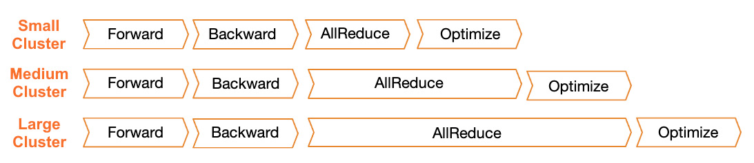
Figure 6.6 – Allreduce times with a cluster increase

To increase training efficiencies, specifically, in a large cluster, SDDP introduces several novel optimizations:

• SDDP utilizes GPU and CPU devices during training, so GPU devices perform forward and backward passes, and CPU devices perform gradient averaging and communication with other training processes during the allreduce stage. This approach allows you to run compute operations and allreduce in parallel and, hence, maximize utilizations.
• SDDP supports FusionBuffers to balance data sent over the network during allreduce (such as Horovod’s Tensor Fusion feature).

As a result, AWS claims that SDDP provides near linear scaling of training throughput with an increase in the training cluster size. AWS published the following benchmarks to demonstrate the optimization gains of SDDP compared to native PyTorch DDP: for 8 node clusters of p3dn.24xl, SSDP outperforms PyTorch DDP by 41% when training the BERT model and by 13% when training the MaskRCNN model. Please refer to this article for more details: https://docs.aws.amazon.com/sagemaker/latest/dg/data-parallel-intro.html.

When engineering an SDDP training job, keep the following aspects in mind:

• SDDP relies on the CPU device to perform the allreduce operation. Most framework data loaders use CPU, too. So, make sure that you control your CPU usage to avoid overutilization. In Chapter 7, Operationalizing Deep Learning Training, we will discuss tools that you can use to control your resource utilization such as SageMaker Debugger. Alternatively, you can move data loading operations to GPU. However, in this case, you will have less available GPU memory to load the model and run its forward and backward passes.
• SDDP might not have significant or any benefits when used in small clusters or on a single node, as it was designed to specifically address the bottlenecks of large training clusters.

Let’s review an example of an SDDP-based training job. For this, we will reuse the previous PyTorch DDP and make minimal modifications to switch from PyTorch DDP to the SDDP library.

As a training task, we use the same binary classification CV as in the PyTorch DDP sample. Since SDDP is natively supported by SageMaker, we don’t need to develop any custom launcher utilities. SDDP uses the mpirun utility to spawn training processes in our cluster. You can use the distribution parameter to enable data-parallel execution and provide any mpi options, as follows:

distribution = { 
    "smdistributed": { 
        "dataparallel": {
            "enabled": True, 
            "custom_mpi_options": "-verbose -x NCCL_DEBUG=VERSION"
        }
    }
}

Now, let’s move on to adopting the training script.

Adopting the training script

SDDP’s starting version 1.4.0 is an integrated PyTorch DDP package that we used in the previous example as a specific backend option. This significantly reduces the changes needed to use SDDP. In fact, if you already have a DDP-enabled training script, you will only need to add an import of the torch_sddp package and use the smddp communication backend when initializing the process group, as follows:

import smdistributed.dataparallel.torch.torch_smddp
import torch.distributed as dist
dist.init_process_group(backend='smddp')

Keep in mind that SDDP v1.4 is only available with the latest PyTorch v10 DL containers. For earlier versions, the SDDP API is slightly different. For more details, please refer to the official API documentation at https://sagemaker.readthedocs.io/en/stable/api/training/distributed.html#the-sagemaker-distributed-data-parallel-library.

Running the SDDP SageMaker training job

Starting the SDDP job requires you to provide a special distribution object with the configuration of data parallelism. Another thing to keep in mind is that SDDP is only available for a limited set of multi-GPU instance types: ml.p3.16xlarge, ml.p3dn.24xlarge, and ml.p4d.24xlarge. Take a look at the following:

from sagemaker.pytorch import PyTorch
instance_type = 'ml.p3.16xlarge'
instance_count = 2
distribution = { 
    "smdistributed": { 
        "dataparallel": {
            "enabled": True, 
            "custom_mpi_options": "-verbose -x NCCL_DEBUG=VERSION"
        }
    }
}
sm_dp_estimator = PyTorch(
          entry_point="train_sm_dp.py",
          source_dir='3_sources',
          role=role,
          instance_type=instance_type,
          sagemaker_session=sagemaker_session,
          framework_version='1.10',
          py_version='py38',
          instance_count=2,
          hyperparameters={
              "batch-size":64,
              "epochs":25,
          },
          disable_profiler=True,
          debugger_hook_config=False,
          distribution=distribution,
          base_job_name="SM-DP",
      )

Note that since we are using a small dataset, this training sample won’t be indicative of any performance efficiencies of SDDP compared to the open source data parallel frameworks.

Summarizing data parallelism

So far, we have discussed how to speed up the training of DL models, which can fit into the memory of an individual device. We discussed and developed training scripts using native implementations as part of the DL frameworks, open source, and proprietary cross-framework Allreduce implementations (Horovod and SageMaker SDDP, respectively). However, we didn’t attempt to benchmark the training efficiencies of the given implementation. While each use case is unique, the general recommendation would be to consider SDDP as a first choice when you are dealing with large-scale and lengthy training processes involving large clusters. If you have a medium- or small-scale training job, you still might consider using framework-native data-parallel implementations. In such cases, the SDDP performance benefits can be negligible.

In the next section, we will discuss how to optimally train models that cannot fit into single GPU memory using model parallelism.

Engineering model parallel training jobs

In model parallelism, a single copy of the model is distributed across two or more training devices to avoid the memory limitations of a single GPU device. A simple method of model parallelism is to explicitly assign layers of the model onto different devices. In this case, forward pass computations will be performed on the GPU device storing the first set of layers. Then, the results will be transferred to the GPU device storing the next set of layers, and so on. The handoff between layers will happen in reverse order during the backward pass. This type of model parallelism is known as naïve model parallelism or vertical model parallelism because we split the model vertically between devices. However, this type of model parallelism is inefficient, as each GPU device will wait for a significant amount of time for other devices to complete their computations. A more efficient way to organize model parallelism is called Pipeline Parallelism. This splits a single data batch into a number of micro-batches and tries to minimize the waiting time by overlapping the computing gradients for different micro-batches. See a comparison of naïve model parallelism and pipeline parallelism in Figure 6.7:

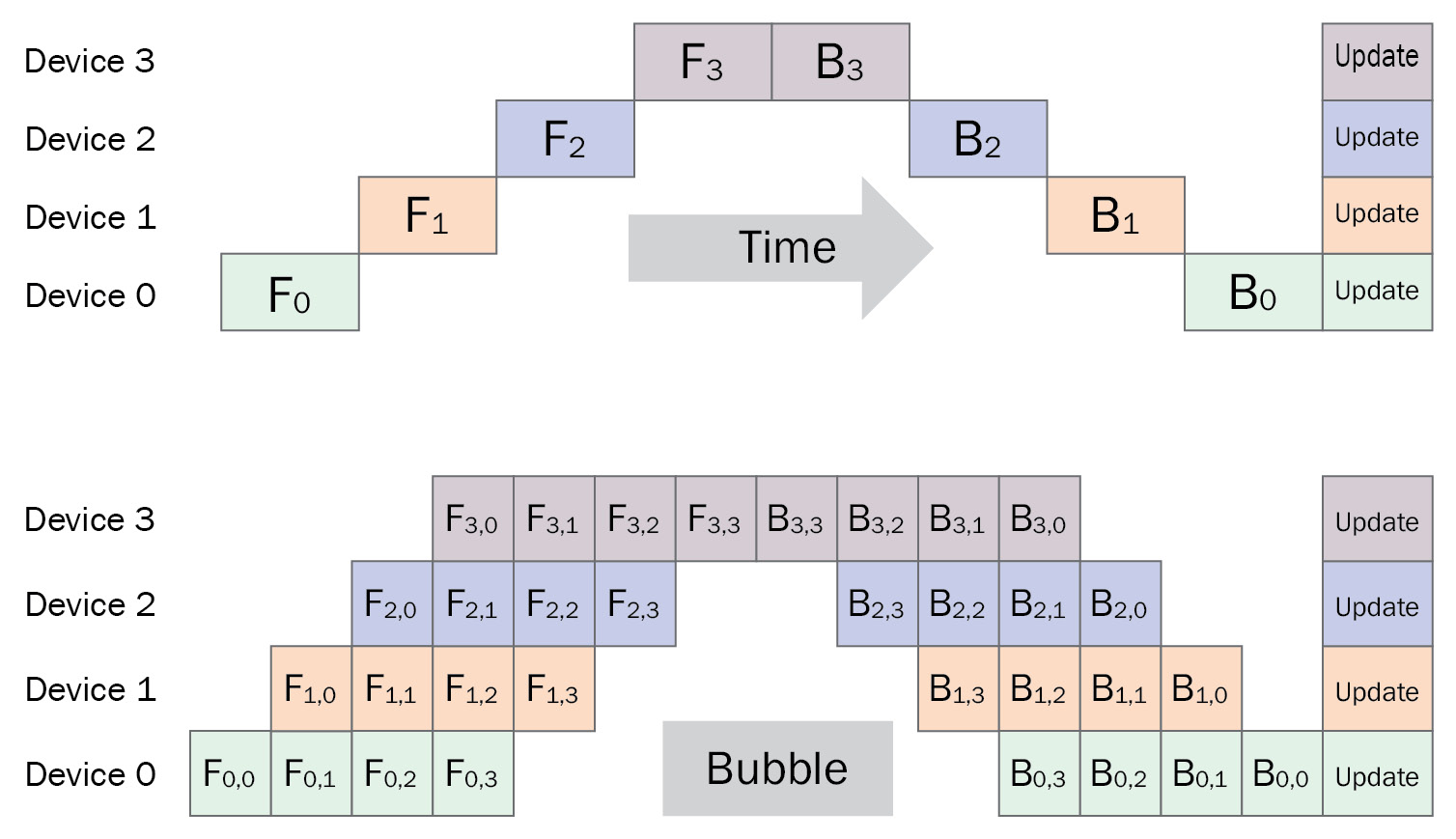
Figure 6 .7 – Naïve model parallelism and pipeline model parallelism

Source of the figure

https://ai.googleblog.com/2019/03/introducing-gpipe-open-source-library.html

Implementing pipeline parallelism has several challenges, as you will likely need to reimplement your training script to assign parts of the model to different devices and reflect the new computation flow in your training loop. Also, you will need to decide how to optimally place your model layers on devices within the same node and across nodes. Additionally, pipeline parallel doesn’t support conditional flows and requires each layer to take a tensor as input and produce a tensor output. You will also need to reimplement pipeline parallelism for each new model architecture. Later in this section, we’ll see how the SMDP library addresses these challenges.

Splitting the model vertically is one way to minimize memory footprint. Another parallelization approach is called Tensor Parallelism. Each tensor (data inputs and layer outputs) is split across multiple devices and processed in parallel. Then, the individual results are aggregated. Tensor parallelism is possible as many compute operations can be represented as matrix operations, which can be split along the X or Y axes. Refer to Figure 6.8 for a visual representation of how tensors can be split. Tensor parallelism is also known as horizontal parallelism:

Figure 6.8 – Row-wise and column-wise tensor parallelism

Source of the figure

https://github.com/huggingface/transformers/blob/main/docs/source/en/perf_train_gpu_many.mdx

Pipeline and tensor model parallelism can be combined. Moreover, data parallelism can be added to achieve even further parallelization and a better training speed. The combination of data parallelism and model parallelism is known as hybrid parallelism. This approach is used to train most of the current large SOTA NLP models such as T5 or GPT3. Refer to Figure 6.9, which illustrates a combination of pipeline parallelism and data parallelism:

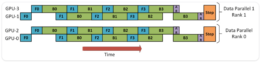
Figure 6.9 – Combining pipeline parallelism and data parallelism

Now that we have refreshed our understanding of key model parallel approaches, let’s review the SDMP library – the SageMaker proprietary implementation of model parallelism.

Engineering training with SDMP

SDMP is a feature-rich library that implements various types of model parallelism and hybrid parallelism and is optimized for the SageMaker infrastructure. It supports the TensorFlow and PyTorch frameworks and allows you to automatically partition models between devices with minimal code changes to your training script. Like SDDP, SDMP uses MPI to coordinate tasks in the training cluster, performing forward and backward computations on GPU devices and communication tasks on CPU devices.

SDMP has a few notable features to simplify the development of model parallel training jobs and optimize hardware utilization at training time:

• SDMP supports arbitrary model architecture and requires minimal code changes to your training script. It doesn’t have any accuracy penalties.
• Automated model splitting partitions your model between devices in the training cluster. You can choose to optimize for speed and memory utilization. Additionally, SDMP supports manual model splitting (however, in practice, this is rarely a good approach).
• Interleaved pipeline is an improvement of simple model pipelining and allows you to minimize the amount of time processing micro-batches by prioritizing backward operations whenever possible:

Figure 6.10 – A comparison of simple and interleaved pipelines

Source of the figure

https://docs.aws.amazon.com/sagemaker/latest/dg/model-parallel-core-features.html

While SDMP officially supports both TensorFlow 2 and PyTorch, certain optimizations are only available for PyTorch. This extended support for PyTorch includes the following:

• Optimizer state sharding allows you to split not only the model but also the optimizer state between training devices in data parallel groups. This further reduces the memory footprint of individual devices during training. Note that optimizer state sharding adds an aggregation step (when the global optimizer state is reconstructed from individual shards), which will result in additional latency.
• Tensor parallelism in addition to pipeline and data parallelism. Tensor parallelism can be specifically useful for large layers that cannot fit into a single GPU device, such as embeddings.
• Activation checkpointing and activation offloading are two other techniques that further minimize the training memory footprint in exchange for some additional compute time to reconstruct the training state.

As using these advanced optimization features comes with a memory-compute trade-off, it’s generally advised that you only use them for large models (that is, billions of parameters).

Now, let’s develop a hybrid parallel job using the SDMP library. We will reuse the previous PyTorch example with CV models.

Note

This example has an educational purpose only. Usually CV models (such as Resnet18) can fit into a single GPU, and in this case, model parallelism is not required. However, smaller models are easy to manage and quick to train for demo purposes.

Configuring model and hybrid parallelism

First, let’s understand how our training will be executed and how we can configure parallelism. For this, we will use the distribution object of the SageMaker training job. It has two key components: model parallel and mpi.

SageMaker relies on the mpi utility to run distributed computations. In the following code snippet, we set it to run 8 training processes. Here, processes_per_host defines how many training processes will be run per host, which includes both processes running model parallelism, data parallelism, or tensor parallelism. In most cases, the number of processes should match the number of available GPUs in the node.

The Modelparallel object defines the configuration of the SDMP library. Then, in the code snippet, we set 2-way model parallelism (the partitions parameter is set to 2). Also, we enable data parallelism by setting the ddp parameter to True. When data parallelism has been enabled, SDMP will automatically infer the data parallel size based on the number of training processes and the model parallelism size. Another important parameter is auto_partition, so SDMP automatically partitions the model between GPU devices.

In the following code block, we configure our training job to run on 2 instances with a total of 16 GPUs in the training cluster. Our distribution object defines 2-way model parallelism. Since the total number of training processes is 16, SDMP will automatically infer 8-way data parallelism. In other words, we split our model between 2 GPU devices, and have a total of 8 copies of the model:

smd_mp_estimator = PyTorch(
# ... other job parameters are reducted for brevity
instance_count=2,
instance_type= 'ml.p3.16xlarge',          
distribution={
                  "modelparallel": {
                      "enabled":True,
                      "parameters": {
                          "microbatches": 8, 
                          "placement_strategy": "cluster", 
                          "pipeline": "interleaved",
                          "optimize": "speed", 
                          "partitions": 2,
                          "auto_partition": True,
                          "ddp": True,
                      }
                  }
              },
            "mpi": {
                    "enabled": True,
                    "processes_per_host": 8,
                    "custom_mpi_options": mpioptions 
              }

Please note that you need to align the configuration of hybrid parallelism with your cluster layout (the number of nodes and GPU devices). SageMaker Python SDK provides upfront validation of the hybrid parallelism configuration; however, this doesn’t guarantee that all your GPU devices will be used during the training process. It’s a good idea to add debug messages to your training scripts to ensure that all GPU devices are properly utilized.

Adopting the training scripts

One of the benefits of SDMP is that it requires minimal changes to your training script. This is achieved by using the Python decorator to define computations that need to be run in a model parallel or hybrid fashion. Additionally, SDMP provides an API like other distributed libraries such as Horovod or PyTorch DDP. In the following code block, we only highlight the key parts. The full source is available at https://github.com/PacktPublishing/Accelerate-Deep-Learning-Workloads-with-Amazon-SageMaker/tree/main/chapter6/4_sources:

1. We start by importing and initializing the SDMP library:

   import smdistributed.modelparallel.torch as smp

   smp.init()

2. Once the library has been initialized, we can use the SDMP API to check that our hybrid parallelism has been correctly configured. For this, you can run the following debug statement as part of your training script:

   logger.debug(

   f"Hello from global rank {smp.rank()}. "

         f"Local rank {smp.local_rank()} and local size {smp.local_size()}. "

         f"List of ranks where current model is stored {smp.get_mp_group()}. "

         f"List of ranks with different replicas of the same model {smp.get_dp_group()}. "

         f"Current MP rank {smp.mp_rank()} and MP size is {smp.mp_size()}. "

           f"Current DP rank {smp.dp_rank()} and DP size is {smp.dp_size()}."

       )

3. The output will be produced in each training process. Let’s review the output from global rank 0. Here, the message prefix in brackets is provided by the MPP utility, marking the unique MPI process, and algo-1 is a reference to the hostname. From the debug message, you can confirm that we have configured 2-way parallelism and 8-way data parallelism. Additionally, we can observe GPU assignments for the data parallel and model parallel groups:

   [1,mpirank:0,algo-1]:INFO:__main__:Hello from global rank 0. Local rank 0 and local size 8. List of ranks where current model is stored [0, 1]. List of ranks with different replicas of the same model [0, 2, 4, 6, 8, 10, 12, 14]. Current MP rank 0 and MP size is 2. Current DP rank 0 and DP size is 8.

4. SDMP manages the assignment of model partitions to the GPU device, and you don’t have to explicitly move the model to a specific device (in a regular PyTorch script, you need to move the model explicitly by calling the model.to(device) method). In each training script, you need to choose a GPU device based on the SMDP local rank:

   torch.cuda.set_device(smp.local_rank())

   device = torch.device("cuda")

5. Next, we need to wrap the PyTorch model and optimizers in SDMP implementations. This is needed to establish communication between the model parallel and data parallel groups.
6. Once wrapped, you will need to use SDMP-wrapped versions of the model and optimizer in your training script. Note that you still need to move your input tensors (for instance, data records and labels) to this device using the PyTorch input_tensor.to(device) method:

   model = smp.DistributedModel(model)

   optimizer = smp.DistributedOptimizer(optimizer)

7. After that, we need to configure our data loaders. SDMP doesn’t have any specific requirements for data loaders, except that you need to ensure batch size consistency. It’s recommended that you use the drop_last=True flag to enforce it. This is because, internally, SDMP breaks down the batch into a set of micro-batches to implement pipelining. Hence, we need to make sure that the batch size is always divisible by the micro-batch size. Note that, in the following code block, we are using the SDMP API to configure a distributed sampler for data parallelism:

       dataloaders_dict = {}

       train_sampler = torch.utils.data.distributed.DistributedSampler(

           image_datasets["train"], num_replicas=sdmp_args.dp_size, rank=sdmp_args.dp_rank)

       dataloaders_dict["train"] = torch.utils.data.DataLoader(

           image_datasets["train"],

           batch_size=args.batch_size,

           shuffle=False,

           num_workers=0,

           pin_memory=True,

           sampler=train_sampler,

           drop_last=True,

       )

       dataloaders_dict["val"] = torch.utils.data.DataLoader(

           image_datasets["val"],

           batch_size=args.batch_size,

           shuffle=False,

           drop_last=True,

       )

8. Once we have our model, optimizer, and data loaders configured, we are ready to write our training and validation loops. To implement model parallelism, SDMP provides a @smp.step decorator. Any function decorated with @smp.set splits executes internal computations in a pipelined manner. In other words, it splits the batch into a set of micro-batches and coordinates the computation between partitions of models across GPU devices. Here, the training and test computations are decorated with @smp.step. Note that the training step contains both forward and backward passes, so SDMP can compute gradients on all partitions. We only have the forward pass in the test step:

   @smp.step

   def train_step(model, data, target, criterion):

       output = model(data)

       loss = criterion(output, target)

       model.backward(loss)  #  instead of PyTorch loss.backward()

       return output, loss

   @smp.step

   def test_step(model, data, target, criterion):

       output = model(data)

       loss = criterion(output, target)

       return output, loss

Note another difference: when calculating loss, we used the model.backward(loss) SDMP method. So, SDMP can correctly compute gradient values across model partitions.

9. We use decorated training and test steps in the outer training loop as follows. The training loop construct is like a typical PyTorch training loop with one difference. Since SDMP implements pipelining over micro-batches, the loss values will be calculated for micro-batches, too (that is, the loss_mb variable). Hence, to calculate the average loss across the full batch, we call the reduce_mean() method. Note that all variables returned by the @smp.step decorated function are instances of the class that provides a convenient API to act across mini-batches (such as the .reduce_mean() or .concat() methods):

   for epoch in range(num_epochs):

           for phase in ["train", "val"]:

               if phase == "train":

                   model.train()  # Set model to training mode

               else:

                   model.eval()  # Set model to evaluate mode

               for inputs, labels in dataloaders[phase]:

                   inputs = inputs.to(device)

                   labels = labels.to(device)

                   optimizer.zero_grad()

                   with torch.set_grad_enabled(phase == "train"):

                       if phase == "train":

                           outputs, loss_mb = train_step(model, inputs, labels, criterion)

                           loss = loss_mb.reduce_mean()

                           optimizer.step()

                       else:

                           outputs, loss_mb = test_step(model, inputs, labels, criterion)

                           loss = loss_mb.reduce_mean()

10. Once training is done, we need to save our distributed model. For this, SMDP provides the smp.save() method, which supports saving both the model and optimizer states in pickle format. You can choose whether you want to persist model partitions or not by using the partial flag. If partial saving is enabled, then the model partitions are saved separately along with their model parallel ranks. In the following code block, we save a single model checkpoint. Note that we are saving the model in a single process based on the rank filter to avoid any conflicts:

        if smp.dp_rank() == 0:

            model_file_path = os.path.join(

                os.environ["SM_MODEL_DIR"], f"finetuned-{args.model_name}-checkpoint.pt"

            )

            model_dict = model.state_dict()  # save the full model

            opt_dict = optimizer.state_dict()  # save the full optimizer state

            smp.save(

                {"model_state_dict": model_dict, "optimizer_state_dict": opt_dict},

                model_file_path,

                partial=False,

            )

11. Once our testing is complete, SageMaker will upload the model and optimizer checkpoints to the S3 location. You can use this model for inference as follows:

    model_state = torch.load('finetuned-resnet-checkpoint.pt')['model_state_dict']

    model_ft = models.resnet18(pretrained=False)

    num_ftrs = model_ft.fc.in_features

    model_ft.fc = nn.Linear(num_ftrs, num_classes)

    model_ft.load_state_dict(model_state)

    outputs = model_ft(inputs)

These are the minimal changes that are required in your training script to make it compatible with the SDMP library to implement model or hybrid parallelism. We encourage you to experiment with various SDMP configuration parameters (please refer to the distribution object from the previous section) to develop good intuition, specifically the following:

• Change the number of model partitions. Our implementation has 2 partitions; you might try to set 1 or 4 partitions and see how this changes the data parallel and model parallel groups.
• Change the number of micro-batches and batch size to see how it impacts training speed. In production scenarios, you will likely need to explore an upper memory limit for batch size and micro-batches to improve training efficiency.
• See how the type of pipeline implementation – interleaved or simple – impacts the training speed.

Additional considerations

We used relatively simple and small models such as Resnet to demonstrate how to implement hybrid parallelism. However, the implementation of more complex models such as GPT-n will require additional considerations. The following sections detail them.

Tensor parallelism

Tensor parallelism is only available in the PyTorch version of the SDMP library. Tensor parallelism makes sense to use for scenarios when a parameter layer consumes a considerable amount of GPU memory (such as embedding tables). When using tensor parallelism, you need to make sure that SDMP supports the modules of your model. SDMP provides distributed implementations of common modules such as nn.Linear, nn.Embedding, and more. If a specific module is not supported, first, you will need to implement a tensor-parallelizable version of it. Please refer to the SDMP API documentation for details: https://sagemaker.readthedocs.io/en/stable/api/training/smp_versions/latest/smd_model_parallel_pytorch_tensor_parallel.html.

Reference implementations

AWS provides a few example scripts to train popular large models such as GPT2, GPT-J, and BERT using the SDMP library. See the official GitHub repository at https://github.com/aws/amazon-sagemaker-examples/tree/main/training/distributed_training/pytorch/model_parallel.

You can also find the reference configuration of SDMP at https://docs.aws.amazon.com/sagemaker/latest/dg/model-parallel-best-practices.html.

So far, we have covered different ways to distribute your training job and looked at sample implementations. In the next section, we will cover some parameters to improve the efficiency of your distributed training job.

Optimizing distributed training jobs

In many cases, optimizing your large-scale distributed training jobs requires a lot of trial and error and is very specific to the runtime environment, hardware stack, model architecture, and other parameters. But there are several key knobs that might help to optimize your training speed and overall efficiency.

Cluster layout and computation affinity

When running distributed training jobs, especially model parallel or hybrid parallel, it’s always a good idea to understand how different types of computation are aligned with your cluster layout.

Let’s consider a situation when we need to run model parallel training in the cluster of two nodes with two GPU devices each. The total training processes count is 4 with global ranks ranging from 0 to 3 and local ranks being 0 and 1. We assume that the model copy and gradients can fit into two devices. In this case, we need to ensure that each model will be stored within each node: one model copy will be placed on ranks 0 and 1 (local ranks 0 and 1), and another on ranks 2 and 3 (local ranks 0 and 1). This will ensure that communication between layers of the model will happen over faster inter-GPU connections and won’t, typically, traverse slower intra-node networks.

To address this situation, SDMP provides a special parameter called placement_strategy, which allows you to control the training process’s affinity to your hardware.

Communication backend

In this chapter, we covered some of the most popular communication backends, such as NCCL, Gloo, and MPI. The following list is a rule of thumb when choosing which backend to use given your specific case:

• Message passing interface (MPI) is a communication standard in distributed computations that comes with a number of backend implementations, such as Open-MPI, MVAPICH2, and more. MPI backends also support inter-GPU operations on CUDA tensors. However, MPI is rarely an optimal choice for your training job if you have other options.
• Gloo backends come with wide support for point-to-point and collective computations between CPU devices as well as collective computations between GPU devices. Gloo can be a good choice for initial debugging on CPU devices. However, you should usually prefer NCCL when using GPU devices for training.
• NCCL backends are provided by NVIDIA and are optimal for training jobs on NVIDIA GPUs.
• Custom backends can be provided as part of the DL framework. For instance, TensorFlow 2 provides a custom RING backend.

Note

When working with a newer SOTA model, make sure that the communication backend of your choice supports the collective and point-to-point operations required by your model architecture.

Training hyperparameters

There are many training hyperparameters that can impact your training efficiencies. While we don’t intend to cover all of them, we have listed some hyperparameters that you can tweak in your optimization efforts:

• Use AMP to reduce memory requirements and speed up training with minimal impact on accuracy and training convergence. AMP is a popular technique that is used to combine single (FP32) and half-precision (FP16) tensors during the forward, backward, and update steps. Note that you will likely need to have a large batch size in order to have meaningful improvements with AMP.
• Use hardware-optimized data types (such as TF32, BF32, and BF16) to speed up training. These data types are optimized for specific DL computations and provide speed up compared to the common FP32 and FP16 types. Note that to use these types, you need to ensure that your framework, model architecture, and hardware support it.
• Optimize your global batch size to speed up training. As you scale out your training cluster, make sure that you are updating your global batch size accordingly. Typically, the upper limit of local batch size is defined by available GPU memory (you will likely see a CUDA OOM error if the local batch size cannot fit into memory). Keep in mind that increasing the batch size beyond a certain threshold might not increase the global training throughput either. You can find some additional materials and benchmarks in the NVIDIA guide at https://docs.nvidia.com/deeplearning/performance/dl-performance-fully-connected/index.html#batch-size. Another thing to keep in mind is that you might need to proportionally increase the learning rate with an increase in the batch size.
• Use fused optimizers (such as the FusedAdam optimizer) to speed up weight updates using the operation fusion – combining multiple operations into one. Make sure that you confirm that your DL framework and hardware support fused optimizers.

These are several common parameters that might improve the efficiency of your training jobs. Note that, in many real-life use cases, you might have model- or task-specific tuning parameters.

Summary

In this chapter, we focused on how to engineer large-scale data parallel, model parallel, and hybrid distributed training jobs. We discussed which type of parallelism to choose based on your specific use case and model architecture. Then, we reviewed several popular approaches of how to organize distributed training – such as the Parameter Server and Allreduce algorithms – along with various performance considerations to tune distributed training jobs. You will now be able to select the correct type of distributed training, technical stack, and approach to debug and tune training job performance. Then, we reviewed several examples of distributed training jobs in Amazon SageMaker using the popular open source and proprietary libraries SDDP and SMDP.

Running large-scale training jobs requires not only initial engineering efforts but also the well-established operational management of your training jobs. In many cases, the training job can run for days and weeks, or you will need to periodically retrain your models on new data. As each long-running DL training job requires considerable compute resources and associated time and cost resources, we want to make sure that our training is efficient. For instance, we need to control in real time whether our model is converging during training. Otherwise, we might want to stop earlier and avoid wasting compute resources and time. In the next chapter, we will focus on setting up an operational stack for your DL training jobs.