9

Implementing Model Servers

In Chapter 8, Considering Hardware for Inference, we discussed hardware options and optimizations for serving DL models that are available to you as part of the Amazon SageMaker platform. In this chapter, we will focus on another important aspect of engineering inference workloads – choosing and configuring model servers.

Model servers, similar to application servers for regular applications, provide a runtime context to serve your DL models. You, as a developer, deploy trained models to the model server, which exposes the deployed models as REST or gRPC endpoints. The end users of your DL models then send inference requests to established endpoints and receive a response with predictions. The model server can serve multiple end users simultaneously. It also provides configurable mechanisms to optimize inference latency and throughput to meet specific SLAs.

In Chapter 1, Introducing Deep Learning with Amazon SageMaker, we discussed that Amazon SageMaker Managed Hosting has several mechanisms to deploy models: real-time inference endpoints, batch transform jobs, and asynchronous inference. In all these cases, you will need to select a model server to manage inference runtime and model deployment. However, model server configuration for these use cases will likely be different, since they have different inference traffic profiles and latency/throughput requirements.

Amazon SageMaker provides several model server solutions as part of its DL Inference Containers. In this chapter, we will focus on three popular model servers designed to productionalize DL inference workloads: TensorFlow Serving (TFS), PyTorch TorchServe (PTS), and NVIDIA Triton.

In this chapter, we will cover the following topics:

• Using TFS
• Using PTS
• Using NVIDIA Triton

After reading this chapter, you will know how to deploy your TensorFlow and PyTorch models and configure your model servers for your inference requirements. We will also discuss the functional limitations of using model servers as part of SageMaker Managed Hosting.

Technical requirements

In this chapter, we will provide code samples so that you can develop practical skills. The full code examples are available here: https://github.com/PacktPublishing/Accelerate-Deep-Learning-Workloads-with-Amazon-SageMaker/blob/main/chapter9/.

To follow along with this code, you will need the following:

• An AWS account and IAM user with permission to manage Amazon SageMaker resources.
• Have a SageMaker Notebook, SageMaker Studio Notebook, or local SageMaker-compatible environment established.
• Access to GPU training instances in your AWS account. Each example in this chapter will provide the recommended instance types for you to use. You may need to increase your compute quota for SageMaker Training Job to have GPU instances enabled. In this case, please follow the instructions at https://docs.aws.amazon.com/sagemaker/latest/dg/regions-quotas.html.
• You must install the required Python libraries by running pip install -r requirements.txt. The file that contains the required libraries can be found in the chapter9 directory.
• In this chapter, we will provide examples of compiling models for inference, which requires access to specific accelerator types. Please review the instance recommendations as part of the model server examples.

Using TFS

TFS is a native model server for TensorFlow 1, TensorFlow 2, and Keras models. It is designed to provide a flexible and high-performance runtime environment with an extensive management API and operational features (such as logging and metrics). AWS provides TFS as part of TensorFlow inference containers (https://github.com/aws/deep-learning-containers/tree/master/tensorflow/inference/docker).

Reviewing TFS concepts

TFS has a concept known as servable that encapsulates all model and code assets required for inference. To prepare servable for TFS serving, you need to package the trained model into SavedModel format. A SavedModel contains a complete TensorFlow program, including trained parameters and computation. It does not require the original model building code to run, which makes it useful for sharing or deploying across the TFS ecosystem (for example, using TFLite, TensorFlow.js, or TFS). You can package more than one model as well as specific model lookups or embeddings in a single servable.

TFS loads and exposes your servable via REST or gRPC endpoints. The Server API defines a list of endpoints to perform classification and regression inference. Additionally, each servable has an associated signature that defines the input and output tensors for your model, as well as the model type (regression or classification). Many common models have standard signatures that depend on the type of task (for example, image classification, object detection, text classification, and so on). TFS allows you to have custom signatures as well.

Integrating TFS with SageMaker

Amazon SageMaker provides a managed hosting environment where you can manage your inference endpoints with uniform management and invocation APIs, regardless of the underlying model server. This approach sets certain limitations on native model server functionality. In this section, we will review how SageMaker integrates with TFS and the limitations you should be aware of.

When deploying TFS on SageMaker, you will not have access to TFS’s native management API to manage your servable life cycle (loading and unloading models, promoting the model version, and more). Also, you will not have direct access to the TFS Serving API. Instead, you will need to call your SageMaker endpoint using the standard SageMaker invocation interface. Then, the SageMaker HTTP server (a part of the DL TFS container) translates your requests into TFS format and passes them to the TFS Serving APIs. Note that you can provide custom pre-processing, prediction, and post-processing logic in your inference script. SageMaker supports both the REST and gRPC serving APIs. The following diagram shows this TFS integration:

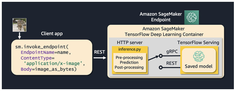
Figure 9.1 – TFS integration with SageMaker Managed Hosting

There are several things to keep in mind when working with TFS on SageMaker:

• As mentioned previously, SageMaker doesn’t allow you to access the TFS Management API. However, it does allow to you provide the configuration of TFS via environmental variables.
• SageMaker supports hosting multiple models with TFS. For this, you need to prepare separate servables for each model and then create a multi-model archive.
• You can use REST headers and a request body to specify which models TFS should use to serve specific requests. For instance, the following request tells TFS to use model2 to serve this request:

  aws sagemaker-runtime invoke-endpoint

      --endpoint-name my-endpoint

      --content-type 'application/json'

      --body '{"instances": [1.0, 2.0, 5.0]}'

      --custom-attributes 'tfs-model-name=other_model

SageMaker supports default TFS input and output formats for your inference requests. Additionally, SageMaker also supports application/JSON, text/CSV, and application/JSON Lines.

Note that once you deploy the endpoint with the TFS model server, you won’t be able to directly change the TFS configuration or served models. For this, you will need to use the SageMaker Management API to create a new endpoint or endpoint variant with the desired configuration. We will discuss managing SageMaker inference resources in production in Chapter 10, Operationalizing Inference Workloads.

Optimizing TFS

TFS provides a set of mechanisms to optimize your model serving based on your requirements, the runtime environment, and available hardware resources. It implies that TFS tuning is use-case-specific and typically requires testing and benchmarking to achieve desired performance. In this section, we will review several mechanisms that you can use to tune TFS performance.

Using TFS batching

TFS supports automatic batching, where you can put several inference requests in a single batch. This can improve your server throughput, especially when using GPU instances (remember, GPUs are very good for parallel computations). How you configure batching will be different depending on the type of hardware device. TFS supports different batching schedules for different servables.

To configure TFS batching on SageMaker, you can use the following environment variables:

• SAGEMAKER_TFS_ENABLE_BATCHING to enable the TFS batching feature. This defaults to false, which means that batching is not enabled.
• SAGEMAKER_TFS_MAX_BATCH_SIZE defines the maximum size of the batch. This defaults to 8.
• SAGEMAKER_TFS_BATCH_TIMEOUT_MICROS defines how long to wait to accumulate a full batch in microseconds. This defaults to 1000.
• SAGEMAKER_TFS_NUM_BATCH_THREADS sets how many batches to process simultaneously. This defaults to the number of instance CPUs.
• SAGEMAKER_TFS_MAX_ENQUEUED_BATCHES defines how many batches can be enqueued at the same time.

You can review the detailed documentation on the TFS batching feature here: https://github.com/tensorflow/serving/blob/master/tensorflow_serving/batching/README.md.

Using the gRPC serving API

As discussed earlier, TFS supports two types of APIs: REST and gRPC. While both APIs have the same functionality, the gRPC API typically has better performance due to the use of HTTP/2 network protocol and more efficient payload representations via the ProtoBuf format.

While the SageMaker Invocation API only supports the REST API, you can still use gRPC for inter-container communication between SageMaker’s HTTP frontend server and TFS (refer to Figure 9.1 for an illustration of this). Note that in this case, you will need to provide some code to translate the SageMaker payload into gRPC format and send it to TFS. However, even in this case, AWS reports a decrease in the overall latency by at least 75% for image classification tasks. Refer to this article for details: https://aws.amazon.com/blogs/machine-learning/reduce-compuer-vision-inference-latency-using-grpc-with-tensorflow-serving-on-amazon-sagemaker/. The performance benefits will vary based on the model and payload size.

Configuring resource utilization with TFS

TFS provides the following parameters for configuring hardware resources allocation:

• SAGEMAKER_TFS_INSTANCE_COUNT defines how many instances of the TFS serving process will be spawned. Changing this parameter may increase your CPU and GPU utilization and ultimately improve your latency/throughput characteristics.
• SAGEMAKER_TFS_FRACTIONAL_GPU_MEM_MARGIN defines the fraction of GPU memory available to initialize the CUDA/cuDNN library. The remaining memory will be distributed equally between TFS processes.
• SAGEMAKER_TFS_INTER_OP_PARALLELISM determines how many threads are used when running independent non-blocking compute operations in your model graphs.
• SAGEMAKER_TFS_INTRA_OP_PARALLELISM determines how many threads are used when running operations that can be parallelized interally.

Now, let’s review how we can use TFS on SageMaker using a practical example.

Implementing TFS serving

In this example, we will take one of the pre-trained models from TensorFlow Hub, convert it into SavedModel format, and then package it with the custom inference for deployment on SageMaker. We will review how we can use both the REST and gRPC APIs and how to define the TFS configuration when it’s deployed on SageMaker Managed Hosting. For this task, we will use the popular EfficientNetV2 model architecture to classify images.

The full code is available here: https://github.com/PacktPublishing/Accelerate-Deep-Learning-Workloads-with-Amazon-SageMaker/blob/main/chapter9/1_TensorFlow_Serving.ipynb.

Preparing the training model

We will start by loading the model artifacts from TensorFlow Hub. You can read about the EfficientNetV2 model on its model page here: https://tfhub.dev/google/imagenet/efficientnet_v2_imagenet1k_s/classification/2. To download the model, we can use the TensorFlow Hub API, as shown in the following code block:

import tensorflow as tf
import tensorflow_hub as hub
model_handle = "https://tfhub.dev/google/imagenet/efficientnet_v2_imagenet1k_s/classification/2"
classifier = hub.load(model_handle)

This model expects a dense 4D tensor of the float32 dtype with a shape of [batch, height, weight, color], where height and weight have a fixed length of 384, and color has a length of 3. batch can be variable.

To test the model locally, you need to convert the image (or a batch of images) into the expected 4D tensor, run it through the model, and apply the softmax function to get the label probabilities, as shown here:

probabilities = tf.nn.softmax(classifier(image)).numpy()

Now that we have performed smoke testing on the model, we need to package it in SageMaker/TFS-compatible formats.

Packaging the model artifacts

As discussed earlier, TFS expects your model to be converted into SavedModel format. Additionally, SageMaker expects the model artifact to be packaged into a tar.gz archive with the following structure:

    model1
        |--[model_version_number]
            |--variables
            |--saved_model.pb
    model2
        |--[model_version_number]
            |--assets
            |--variables
            |--saved_model.pb
    code
        |--inference.py
        |--requirements.txt

The following code creates the appropriate directory structure and exports the trained model in SavedModel format:

model_name = "efficientnetv2-s"
model_dir = f"./{model_name}/1"
code_dir = f"./{model_name}/code"
os.makedirs(model_dir, exist_ok=False)
os.makedirs(code_dir, exist_ok=False)
tf.saved_model.save(classifier, model_dir)

Note that in our example, we will only use a single version of a single model. Next, we need to prepare an inference script for preprocessing, running predictions, and postprocessing between the SageMaker HTTP frontend and the TFS server.

Developing the inference code

SageMaker expects your processing code to be named inference.py and placed in the /code directory in the model archive. Our inference code needs to implement either the input_handler() and output_handler() functions or a single handler() function. In our case, we have chosen to implement a single handler() method to process incoming requests and send it to the appropriate TFS API:

def handler(data, context):
    if context.request_content_type == "application/json":
        instance = json.loads(data.read().decode("utf-8"))
    else:
        raise ValueError(
            415,
            'Unsupported content type "{}"'.format(
                context.request_content_type or "Unknown"
            ),
        )
    if USE_GRPC:
        prediction = _predict_using_grpc(context, instance)
    else:
        inst_json = json.dumps({"instances": instance})
        response = requests.post(context.rest_uri, data=inst_json)
        if response.status_code != 200:
            raise Exception(response.content.decode("utf-8"))
        prediction = response.content
    response_content_type = context.accept_header
    return prediction, response_content_type

As you can see, depending on whether we want to use the gRCP API or the REST API, the processing and prediction code will be slightly different. Note that the context namedtuple object provides necessary details about the TFS configuration, such as the endpoint path and ports, model name and version, and more.

If we choose to use the TFS REST API, we need to convert the incoming request into the expected TFS format, serialize it into JSON, and then generate a POST request.

To use the gRPC API, we will need to convert the incoming REST payload into a protobuf object. For this, we will use the following helper function:

from tensorflow_serving.apis import predict_pb2
from tensorflow_serving.apis import prediction_service_pb2_grpc
def _predict_using_grpc(context, instance):
    grpc_request = predict_pb2.PredictRequest()
    grpc_request.model_spec.name = "model"
    grpc_request.model_spec.signature_name = "serving_default"
    options = [
        ("grpc.max_send_message_length", MAX_GRPC_MESSAGE_LENGTH),
        ("grpc.max_receive_message_length", MAX_GRPC_MESSAGE_LENGTH),
    ]
    channel = grpc.insecure_channel(f"0.0.0.0:{context.grpc_port}", options=options)
    stub = prediction_service_pb2_grpc.PredictionServiceStub(channel)
grpc_request.inputs["input_1"].CopyFrom(tf.make_tensor_proto(instance))
    result = stub.Predict(grpc_request, 10)
    output_shape = [dim.size for dim in result.outputs["output_1"].tensor_shape.dim]
    np_result = np.array(result.outputs["output_1"].float_val).reshape(output_shape)
    return json.dumps({"predictions": np_result.tolist()})

Here, we use the prediction_service_pb2() and predict_pb2() TFS methods to communicate with the gRPC API. Here, the stub object converts parameters during the RPC. The grpc_request object defines what TFS API to invoke and call the parameters.

To choose what TFS API to call, we implemented a simple mechanism that allows you to provide the USE_GRPC environment variable via a SageMaker Model object:

USE_GRPC = True if os.getenv("USE_GRPC").lower() == "true" else False 

Once we have our inference.py code ready, we can add it to the model package and create a tar.gz model archive. This can be done by running the following Bash code from a Jupyter notebook:

! cp 1_src/inference.py $code_dir
! cp 1_src/requirements.txt $code_dir
! tar -C "$PWD" -czf model.tar.gz  efficientnetv2-s/

Now, our model has been packaged according to TFS and SageMaker requirements and we are ready to deploy it.

Deploying the TFS model

To deploy the TFS model, follow these steps:

1. We will start by uploading our model archive to Amazon S3 so that SageMaker can download it to the serving container at deployment time. We can use a SageMaker Session() object to do this:

   import sagemaker

   from sagemaker import get_execution_role

   sagemaker_session = sagemaker.Session()

   role = get_execution_role()

   bucket = sagemaker_session.default_bucket()

   prefix = 'tf-serving'

   s3_path = 's3://{}/{}'.format(bucket, prefix)

   model_data = sagemaker_session.upload_data('model.tar.gz',

                                              bucket,

                                              os.path.join(prefix, 'model'))

2. Then, we can use the SageMaker SDK TensorFlowModel object to configure the TFS environment. Note that we are providing the TFS configuration via the env dictionary:

   from sagemaker.tensorflow import TensorFlowModel

   env = {

          "SAGEMAKER_TFS_ENABLE_BATCHING":"true",

          "SAGEMAKER_TFS_MAX_BATCH_SIZE":"4",

          "SAGEMAKER_TFS_BATCH_TIMEOUT_MICROS":"100000",

          "SAGEMAKER_TFS_NUM_BATCH_THREADS":"6",

          "SAGEMAKER_TFS_MAX_ENQUEUED_BATCHES":"6",

          "USE_GRPC":"true" # to switch between TFS REST and gRCP API

          }

   tensorflow_serving_model = TensorFlowModel(model_data=model_data,

                                    name="efficientnetv2-1",

                                    role=role,

                                    framework_version='2.8',

                                    env=env,

   sagemaker_session=sagemaker_session)

Once the model has been configured, we are ready to deploy the endpoint. Here, we will use one of the GPU instances, but you can experiment with CPU instances as well.

Before we can run predictions, we need to convert the image (or several images) into a 4D TFS tensor and then convert it into a NumPy ndarray that the .predict() method knows how to serialize into the application/JSON content type. A sample method to process images into TFS format has been provided in the sample notebook.

In the following code, we are running predictions and then mapping the resulting softmax scores to labels:

response_remote = predictor.predict(image.numpy())
probabilities = np.array(response_remote['predictions'])
top_5 = tf.argsort(probabilities, axis=-1, direction="DESCENDING")[0][:5].numpy()
np_classes = np.array(classes)
# Some models include an additional 'background' class in the predictions, so
# we must account for this when reading the class labels.
includes_background_class = probabilities.shape[1] == 1001
for i, item in enumerate(top_5):
  class_index = item if includes_background_class else item + 1
  line = f'({i+1}) {class_index:4} - {classes[class_index]}: {probabilities[0][top_5][i]}'
  print(line)

After running this code, you should have an output that contains labels and their normalized probabilities.

In this section, we reviewed how to use the TFS model server on Amazon SageMaker. TFS is a highly configurable production-grade model server that should be considered a great candidate when it comes to hosting TensorFlow models. We also discussed some implementation specifics of Sagemaker/TFS integration that should be accounted for when engineering your model server. Once you have your TensorFlow model(s) running on SageMaker, it’s recommended to perform benchmarking and tune the TFS configuration based on your specific use case requirements.

In the next section, we will review the native model server for PyTorch models – TorchServe.

Using PTS

PTS is a native model server for PyTorch models. PTS was developed in collaboration between Meta and AWS to provide a production-ready model server for the PyTorch ecosystem. It allows you to serve and manage multiple models and serve requests via REST or gRPC endpoints. PTS supports serving TorchScripted models for better inference performance. It also comes with utilities to collect logs and metrics and optimization tweaks. SageMaker supports PTS as part of PyTorch inference containers (https://github.com/aws/deep-learning-containers/tree/master/pytorch/inference/docker).

Integration with SageMaker

PTS is a default model server for PyTorch models on Amazon SageMaker. Similar to TFS, SageMaker doesn’t expose native PTS APIs to end users for model management and inference. The following diagram shows how to integrate SageMaker and PTS:

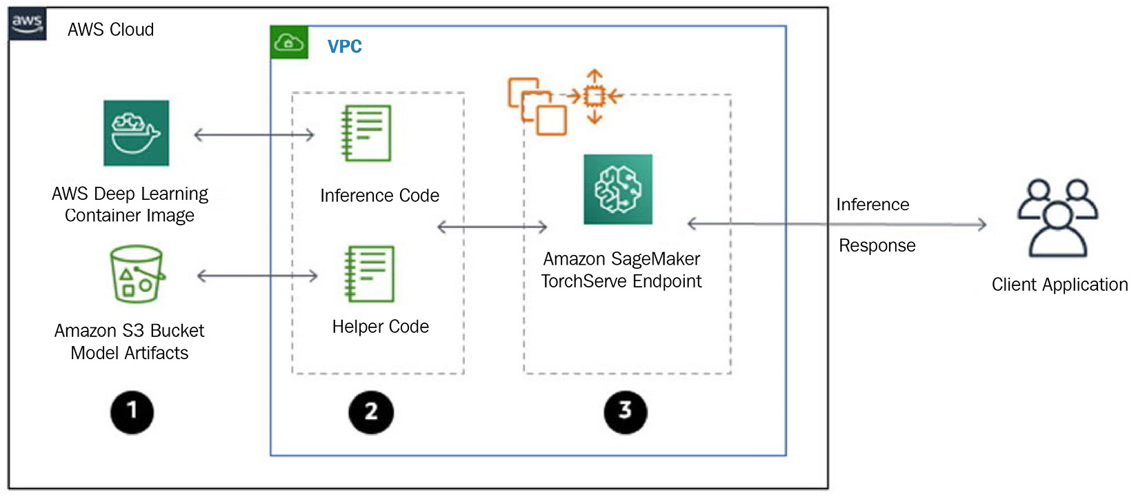
Figure 9.2 – PTS architecture on SageMaker

Let’s highlight these integration details:

• SageMaker supports a limited number of PTS configs out of the box. If you need to have more flexibility with your PTS configuration, you may need to extend the SageMaker PyTorch Inference container. Alternatively, you can package the PTS configs as part of your model package and provide the path to it via the TS_CONFIG_FILE environment variable. However, with the latter approach, you won’t be able to manipulate all the settings (for example, the JVM config).
• PTS requires you to package model artifacts and handler code into a MAR archive. SageMaker has slightly different requirements regarding the model archive, which we will discuss in the following code example.
• SageMaker supports hosting multiple models at the same time. For this, you need to set the ENABLE_MULTI_MODEL environment variable to true and package your models into a single archive.

SageMaker provides a mechanism to configure PTS via endpoint environmental variables. Let’s review the available config parameters.

Optimizing PTS on SageMaker

PTS supports two primary mechanisms for performance optimization: server-side batching and spawning multiple model threads. These settings can be configured via the following environmental variables:

• SAGEMAKER_TS_BATCH_SIZE to set the maximum size of server-side batches.
• SAGEMAKER_TS_MAX_BATCH_DELAY to set the maximum delay that the server will wait to complete the batch in microseconds.
• SAGEMAKER_TS_RESPONSE_TIMEOUT sets the time delay for a timeout in seconds if an inference response is not available.
• SAGEMAKER_TS_MIN_WORKERS and SAGEMAKER_TS_MAX_WORKERS configure the minimum and the maximum number of model worker threads on CPU or GPU devices, respectively. You can read some of the considerations on setting up these in the PyTorch documentation at https://github.com/pytorch/serve/blob/master/docs/performance_guide.md.

Additionally, PTS supports inference profiling using the PyTorch TensorBoard plugin, which we discussed in Chapter 7, Operationalizing Deep Learning Training. This plugin allows you to profile your PyTorch inference code and identify potential bottlenecks.

Serving models with PTS

Let’s review how to deploy PyTorch models using PTS on SageMaker. We will use the Distilbert model that has been trained on the Q&A NLP task from HuggingFace Models. The sample code is available here: https://github.com/PacktPublishing/Accelerate-Deep-Learning-Workloads-with-Amazon-SageMaker/blob/main/chapter9/2_PyTorch_Torchserve.ipynb.

Packaging the model for PTS on SageMaker

When using the PTS model server on SageMaker, you may choose to use one of two options:

• Deploy your model using the PyTorchModel class from the Python SageMaker SDK. In this case, your model archive needs to provide only the necessary model artifacts (for example, model weights, lookups, tokenizers, and so on). As part of the PyTorchModel object configuration, you will provide your inference code and other dependencies, and SageMaker will automatically package it for PTS.
• You can also package your model along with the inference code in a single archive. While this approach requires some additional work, it allows you to create a model package and deploy models without using the SageMaker SDK. SageMaker expects the following directory structure in this case:

  model.tar.gz/

  |- model_weights.pth

  |- other_model_artifacts

  |- code/

    |- inference.py

    |- requirements.txt  # optional

In this example, we will use the first option:

1. The following Bash script will download the required HuggingFace model artifacts and package them into a single tar.gz archive:

   mkdir distilbert-base-uncased-distilled-squad

   wget https://huggingface.co/distilbert-base-uncased-distilled-squad/resolve/main/pytorch_model.bin -P distilbert-base-uncased-distilled-squad

   wget https://huggingface.co/distilbert-base-uncased-distilled-squad/resolve/main/tokenizer.json -P distilbert-base-uncased-distilled-squad

   wget https://huggingface.co/distilbert-base-uncased-distilled-squad/resolve/main/tokenizer_config.json -P distilbert-base-uncased-distilled-squad

   wget https://huggingface.co/distilbert-base-uncased-distilled-squad/resolve/main/vocab.txt -P distilbert-base-uncased-distilled-squada

   wget https://huggingface.co/distilbert-base-uncased-distilled-squad/resolve/main/config.json -P distilbert-base-uncased-distilled-squad

   tar -C "$PWD" -czf distilbert-base-uncased-distilled-squad.tar.gz  distilbert-base-uncased-distilled-squad/

2. Then, we need to upload the model archive to Amazon S3 using the following code:

   import sagemaker

   from sagemaker import get_execution_role

   sagemaker_session = sagemaker.Session()

   role = get_execution_role()

   bucket = sagemaker_session.default_bucket()

   prefix = 'torchserve'

   s3_path = 's3://{}/{}'.format(bucket, prefix)

   model_data = sagemaker_session.upload_data('distilbert-base-uncased-distilled-squad.tar.gz',bucket,os.path.join(prefix, 'model-artifacts'))

Next, we need to prepare some code to load models from the uploaded model artifacts and perform inference and data processing. This code is called the inference handler in PTS terminology.

Preparing the inference handler

SageMaker requires you to provide some code to load the model and run predictions so that you can preprocess incoming inference requests and post-process the response. To perform these operations, you need to implement the model_fn(), predict_fn(), input_fn(), and output_fn() methods. You can find implementations of the inference handler using the HuggingFace Pipeline API here: https://github.com/PacktPublishing/Accelerate-Deep-Learning-Workloads-with-Amazon-SageMaker/blob/main/chapter9/2_src/pipeline_predictor.py.

Deploying the model to a SageMaker endpoint

Deploying the model on PTS using the SageMaker SDK is straightforward. To configure PTS, we can use the "env" dictionary to set the appropriate environment variables in the serving container. Note that here, we explicitly reference the inference code via the "entry_point" parameter. Follow these steps:

1. As a prerequisite, you can add any other dependencies (for example, custom libraries or requirements.txt) to the "source_dir" location. The SageMaker SDK will automatically merge these assets with the model data into the MAR archive required by PTS:

   from sagemaker.pytorch import PyTorchModel

   env = {

       "SAGEMAKER_TS_BATCH_SIZE": "2",

       "SAGEMAKER_TS_MAX_BATCH_DELAY": "1000",

       "SAGEMAKER_TS_RESPONSE_TIMEOUT" : "120",

       "SAGEMAKER_TS_MIN_WORKERS" : "1",

       "SAGEMAKER_TS_MAX_WORKERS" : "2"

       }

   model = PyTorchModel(model_data=model_data,

                      role=role,

                      entry_point='pipeline_predictor.py',

                      source_dir='2_src',

                      framework_version='1.9.0',

                      py_version='py38',

                      env=env,

                      sagemaker_session=sagemaker_session)

2. Now, we can define the endpoint configuration and supported serializers and deserializers for the request/response pair:

   from sagemaker.serializers import JSONSerializer

   from sagemaker.deserializers import JSONDeserializer

   remote_predictor = model.deploy(initial_instance_count=1, instance_type="ml.g4dn.4xlarge", serializer=JSONSerializer(), deserializer=JSONDeserializer())

3. Now, we can run prediction by calling the .predict() method:

   remote_predictor.predict(data)

4. We can also confirm that our PTS configurations have been applied properly. For this, you can open your SageMaker endpoint log stream and search for a log line, as shown here:

   Model config:

   { "model": { "1.0": { "defaultVersion": true, "marName": "model.mar", "minWorkers": 1, "maxWorkers": 2, "batchSize": 3, "maxBatchDelay": 100000, "responseTimeout": 120 } } }

In this section, we discussed how PTS can be used to serve PyTorch models. In real production systems, you will probably prefer to convert your model into TorchScript format and further experiment with batching and worker scaling options to optimize your specific use case requirements.

In the next section, we will review a feature-rich framework-agnostic model server called NVIDIA Triton.

Using NVIDIA Triton

NVIDIA Triton is an open source model server developed by NVIDIA. It supports multiple DL frameworks (such as TensorFlow, PyTorch, ONNX, Python, and OpenVINO), as well various hardware platforms and runtime environments (NVIDIA GPUs, x86 and ARM CPUs, and AWS Inferentia). Triton can be used for inference in cloud and data center environments and edge or mobile devices. Triton is optimized for performance and scalability on various CPU and GPU platforms. NVIDIA provides a specialized utility for performance analysis and model analysis to improve Triton’s performance.

Integration with SageMaker

You can use Triton model servers by utilizing a pre-built SageMaker DL container with it. Note that SageMaker Triton containers are not open source. You can find the latest list of Triton containers here: https://github.com/aws/deep-learning-containers/blob/master/available_images.md#nvidia-triton-inference-containers-sm-support-only.

SageMaker doesn’t require you to provide inference custom code when deploying models on Triton. However, you will need to provide a Triton config.pbtxt file for each model you intend to serve. This config specifies the API contract for the inference request/response pair and other parameters on how the model needs to be served. You can review the possible configuration parameters by reading the official Triton documentation: https://github.com/triton-inference-server/server/blob/main/docs/user_guide/model_configuration.md.

Also, note that, unlike TFS and PTS, at the time of writing, SageMaker doesn’t support hosting multiple independent models on Triton. However, you can still have multiple versions of the same model or organize several models into a pipeline.

Optimizing Triton inference

Triton provides several utilities to improve your performance:

• Model Analyzer allows you to understand the GPU memory utilization of your models so that you can understand how to run multiple models on a single GPU
• Performance Analyzer allows you to analyze your Triton inference and throughput

You won’t be able to run Performance Analyzer directly against SageMaker Triton Endpoint since the SageMaker inference API doesn’t match the Triton inference API. To bypass this limitation, you can run the Triton container locally on an instance of SageMaker Notebook with the target hardware accelerator and run an analysis against it.

Triton provides the following optimization features:

• Dynamic batching: This puts multiple inference requests into a batch to increase Triton throughput. This feature is similar to the batching we discussed for TFS and PTS model servers.
• Model instances: This specifies how many copies of each model will be available for inference. By default, a single instance of the model is loaded. Having more than one copy of the model typically results in better latency/throughout as it allows you to overlap memory transfer operations (for example, CPU to/from GPU) with inference compute. Having multiple instances also allows you to use all the available GPU resources more efficiently.

Both parameters can be configured via the config.pbtxt file. Let’s gain some practical experience in using Triton on SageMaker.

Serving models with Triton on SageMaker

In this example, we will deploy the image classification PyTorch ResNet50 model using Triton. Our target hardware accelerator will be ml.g4dn instances. First, we need to compile the model to the TensorRT runtime; then, the compiled model will be packaged and deployed to the Triton model server. The sample code is available here: https://github.com/PacktPublishing/Accelerate-Deep-Learning-Workloads-with-Amazon-SageMaker/blob/main/chapter9/3_NVIDIA_Triton_Server.ipynb.

Note that the model compilation process described in the following subsection is specific to the PyTorch framework. If you choose to use the TensorFlow model, your model compilation and configuration will be different. You can refer to the Triton TensorFlow backend repository for details: https://github.com/triton-inference-server/tensorflow_backend.

Compiling the model for Triton

There are several ways you can compile your eager PyTorch model into TensorRT format, such as by converting your PyTorch model into ONNX format. Another way is to use the PyTorch JIT compiler to convert your eager model into TorchScript format natively. Recently, the PyTorch and NVIDIA teams have implemented an optimized way to compile your PyTorch model into a TensorRT runtime using the Torch-TensorRT compiler. This approach has several advantages as it allows you to use TensorRT-specific optimizations such as the GP16 and INT8 reduced precision types and NVIDIA GPU weight sparsity:

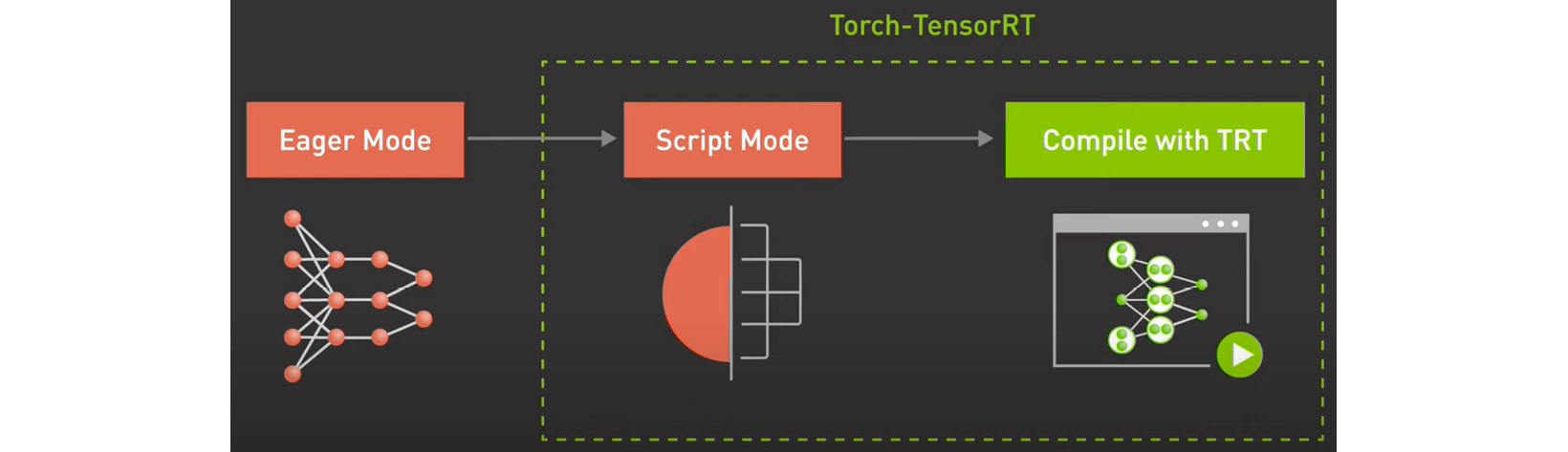
Figure 9.3 – Compiling the PyTorch model using TensorRT-Torch

To compile the PyTorch model using TensorRT-Torch, we need two components:

• A runtime environment for compilation. It’s highly recommended to use NVIDIA’s latest PyTorch containers for this purpose. Note that you will need to run this container on an instance with an NVIDIA GPU available. For instance, you can run this sample on a SageMaker Notebook whose type is g4dn.
• Compilation code. This code will be executed inside the NVIDIA PyTorch Docker container.

Now, let’s review the compilation code:

1. We will start by loading the model from PyTorch Hub, setting it to evaluation mode, and placing it on the GPU device:

   import torch

   import torch_tensorrt

   import os

   torch.hub._validate_not_a_forked_repo = lambda a, b, c: True

   MODEL_NAME = "resnet50"

   MODEL_VERSION = "1"

   device = "cuda" if torch.cuda.is_available() else "cpu"

   # load model

   model = (torch.hub.load("pytorch/vision:v0.10.0", MODEL_NAME, pretrained=True).eval().to(device))

2. Next, we will compile it using the TensorRT-Torch compiler. As part of the compiler configuration, we will specify the expected inputs and target precision. Note that since we plan to use dynamic batching for our model, we will provide several input shapes with different values for the batch dimensions:

   # Compile with Torch TensorRT;

   trt_model = torch_tensorrt.compile(

       model,

       inputs=[

           torch_tensorrt.Input(

               min_shape=(1, 3, 224, 224),

               opt_shape=(8, 3, 224, 224),

               max_shape=(16, 3, 224, 224),

               dtype=torch.float32,

           )

       ],

       enabled_precisions={ torch.float32 },

   )

3. Finally, we will save our model to disk:

   # Save the model

   model_dir = os.path.join(os.getcwd(), "3_src", MODEL_NAME, MODEL_VERSION)

   os.makedirs(model_dir, exist_ok=True)

   print(model_dir)

   torch.jit.save(trt_model, os.path.join(model_dir, "model.pt"))

4. To execute this script, you need to start a Docker container with the docker run --gpus all --ipc=host --ulimit memlock=-1 --ulimit stack=67108864 -it --rm -v $PWD/chapter9/3_src:/workspace/3_src nvcr.io/nvidia/pytorch:22.05-py3 command.
5. Your console session will open inside a container, where you can execute the compilation script by running the python 3_src/compile_tensorrt.py command.

The resulting model.pt file will be available outside of the Docker container in the 3_src directory.

Preparing the model config

Previously, we mentioned that Triton uses a configuration file with a specific convention to define model signatures and runtime configuration. The following code is for a config.pbtxt file that we can use to host the ResNet50 model. Here, we define batching parameters (the max batch size and dynamic batching config), input and output signatures, as well as model copies and the target hardware environment (via the instance_group object):

name: "resnet50"
platform: "pytorch_libtorch"
max_batch_size : 128
input [
  {
    name: "input__0"
    data_type: TYPE_FP32
    dims: [ 3, 224, 224 ]
  }
]
output [
  {
    name: "output__0"
    data_type: TYPE_FP32
    dims: [ 1, 1000 ,1, 1]
  }
]
dynamic_batching {
   preferred_batch_size: 128
   max_queue_delay_microseconds: 1000
 }
instance_group {
  count: 1
  kind: KIND_GPU
}

Refer to the Triton configuration for more details: https://github.com/triton-inference-server/server/blob/main/docs/user_guide/model_configuration.md.

Packaging the model artifacts

To deploy the compiled model with its configuration, we need to bundle everything into a single tar.gz archive and upload it to Amazon S3. The following code shows the directory structure within the model archive:

resnet50
|- 1
  |- model.pt
|- config.pbtxt

Once the model package has been uploaded to Amazon S3, we can deploy our Triton endpoint.

Deploying the Triton endpoint

The Triton inference container is not supported by the SageMaker Python SDK. Hence, we will need to use the boto3 SageMaker client to deploy the model. Follow these steps:

1. First, we need to identify the correct Triton image. Use the following code to find the Triton container URI based on your version of the Triton server (we used 22.05 for both model compilation and serving) and your AWS region:

   account_id_map = {

   # <REDACTED_FOR_BREVITY>

   }

   region = boto3.Session().region_name

   if region not in account_id_map.keys():

       raise("UNSUPPORTED REGION")

   base = "amazonaws.com.cn" if region.startswith("cn-") else "amazonaws.com"

   triton_image_uri = "{account_id}.dkr.ecr.{region}.{base}/sagemaker-tritonserver:22.05-py3".format(

       account_id=account_id_map[region], region=region, base=base)

2. Next, we can create the model, which defines the model data and serving container, as well as other parameters, such as environment variables:

   unique_id = time.strftime("%Y-%m-%d-%H-%M-%S", time.gmtime())

   sm_model_name = "triton-resnet50-" + unique_id

   container = {

       "Image": triton_image_uri,

       "ModelDataUrl": model_data,

       "Environment": {"SAGEMAKER_TRITON_DEFAULT_MODEL_NAME": "resnet50"},

   }

   create_model_response = sm_client.create_model(

       ModelName=sm_model_name, ExecutionRoleArn=role, PrimaryContainer=container

   )

3. After that, we can define the endpoint configuration:

   endpoint_config_name = "triton-resnet50-" + unique_id

   create_endpoint_config_response = sm_client.create_endpoint_config(

       EndpointConfigName=endpoint_config_name,

       ProductionVariants=[

           {

               "InstanceType": "ml.g4dn.4xlarge",

               "InitialVariantWeight": 1,

               "InitialInstanceCount": 1,

               "ModelName": sm_model_name,

               "VariantName": "AllTraffic",

           }

       ],)

4. Now, we are ready to deploy our endpoint:

   endpoint_name = "triton-resnet50-" + unique_id

   create_endpoint_response = sm_client.create_endpoint(

       EndpointName=endpoint_name, EndpointConfigName=endpoint_config_name)

Once the endpoint has been deployed, you can check SageMaker’s endpoint logs to confirm that the Triton server has started and that the model was successfully loaded.

Running inference

To run inference, we must construct a payload according to the model signature defined in config.pbtxt. Take a look at the following inference call. The response will follow a defined output signature as well:

payload = {
    "inputs": [
        {
            "name": "input__0",
            "shape": [1, 3, 224, 224],
            "datatype": "FP32",
            "data": get_sample_image(),
        }
    ]
}
response = runtime_sm_client.invoke_endpoint(   EndpointName=endpoint_name, ContentType="application/octet-stream", Body=json.dumps(payload))
predictions = json.loads(response["Body"].read().decode("utf8"))

This section described the basic functionality of the Triton model server and how to use it on Amazon SageMaker. It’s recommended that you refer to the Triton documentation to learn advanced features and optimization techniques. Keep in mind that depending on your chosen model format and DL framework, your model configuration will be different. You can review the AWS detailed benchmarking for the Triton server for the BERT model at https://aws.amazon.com/blogs/machine-learning/achieve-hyperscale-performance-for-model-serving-using-nvidia-triton-inference-server-on-amazon-sagemaker/. These benchmarks provide a good starting point for experimenting with and tuning Triton-hosted models.

Summary

In this chapter, we discussed how to use popular model servers – TensorFlow Serving, PyTorch TorchServe, and NVIDIA Triton – on Amazon SageMaker. Each model server provides rich functionality to deploy and tune your model inference. The choice of a specific model server may be driven by the DL framework, target hardware and runtime environments, and other preferences. NVIDIA Triton supports multiple model formats, target hardware platforms, and runtimes. At the same time, TensorFlow Serving and TorchServe provide native integration with their respective DL frameworks. Regardless of which model server you choose, to ensure optimal utilization of compute resources and inference performance, it’s recommended to plan how you load test and benchmark your model with various server configurations.

In the next chapter, Chapter 10, Operationalizing Inference Workloads, we will discuss how to move and manage inference workloads in production environments. We will review SageMaker’s capabilities for optimizing your inference workload costs, perform A/B testing, scale in and out endpoint resources based on inference traffic patterns, and advanced deployment patterns such as multi-model and multi-container endpoints.