Numerous experimental measurement techniques depend upon the monitoring of a sensor response as time progresses. Usually an investigator is interested in a change in response; achieving a maximum or minimum signal value; or, in the case of spectroscopic, chromatographic, or electrochemical voltammetry systems, examining the actual shape of the recorded trace.
Although the essence of this chapter is the recording of a sensor response as a function of time, numerous informative data recordings need not be time based, but rather may be recorded as a function of parameters such as frequency, wavelength, temperature, applied pressure, or voltage.
Supervisory control and data acquisition (SCADA) systems such as DAQFactory have been rigorously developed for commercial application to run on Windows operating systems in order to accommodate the large industrial and commercial need for process control. Commercial SCADA programs such as Azeotech DAQFactory and Factory Express are able to offer two-dimensional plotting facilities for x versus y or to display continuous tracings based upon time-stamped data acquisition.
Arduino and the Raspberry Pi have evolved informally in the open source format to fill the constantly changing needs for education, experimental designs, or science-based investigations that may require the rapid prototyping of special- or general-purpose hardware–software combinations. While standardization is virtually an industrial–commercial necessity, it is difficult to realize or implement in a constantly changing “open source” environment where novel technological advances often outweigh legacy compatibility.
The Arduino microcontroller IDE is available in both PC- and RPi-hosted formats. The serial ports on the PC-hosted Arduino are compatible with Microsoft Windows and the DAQFactory program. The RPi-hosted Arduino is compatible with the Linux serial ports and the Python programming language.
The Python realtime data display and recording programs presented in this chapter have been collected from various online and textbook sources then specifically modified to display and record typical Python-derived data or data obtained from interfaced Arduino microcontrollers using the Linux USB-based serial port data-transmission protocols.
Although several of the plotting programs presented are derived from previously published works, the primary intent of this section is to allow the investigator using the Linux-based RPi to develop a simple Python-based, customized plotting facility able to accommodate data from the experimental investigation at hand.
Recalling that a graphic visualization of data can take essentially two forms, consisting of a static or a dynamic display, we should be able to envision that a dynamic display can be created by rapidly displaying a series of slightly differing static images.
Intuitively, the key to minimizing the processing time required to up-date or change the individual static graphic images being displayed is to change only the data that differs between sequential static displays. In order to create a responsive visual display depicting a stream of data coming from a sensor, the individual data points can be stored in an array, and the individual elements of the array can then be positioned sequentially in the screen displays being used to create the dynamic input/sensor-response tracing.
As discussed in previous chapters of this book, graphical displays consume a large amount of computing resources. Complex computing systems often have separate graphics display hardware with very fast dedicated software that is not part of the simpler RPi–Arduino systems.
With limited computing resources available, the graphics displays on the RPi must be relatively simple and optimized for the task at hand. A Python-based graphical strip-chart recorder (SCR) display is literally orders of magnitude slower than the Arduino’s ability to process and stream out data on the serial port.
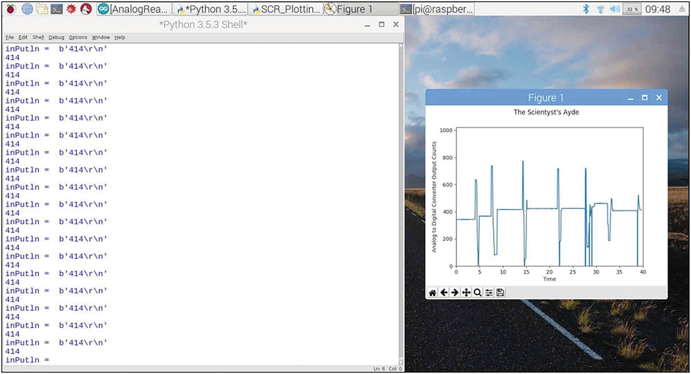
Figure 5-1 is a screen capture of the recording created when the shaft of a 10 kΩ potentiometer connected between 5V and ground is turned, with the wiper voltage wired to the Arduino A0 analog to digital converter (ADC) input. The recording program written in Python is the Matplotlib animation example code: strip_chart_demo.py. The published code, written to emulate an oscilloscope-type response, has been modified to accept data streamed out to the serial port by the Arduino’s ADC. Listing 5-1 (Arduino) and Listing 5-2 (RPi) are able to produce the recording shown in Figure 5-1. (All code listings are provided at the end of the chapter.)
Figure 5-1
Python plot of Arduino ADC output
The Matplotlib program operates by displaying recorded input tracings in timed-width frames. The width of the frames is adjustable, and the correlation between the displayed time units and the actual time of the recording must be determined by the experimenter.
If an actual time base is required for an experiment, the console display can be used to record the current time as the experimental trace for the investigation at hand is displayed. The time-stamped data on the console display can be archived on an SD card if required.
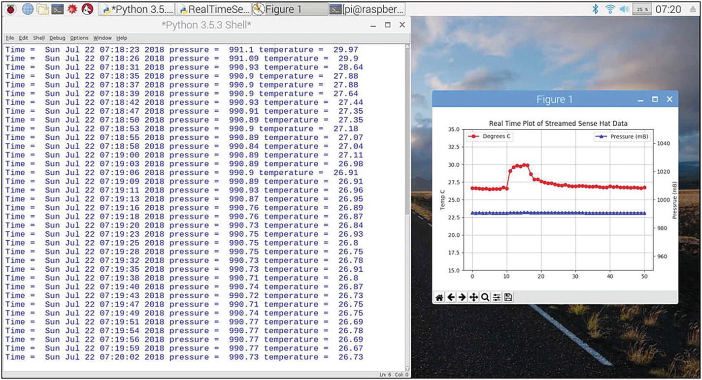
Figure 5-2 depicts a dual-trace display of the temperature and pressure outputs from an RPi Sense HAT board. Listing 5-3 has been written in Python 3 and is based upon the tutorial series presented by P. McWhorter P. Eng.1
Figure 5-2
Python plot of Sense HAT temperature and pressure sensors
The two Python-based graphical display programs presented are relatively easy to use and understand. Both programs have been well documented, are well tested, and are adaptable to the different types of sensor-monitoring applications presented in this book.
/*
AnalogReadSerial
Reads an analog input on pin 0, prints the result to the serial monitor.
Attach the center pin of a potentiometer to pin A0, and the outside pins to +5V and ground.
*/
// the setup routine runs once when you press reset:
void setup() {
// initialize serial communication at 9600 bits per second:
Serial.begin(9600);
}
// the loop routine runs over and over again forever:
void loop() {
// read the input on analog pin 0:
int sensorValue = analogRead(A0);
// print out the value read:
Serial.println(sensorValue);
delay(500); // delay in between reads for stability
}
Listing 5-1
Arduino Code for Transmitting the 0–1023 ADC Values to the Serial Port
# RPi Python Strip-Chart Recorder of Arduino Output
# SCR Plotting of serial data from Arduino output over serial port
# Arduino serial output must be numerical values only and delivered at a rate.
# slow enough for the SCR pgm to plot. i.e., delays of > 250 ms
import matplotlib
import numpy as np
from matplotlib.lines import Line2D
import matplotlib.pyplot as plt
import matplotlib.animation as animation
import time
import serial
#
#
#
class Scope:
def __init__(self, ax, maxt=40, dt=0.02):
"""maxt time width of display"""
self.ax = ax
self.dt = dt
self.maxt = maxt
self.tdata = [0]
self.ydata = [0]
self.line = Line2D(self.tdata, self.ydata)
self.ax.add_line(self.line)
self.ax.set_ylim(0, 1023) # y axis scale
self.ax.set_xlim(0, self.maxt)
def update(self, y):
lastt = self.tdata[-1]
if lastt > self.tdata[0] + self.maxt: # reset the arrays
ax.set_ylabel("Analog to Digital Converter Output Counts")
scope = Scope(ax)
# uses rd_data() as a generator to produce data for the update func, the Arduino ADC
# value is read by the plotting code in 20 or so minute windows for the
# animated
# screen display. Software overhead limits response speed of display.
ani = animation.FuncAnimation(fig, scope.update, rd_data, interval=50,
blit=False)
plt.show()
Listing 5-2
Python Windowed Strip-Chart Recorder with Variable-Width Digit Logic for Serial Port Data Plotting
# Realtime plotting of temperature and pressure from the SenseHat board
import numpy # Import numpy for array manipulation functions
import matplotlib.pyplot as plt #import matplotlib library
from drawnow import * # animation of plotting library
from sense_hat import SenseHat # sense hat library
import time # time stamping data
#
#
sense = SenseHat() # instance of the detector board and sensors
sense.clear() # clear the board
#
#
tempF= [] # list array for temperature data
pressure=[] # list array for pressure data
#
plt.ion() #invoke matplotlib interactive mode to plot live data
cnt=0 # initialize plotter window width counter
def makeFig(): #Create a function to make the plotting window.
plt.ylim(15,35) #Set y min and max values
plt.title('Real Time Plot of Streamed Sense Hat Data') #Plot title
plt.grid(True) #Turn on grid lines of plotter
plt.ylabel('Temp C') #Set ylabel
plt.plot(tempF, 'ro-', label='Degrees C') #plot the temperature in red dots
plt.legend(loc='upper left') #plot the legend
plt2=plt.twinx() #Create a second y axis
plt.ylim(950,1050) #Set limits of second y axis- adjust values as required
plt2.plot(pressure, 'b^-', label='Pressure (mB)') #plot pressure data
plt2.set_ylabel('Pressrue (mB)') #label second y axis
plt2.ticklabel_format(useOffset=False) #Force matplotlib to NOT autoscale y axis
plt2.legend(loc='upper right') #plot the legend
while True:
localtime = time.asctime(time.localtime(time.time())) # time of measurement
pressSH = sense.get_pressure() # collect pressure data
press = round(pressSH,(2)) # round decimal to reasonable value
#
temperature = sense.get_temperature()
temp = round(temperature,(2))
print("Time = ", localtime, "pressure = ", press, "temperature = ", temp) # time stamped data log or record
tempF.append(temp) #Build tempF array by appending temp readings
pressure.append(press) #Build pressure array by appending P readings
drawnow(makeFig) #Call drawnow to update our live graph
plt.pause(.000001) #Pause Briefly. Important to keep drawnow from crashing
cnt=cnt+1 # increment window width counter
if(cnt>50): # at 50 or more points, delete the first one from the array
tempF.pop(0) #This allows us to just see the last 50 data points
pressure.pop(0)
Listing 5-3
Sense HAT Temperature and Pressure Data Plotting and Console Display for Archiving
Summary
Information in experimental data can be contained in the actual numerical values generated by the experiment, in the trace provided by plotting the value as a function of time, or in the shape of a two-dimensional x–y plot of the data.
Programs for plotting one or two streams of sensor data as a function of time are presented and their limitations described.
Chapter 6 describes the concepts of frequency and presents methods and simple equipment for measuring the cycles that determine frequency.