
Everybody loves an Excel trick. I certainly do. I love picking up new shortcuts and secret tips and learning innovative ways of using tools that I never thought to try. We are always learning.
When trying to accomplish an Excel task, sometimes the solution can come from an unexpected source. It could be from a tool that you thought you knew very well. And suddenly a clever new trick has opened your mind to new possibilities. You find yourself eagerly thinking of other ways you can use this new knowledge. I love that feeling.
This chapter will explore some of the tricks that I have learned over the years. I am indebted to my friends, my students, and occasionally my own endeavor in Excel to learning these. I hope these tips become a reference you can refer to again and again.
Fill Techniques
Let us begin with some fill techniques. It is one of the first techniques that you learn in Excel, but there are options that many are not aware of.
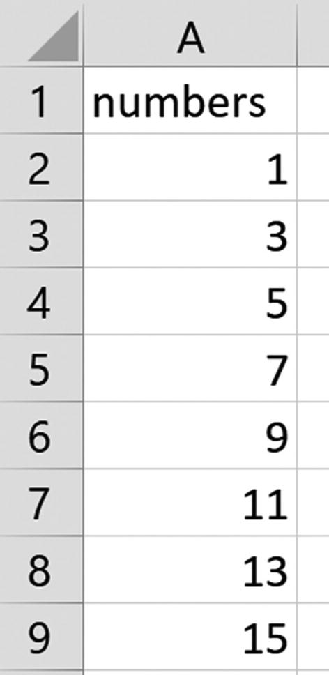
Generate a Number Series
- 1.Enter the first number of the series (1 in this example), select the cell, and position your cursor over the fill handle until you see the skinny black cross. Figure 1-1 shows the fill handle.
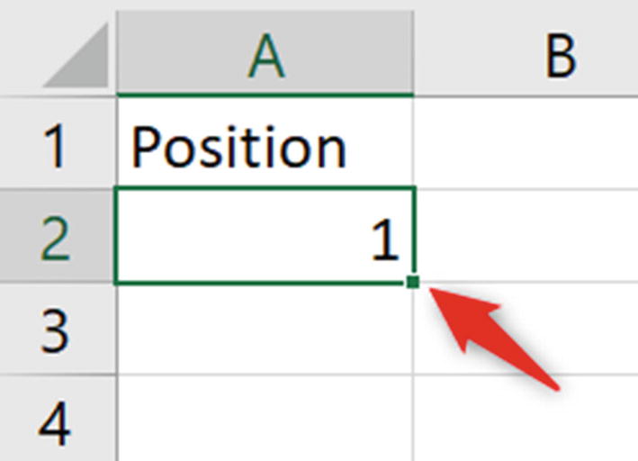 Figure 1-1
Using the fill handle to generate a series of numbers
- 2.
Click and drag down the number of rows you want to generate a number series for.
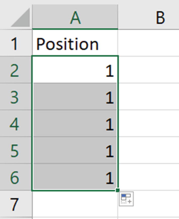
Same number is repeated when you fill down a single number
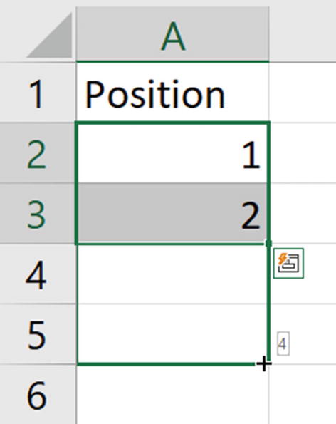
Using two numbers to generate the series
But you do not need to go through that hassle. There are a couple of neat tricks to generate the series. Simply type the first number and hold the Ctrl key down as you fill to generate the sequence.
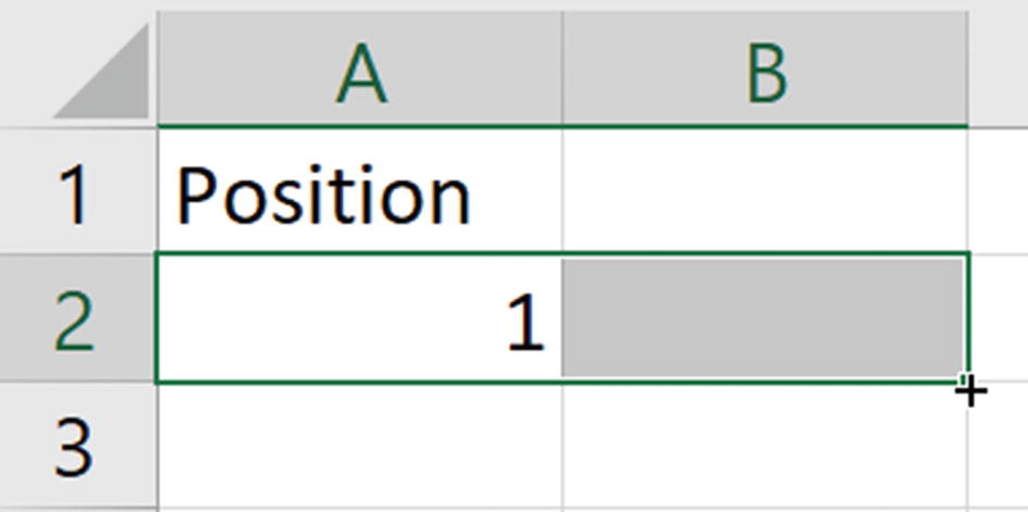
Using the magic square to generate a series of numbers
Additional Series Options
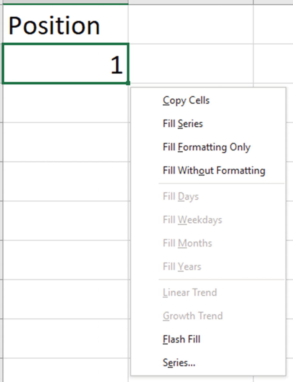
Use the right-click button to drag away and then back to unlock secret options
You can also access these options by clicking Home ➤ Fill ➤ Series.

Additional options in the Series window
In this example, I have set it to step by 2 and to stop at number 15.
This is just one example of what is available. But let us look at a far more realistic scenario.
- 1.
Type 03/03/2020 into the first cell and open the Series window.
- 2.
It should automatically detect that you want to use date values. Ensure this is selected and note the options available for date units.
- 3.
Enter 14 for the Step value and 30/10/2022 for the Stop value. The completed Series window is shown in Figure 1-8.
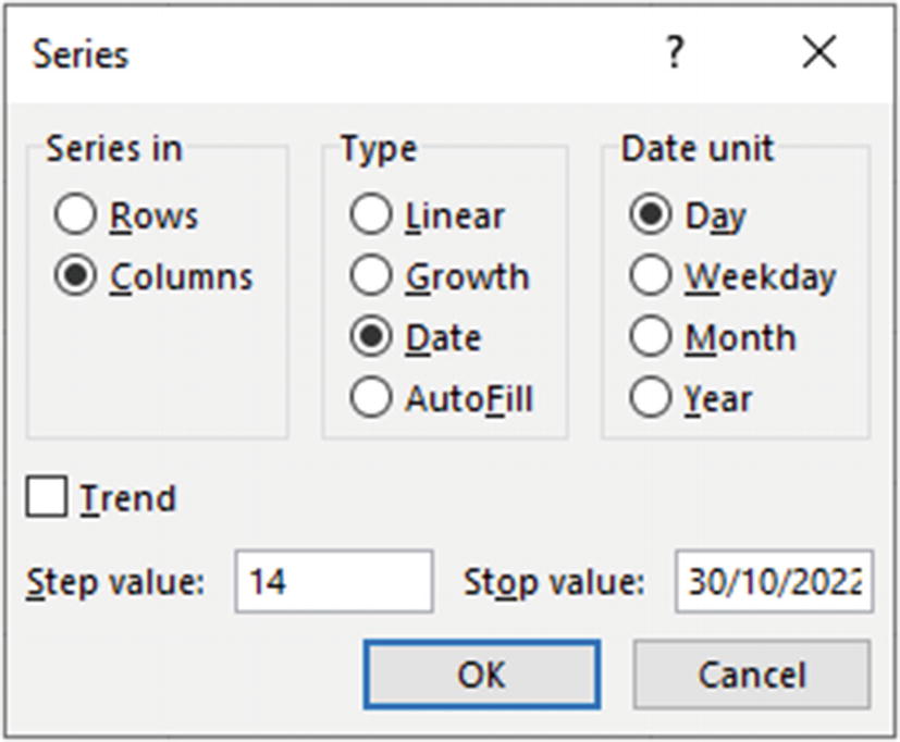
Setting a date series with a stop value
- 4.
Click OK.

Schedule of dates every 14 days from 3 March 2020
In this scenario, the list stops at 25 October 2022 because that is the final Tuesday in the series.
The Incredible Flash Fill
Flash Fill is a tool that arrived with Excel 2013, and the day I first used it, I could not sleep that night. Along with the more important Power Query (Chapter 5), these tools make easy what was once a frustrating task.
Let us look at a couple of examples of what Flash Fill can do and how. These examples just give an insight, and you should further explore what else it can do.
flash-fill.xlsx
For the first example, we have people’s first names in column A and their last names in column B. In column C, we want to combine the two together.
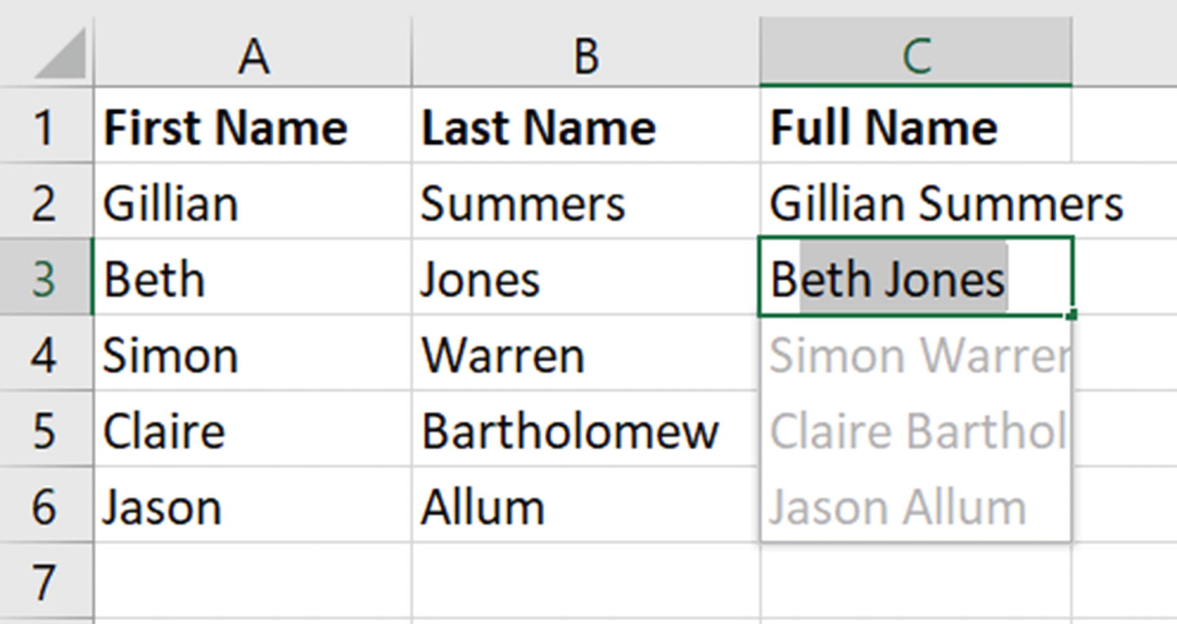
Flash Fill automatically picking up a data entry pattern
So easy to combine hundreds or thousands of names and without any formula.
You can disable this automatic Flash Fill from Excel Options if you do not like this behavior.
For a second example, we have the codes in Figure 1-11, and we want to extract the letters from between the two hyphens (-). They also need to be displayed in uppercase.

A list of codes with information we want to extract
- 1.
Click cell B2 and type “JH”, the first area code in uppercase.
- 2.
Press Ctrl + Enter to confirm your entry but stay on cell B2.
- 3.
Press Ctrl + E. This is the Flash Fill shortcut.
As easy as that, we have the data we want for further analysis (Figure 1-12).
You can also run Flash Fill by clicking Home ➤ Fill ➤ Flash Fill or Data ➤ Flash Fill.

Completed Flash Fill solution for the area codes
Take Advantage of Custom Lists
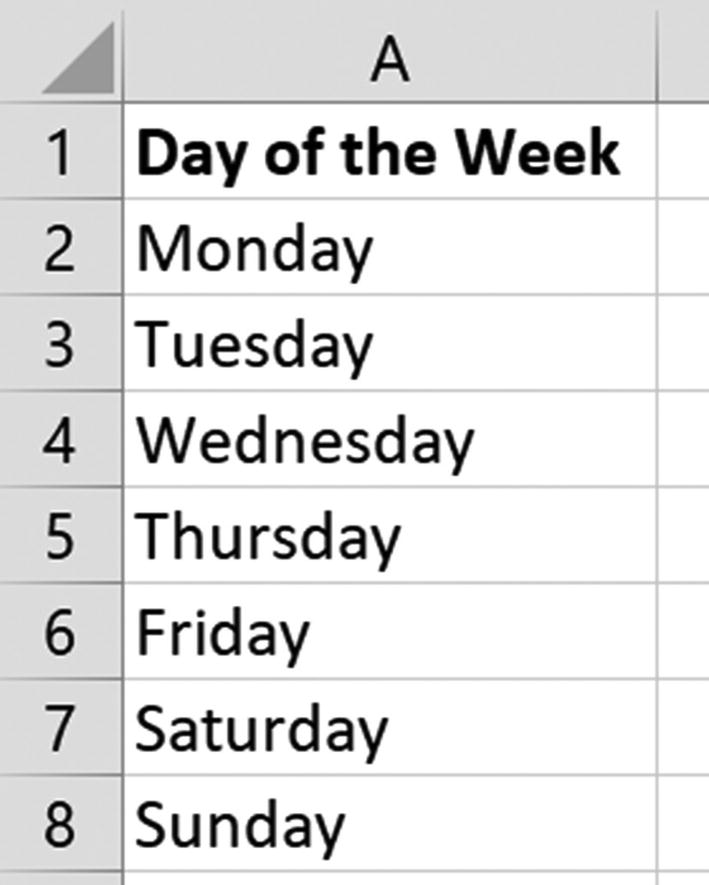
The day of the week series in Excel
You can create your own custom lists in Excel. This can improve the speed and accuracy of entering a series of data. This is very useful.
Another scenario for using custom lists is for sorting data effectively. You can sort lists using a custom list, but what if the items are not in the correct order?
Take this scenario. We have a Slicer connected to a table or PivotTable for filtering. It has the days of the week and is sorted in order (Figure 1-14). But, maybe, for you the first day of the week is not Monday, but Sunday. So, you would prefer this to be at the top when sorted.
custom-lists.xlsx
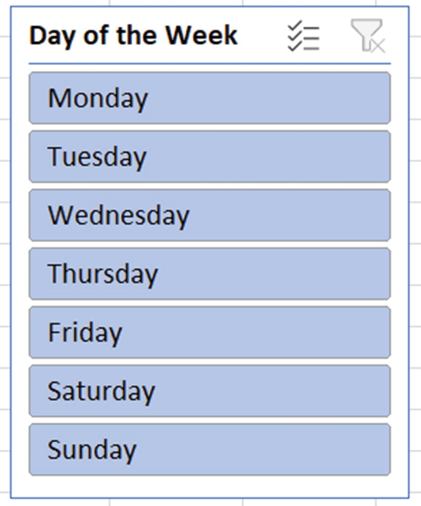
Slicer with the days of the week sorted using the standard custom list
- 1.
Click File ➤ Options ➤ Advanced ➤ Edit Custom Lists (Figure 1-15).

Edit Custom Lists button in the Advanced options
- 2.
You cannot edit the built-in custom lists, so we will need to create a new one. With NEW LIST selected, type the days of the week into the List entries box in the order that you want. Press Enter after each one (Figure 1-16).
- 3.
Click Add to add the new list to the Custom lists on the left, then click OK to close the window.
You can also import a list from a range of cells.

Creating a new day of the week custom list
- 1.
Select the Slicer, then click Slicer ➤ Slicer Settings.
- 2.
Ensure the Use Custom Lists when sorting box is checked (Figure 1-17). You may need to sort it in descending order and then switch back to ascending to get the new custom list to take control.

Use Custom Lists when sorting a Slicer

Slicer sorted using the new custom list
Creating your own version of these month name and day of week custom lists is a typical example. Different scenarios may call for a different “first month.”
You can get creative with this for other work scenarios. Imagine we have many store locations used in a Slicer (or a table or a PivotTable) that we want sorted. But two are our flagship stores (Germany and Switzerland), and we would like to see them at the top of the list for quicker access.
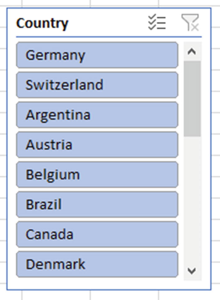
Custom List to specify the order of countries in a Slicer
Change Multiple Worksheets at the Same Time
Occasionally, you may need to make the same change to multiple worksheets at one time. This could be deleting columns, formatting cells, or writing a formula. By grouping worksheets, this task is simple.
group-worksheets.xlsx

The five worksheets and their data

Select all the sheets in a workbook
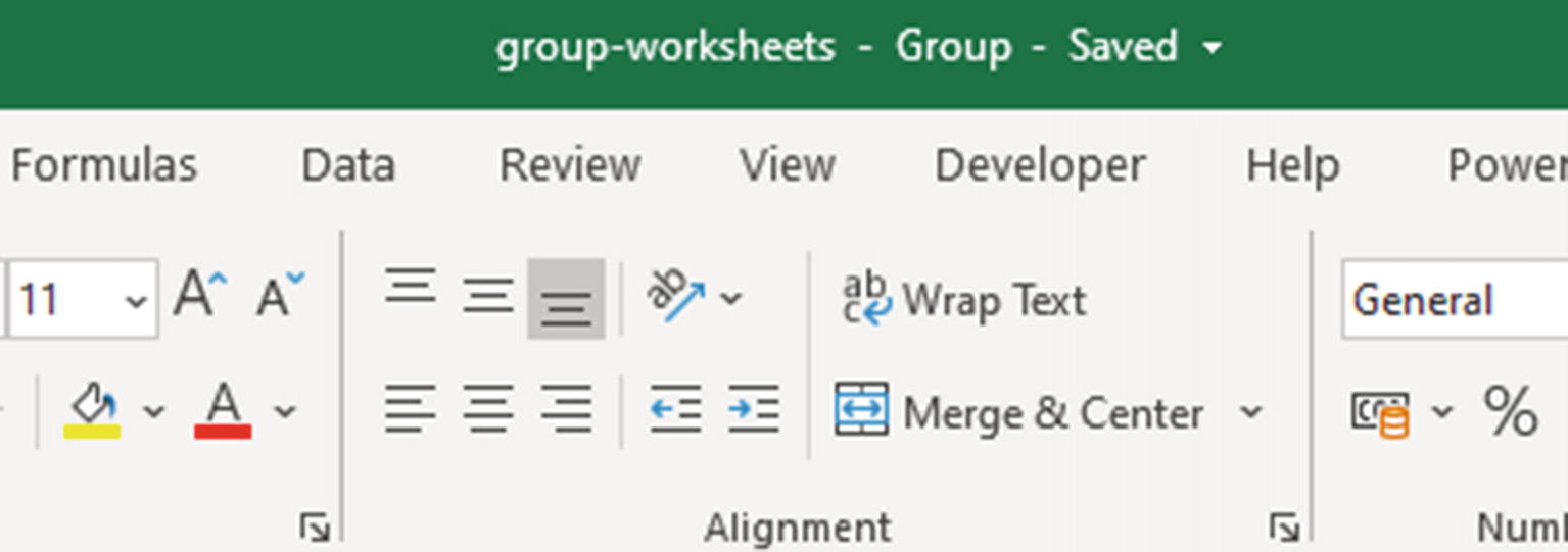
Group in the Excel Title bar
We can now begin to make some changes, and those changes will be replicated on all the sheets.

Formatting and a formula applied to the grouped sheets
To ungroup the sheets, simply click a different sheet tab to the currently active sheet.
You can group specific worksheets by pressing the Ctrl key and clicking each worksheet you would like included in the group. Or to group a consecutive range of worksheets, click the first worksheet, press the Shift key, and click the last worksheet in the range.
Advanced Find and Replace Tricks
Find and Replace is an often-forgotten hero of data manipulation. It has been around for such a long time and is hidden away on the far end of the Home tab of the Ribbon – leading people to forget about it.
Sometimes, these methods are still the best. Fancy formulas, Power Query, and macros are all great. Occasionally though, you just need to get the job done. Here are some examples of when Find and Replace can come to the rescue.
find-and-replace.xlsx
Find and Replace in the Entire Workbook
Let us begin with a huge time saver, being able to replace, format, or remove values from an entire workbook with a few clicks of a button.
We have three worksheets: North East, North West, and South (of course, it could be many more), and we need to make some changes to data across all these sheets.
- 1.
Open the Find and Replace window by using the Ctrl + H keyboard shortcut or clicking Home ➤ Find & Select ➤ Replace.
- 2.
Type “Supreme Pizza” in the Find what box and “Mega Pizza” in the Replace with box.
- 3.
Click the Options button to expand the dialog window.
- 4.
Change the Within setting from Sheet to Workbook. The completed steps are shown in Figure 1-24.
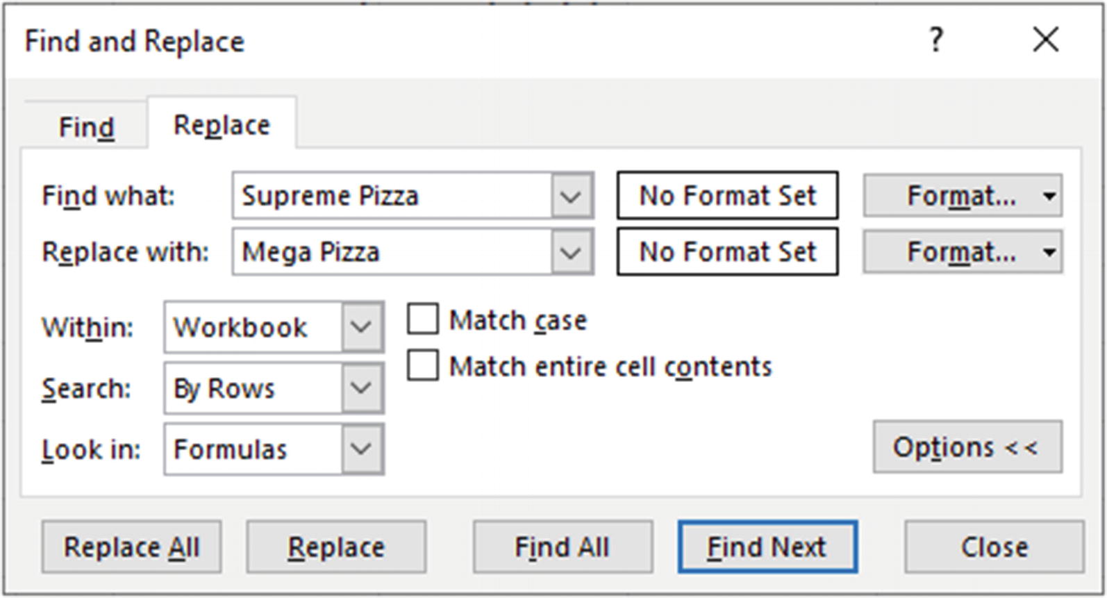
Replace all instances of Supreme Pizza for the entire workbook
- 5.
Click Replace All.

Completion message confirming the number of replacements made
Find and Replace is incredibly powerful, and therefore some care should be taken. The word “Pizza” is included in the search to protect against changing other uses of “Supreme” outside of the one intended.
Edit Your Formulas Fast
The Find and Replace tool is set to look in formulas by default. This setting can be extremely useful for editing many formulas quickly.
They are using sheet references. $C$2:$C$21 refers to the sales values on that sheet.
The ranges on these sheets are now being formatted as tables, and because of these we want to quickly update all formulas to use the table references instead, as this is more efficient.

The NorthEast table with the Sales column
- 1.
Open the Find and Replace window.
- 2.
Enter $C$2:$C$21 in the Find what box and NorthEast[Sales] in the Replace with box.
- 3.
Change the Within setting to Sheet. We need to edit each sheet individually as the tables have different names.
- 4.Ensure that the Look in setting is set to Formulas. The completed steps are shown in Figure 1-27.
 Figure 1-27
Edit all formulas on the worksheet quickly with Find and Replace
- 5.
Click Replace All.
Find and Replace settings are retained. This is useful if you perform that technique regularly on a workbook, but also something to be wary of. Be sure to clear previous settings as you work along with the book examples.
Change Cell Formatting
Yes, it is true. Find and Replace can even be used to locate, replace, or remove based on the cell formatting.
The formulas on the North East, North West, and South worksheets all have a specific formatting applied to them. This is a good idea as it makes the cells containing formulas instantly recognizable to users.
- 1.
Open the Find and Replace window.
- 2.
Click the Options button to make the formatting options available.
- 3.
Next to the Find what box, click the Format button arrow, select Choose Format From Cell (Figure 1-28), and click one of the formula cells.
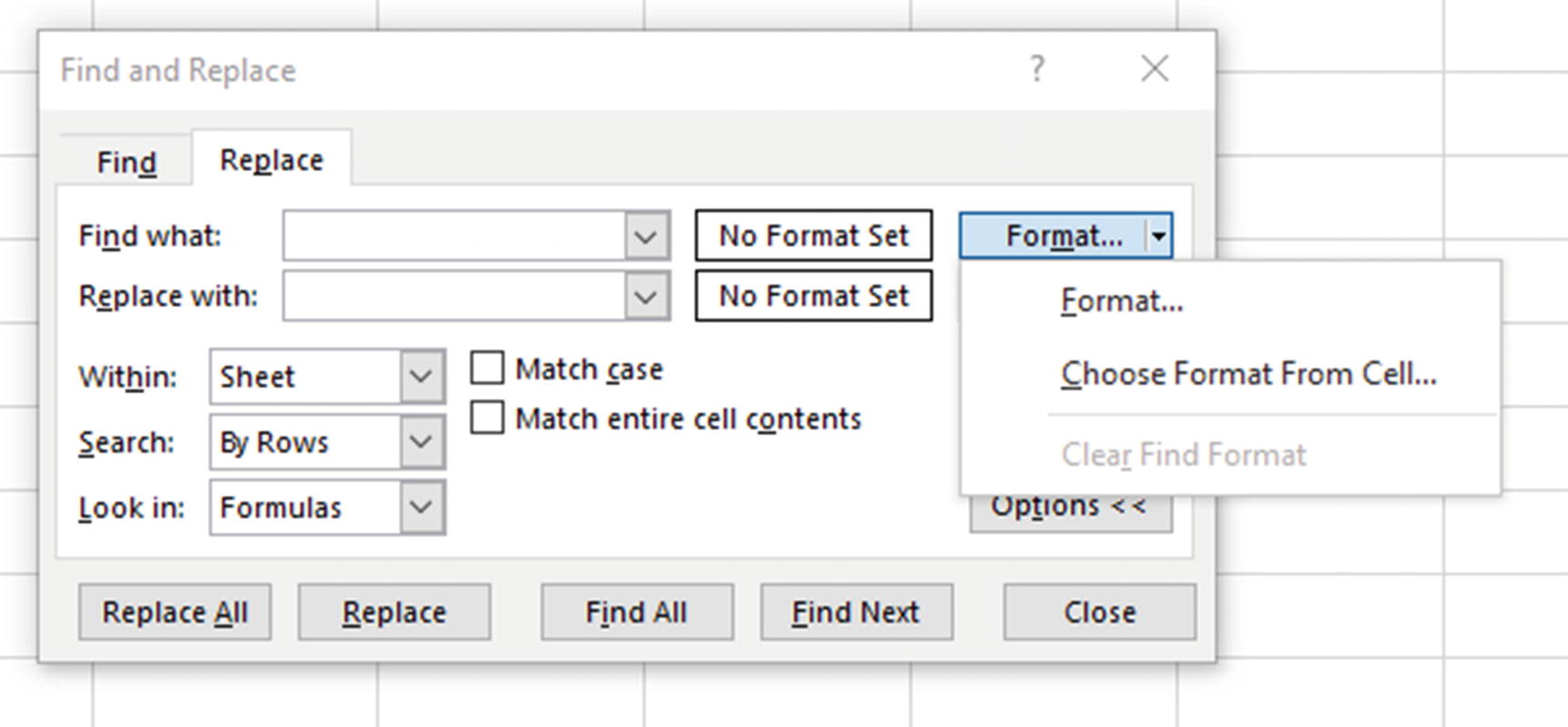
Choose format from a cell
- 4.
Next to the Replace with box, click the Format button arrow and either click Format to specify the formatting to use or Choose Format From Cell if the formatting to use is already applied to a cell.
- 5.Select Workbook from the Within list to change the formatting on all worksheets (Figure 1-29).
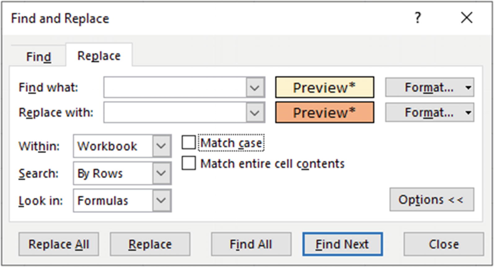 Figure 1-29
Change cell formatting with Find and Replace
- 6.
Click Replace All.
Remove Values
Find and Replace, despite its name, is not only great at finding and replacing values and formatting. But it is also very useful at finding and removing data.

Sample data with total rows that need removing
- 1.
Open the Find and Replace window.
- 2.
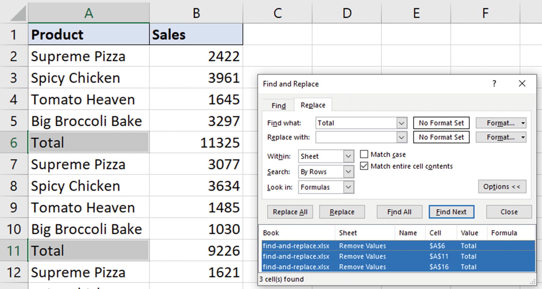
Type “Total” into the Find what box.
- 3.
Select Sheet from the Within list.
- 4.
Click the Match entire cell contents box. We want to be sure that the found cells only contain the word “Total”.
- 5.
Click Find All. A list of all the found cells including information such as the cell address is shown. The completed steps are shown in Figure 1-31.
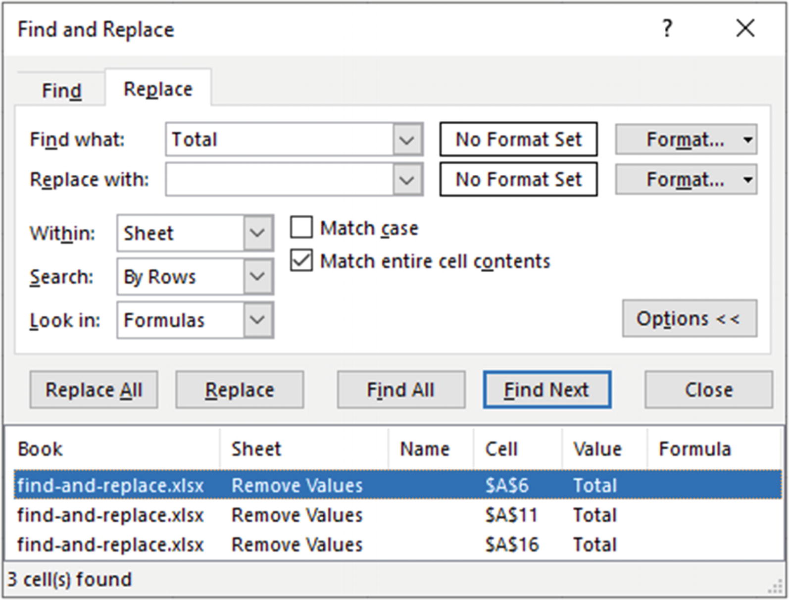
Find all the cells with “Total” as the entire cell content
- 6.
Ensure the area with the list of found cells is active and press Ctrl + A to select all the cells (Figure 1-32).
- 7.
Click Close.
Select all the found cells
- 8.
Click Home ➤ Delete ➤ Delete Sheet Rows to remove the rows that were found (Figure 1-33).

Delete the selected rows on the sheet
Remove Asterisks from a Range
There are two main wildcard characters that can be used in your search criteria. These are the question mark (?) and the asterisk (*).
These wildcard characters can be used in place of characters you are unsure of. The question mark can be used in place of a single character. For example, A?an would find both Adam and Alan. And the asterisk can be used in place of any number of characters. For example, L*n would find both London and Linton.
If the asterisk and question mark are wildcards, how would you look for those characters specifically if needed?

List of imported names including asterisk characters

Using the tilde to find the asterisk characters
The tilde informs the Find and Replace tool that the following character should be used as the search criteria and not as a wildcard.
This can also be used to replace or remove the question mark. If you need to replace or remove a tilde, use two tildes (~~) in the Find what box.
Replace Line Breaks Easily
Line breaks are another type of nasty character that you can find yourself removing from Excel spreadsheets, especially when you are getting data from external sources. Once again, though, this is easy with Find and Replace.
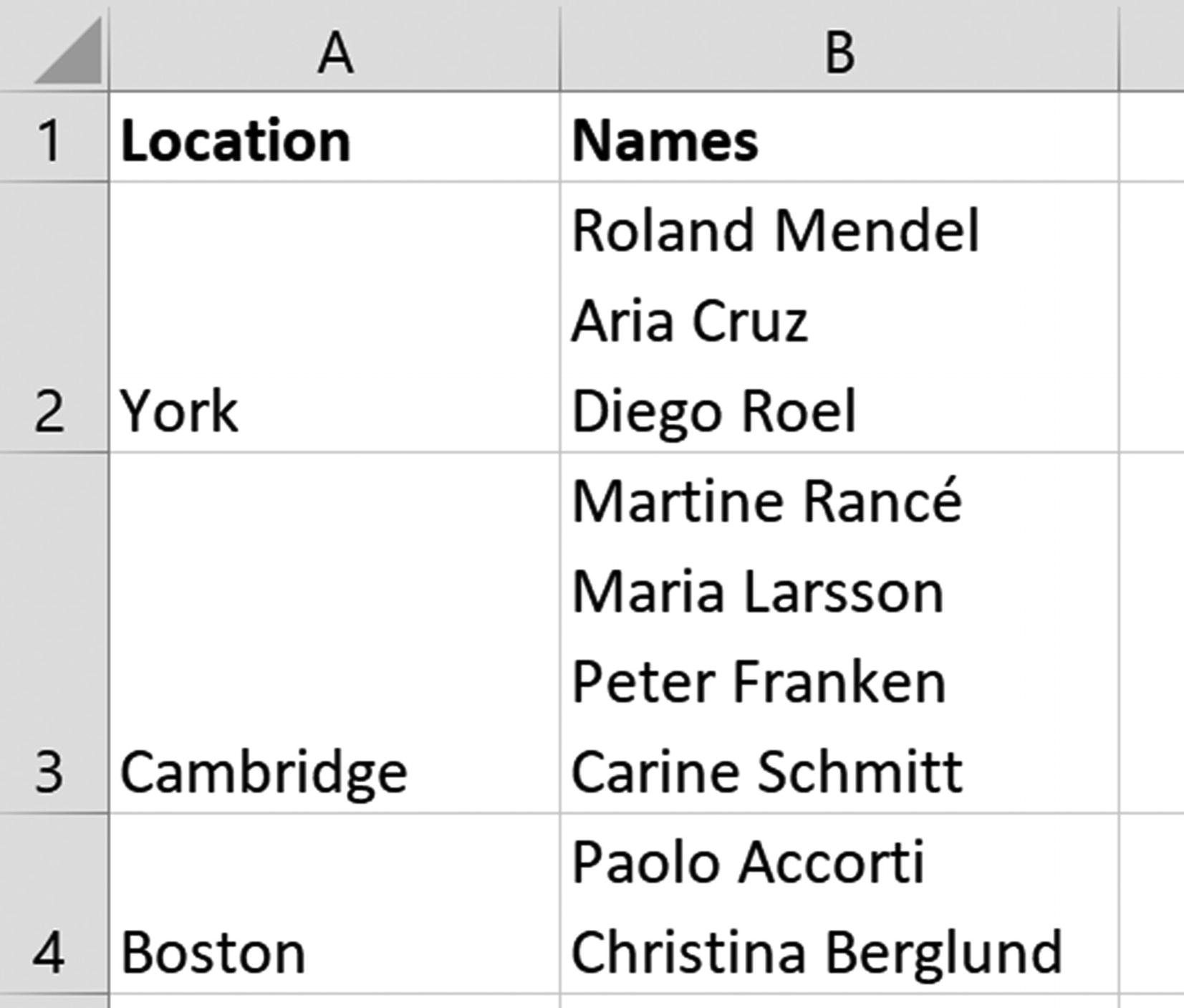
Line breaks separate the names in column B
- 1.
Select the range of names and open the Find and Replace window.
- 2.
In the Find what box, press Ctrl + J on the keyboard. This shortcut inserts a line break for the search criteria (it may not be visible).
- 3.
In the Replace with box, type a comma and a space (, ) (Figure 1-37).
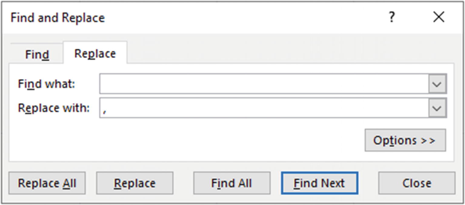
Replace line breaks with Find and Replace
- 4.
Click Replace All to replace all the line breaks.
- 5.
Click the Wrap Text button on the Home tab to remove the text wrapping enforced by the line breaks.
The line break is character 10 on Windows and 13 on a Mac. You can also replace the line breaks using the CHAR function with the appropriate character code within the SUBSTITUTE function if you wanted a formula solution.
Delete Every Nth Row Quickly
At times we need to be inventive, and if we cannot search directly for the text we need, a helper column can be created.
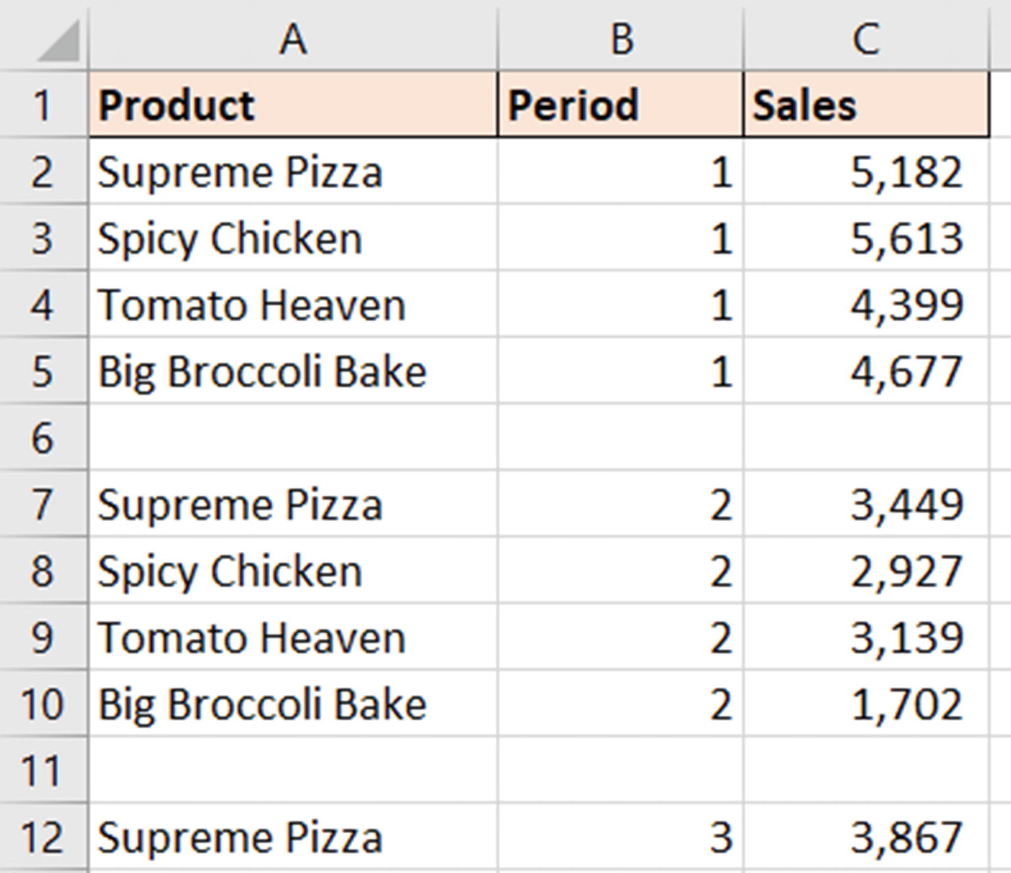
In this example, we have a list of sales data with total rows inserted into the range which we want to remove. The total rows are labeled with the region name so we do not have consistent text that we can use as search criteria, but they do occur in every fifth row.
- 1.
In column C, type the characters into the first five cells. You can use any characters you want; just ensure that the one in the fifth row is unique.
- 2.
Select these five cells and fill the list to the bottom of the range to generate the series of characters. You can do this quickly by double-clicking the fill handle.
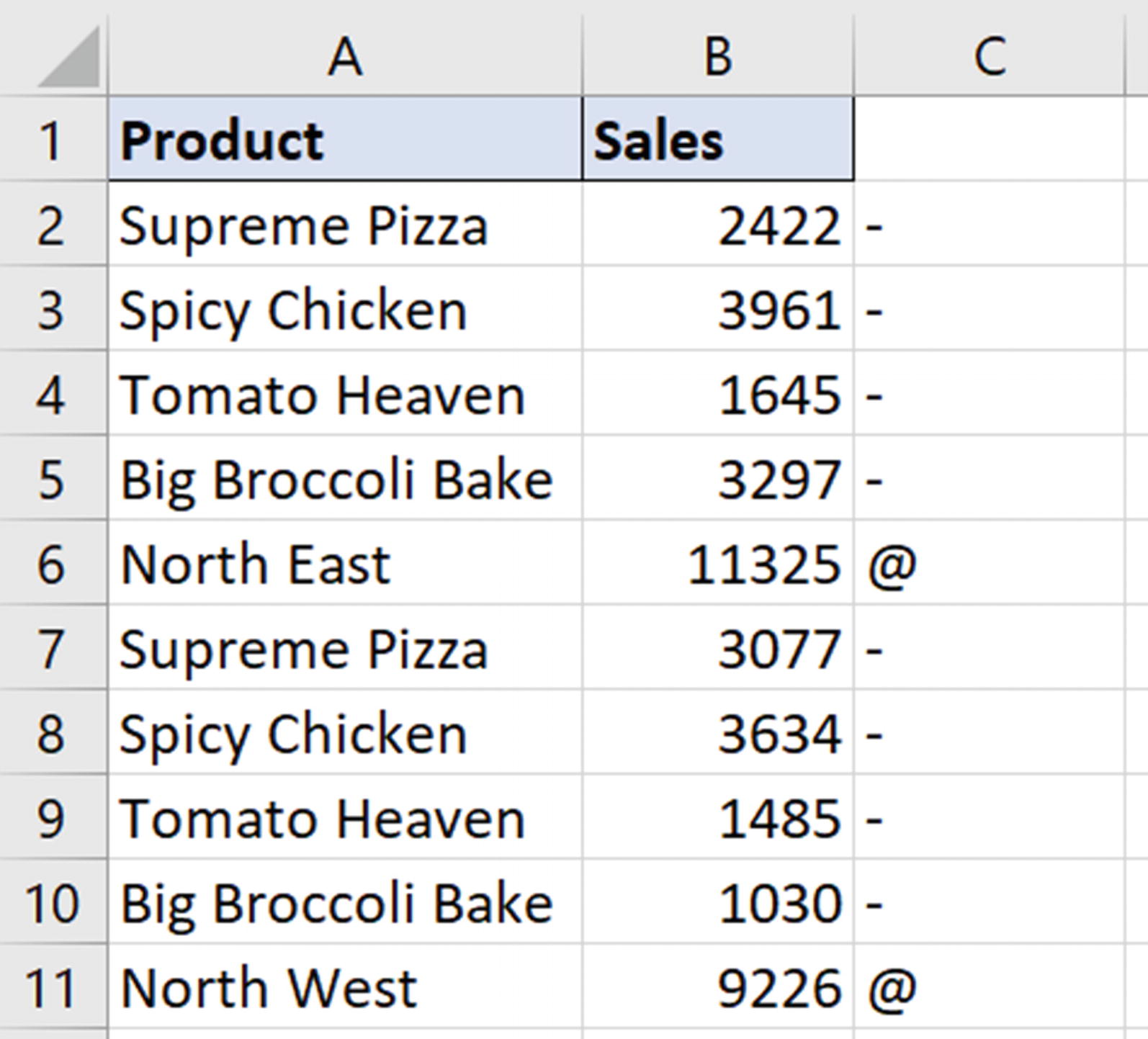
Generate a series of characters to identify the rows we need
- 3.
In the Find and Replace window, type the unique character in the Find what box. Click Find All to list the cells containing that character.
- 4.
Press Ctrl + A to select all the cells (Figure 1-39).
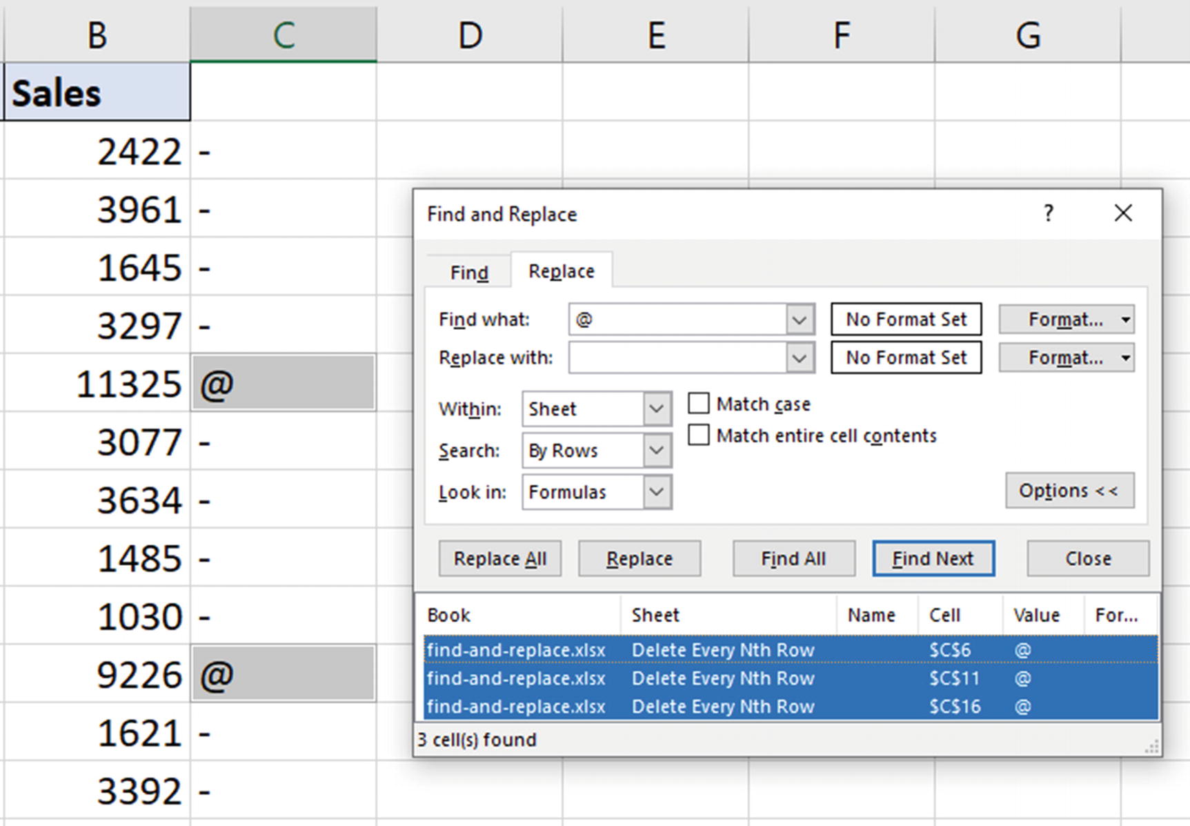
Select all the cells with that unique character
- 5.
Click Home ➤ Delete ➤ Delete Sheet Rows to remove every fifth row.
Quickly Find All Cells That Meet Criteria
The Go To Special tool is incredibly useful and enables us to select all cells that meet specific criteria easily. It is fantastic for auditing spreadsheets and performing quick no-nonsense tasks.
go-to-special.xlsx
Remove Blank Rows
The problem of blank rows is an unfortunate tale that all Excel users experience at some point. The good news is that the shining knight of Go To Special will help rid them from our spreadsheets.
Go To Special provides a quick and no fluff way of getting the job done. In Chapter 5, we cover Power Query which can handle this task more efficiently and do much more.
Blank rows in a spreadsheet. Bad news!
- 1.
Select the range to search for blanks. In this example, I will select column A as that is sufficient to identify a blank row.
- 2.
Press F5 to open the Go To window and click Special, or click Home ➤ Find & Select ➤ Go To Special to open the Go To Special window.
- 3.
Select Blanks (Figure 1-41) and click OK.
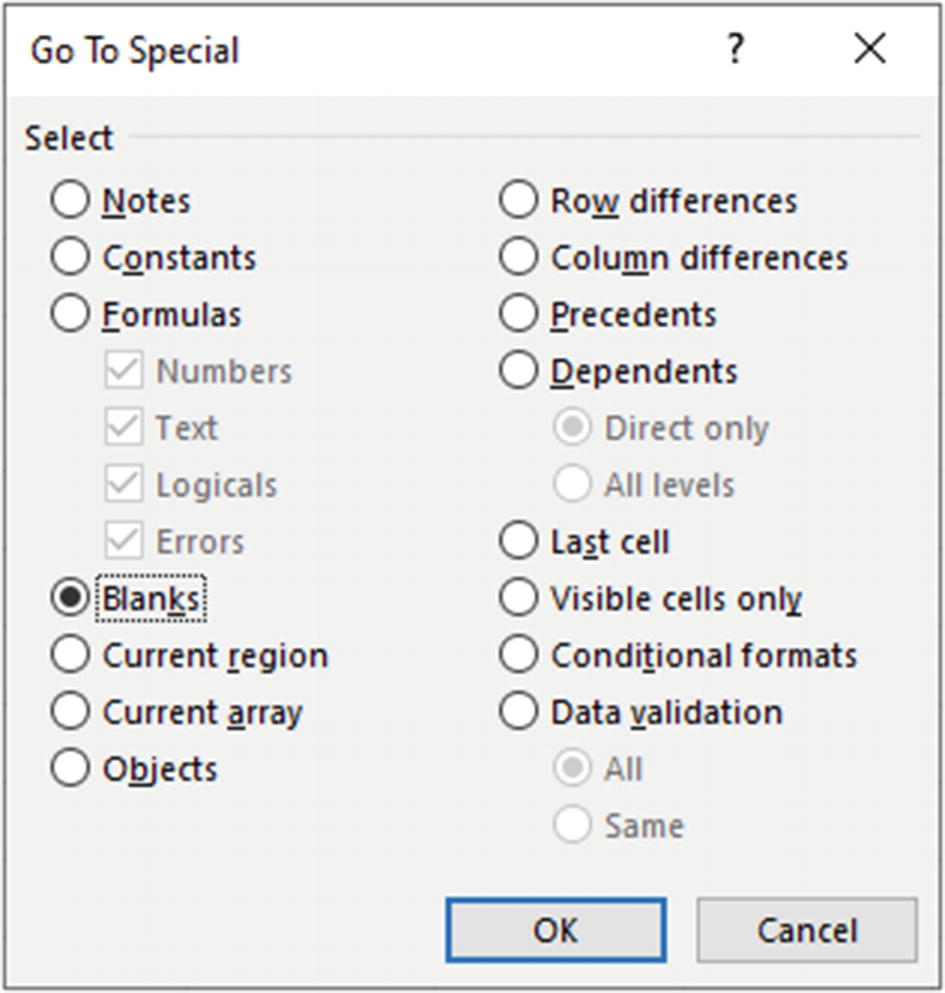
Select Blanks in the Go To Special window
- 4.
Click Home ➤ Delete ➤ Delete Sheet Rows.
To open the Go To Special window, you can use either the F5 or Ctrl + G shortcuts followed by Alt + S.
Fill Blank Cells with 0
In addition to blank rows to remove, there is the other common issue of blank cells.
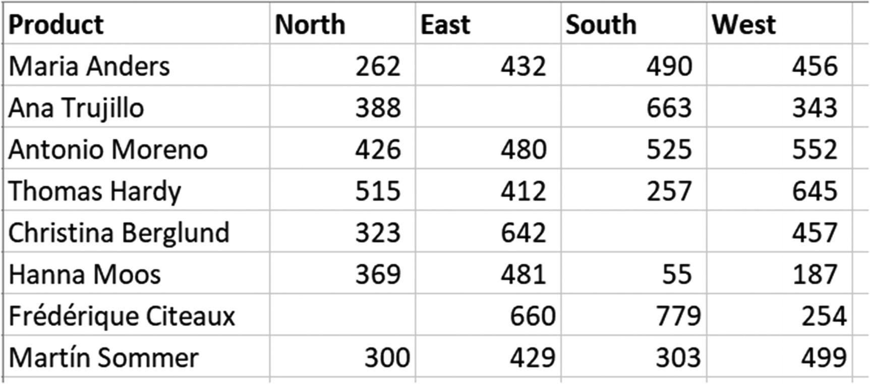
Blank cells in a data set
- 1.
Select the range containing the blanks to fill. In this example, I will select columns B:E.
- 2.
Click Home ➤ Find & Select ➤ Go To Special, select Blanks, and click OK.
- 3.
All the blank cells in the range are selected. The first one is the active cell (Figure 1-43).
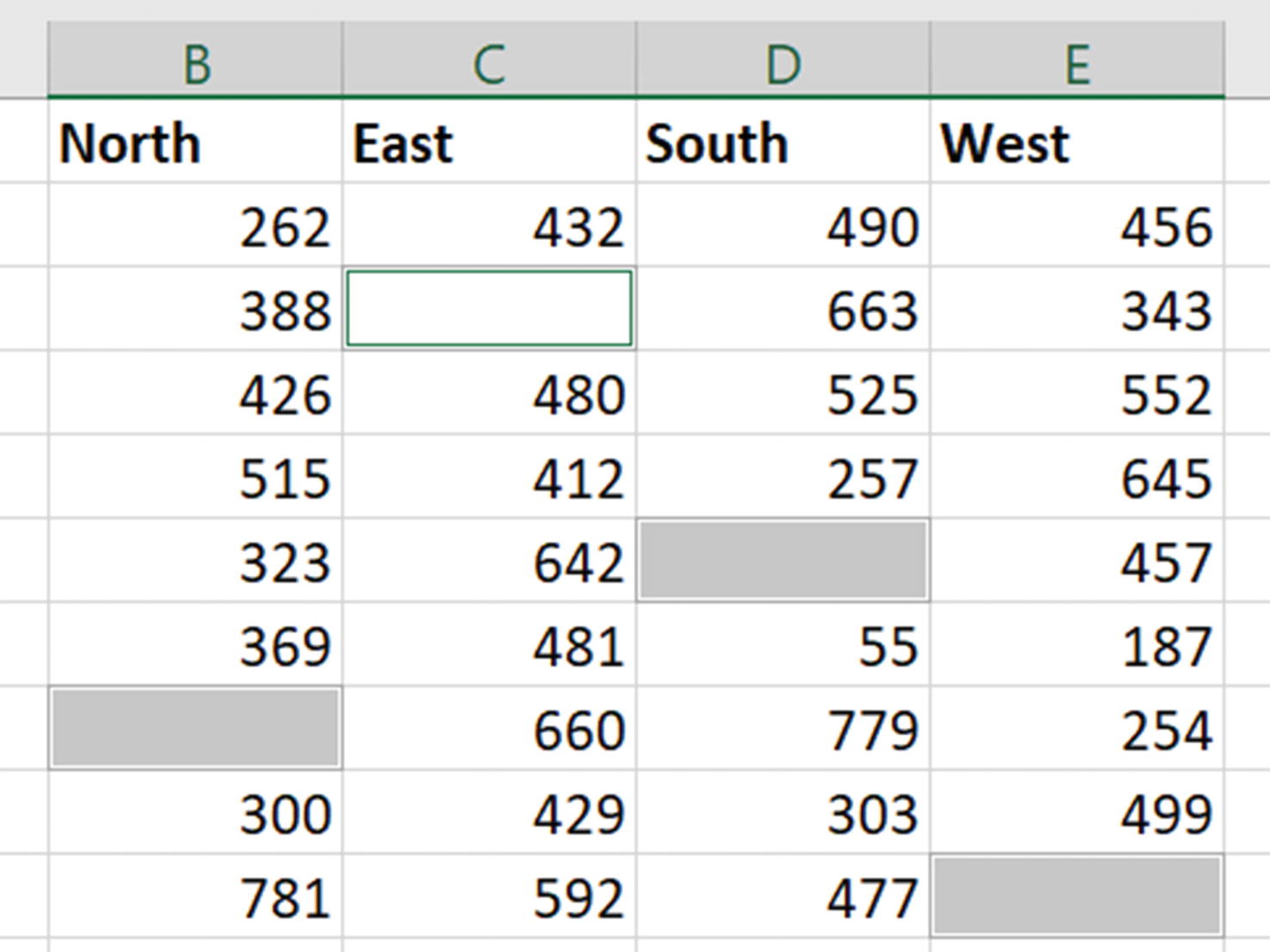
Quickly select all the blank cells in a range
- 4.
Type 0. This will appear in the active cell only. Press Ctrl + Enter to apply to all the other selected cells (Figure 1-44).
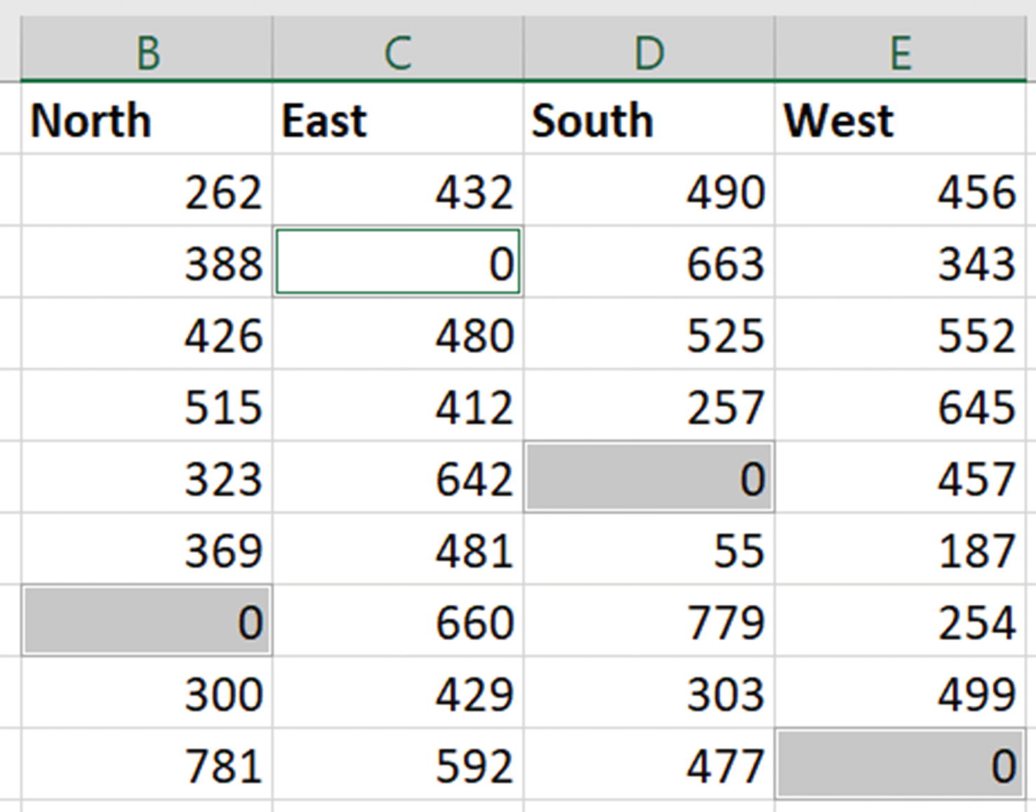
Zero in all blank cells
Fill Blank Cells with the Cell Value Above
Exporting reports from other systems into Excel often leaves us with data that is awkward to analyze further. Take the example in Figure 1-45 which has blank cells under the labels in the first two columns.
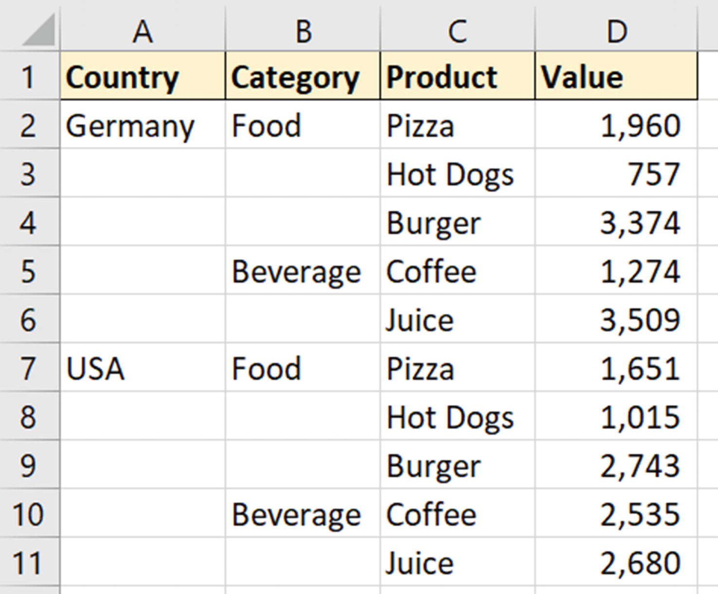
Exported report containing blank cells
- 1.
Select the range containing the blanks to fill. In this example, I will select columns A:B.
- 2.
Click Home ➤ Find & Select ➤ Go To Special, select Blanks, and click OK.
- 3.
The blank cells are selected. Type = and click the cell above the active cell. In Figure 1-46, that is cell B2.
- 4.
Press Ctrl + Enter.

Fill the blanks with the value from the cell above
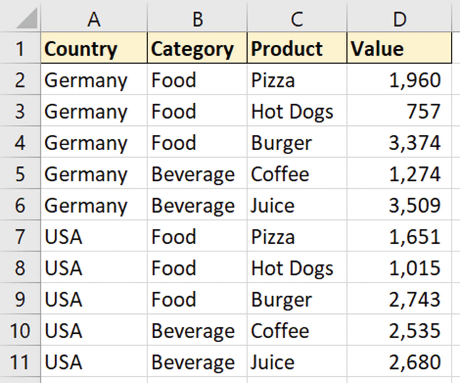
Completed Excel range with blanks filled from the cell value above
Format All Cells Containing Formulas
When creating models and reports in Excel, it can be awkward to remember which cells contain input values or which contain formulas.
Doing something simple such as formatting these cells differently will give them that distinction so that it is no longer a headache in the future.
- 1.
Open the Go To Special window.
- 2.
Click the Formulas option. You can be more specific and select the formulas that return numbers, text, logicals, or errors, if needed. We will select all (Figure 1-48).
- 3.
With the formulas selected, they can now be formatted how you want.

The formulas options in the Go To Special window
Compare Two Columns by Identifying Row Differences
When auditing spreadsheets, you may need to highlight inconsistencies between values in different columns. Go To Special has an option to quickly identify these differences.

Data with columns to compare
- 1.
Select the range of cells to compare. In this example, this is B2:C6.
- 2.
Open the Go To Special window by pressing F5 followed by Alt + S, or click Home ➤ Find & Select ➤ Go To Special.
- 3.
Click the Row differences option (Figure 1-50) and click OK.

Row differences option in the Go To Special window

Formatting applied to identify the row differences
The Secrets of Text to Columns
The Text to Columns feature is very well known in Excel, but it does have some secret abilities that you may not be aware of.
text-to-columns.xlsx
Convert Text to Number
Text to Columns is one of the fastest no-nonsense ways to convert data. Many users do not realize this because its name implies that it will split data into columns. But you do not have to.
- 1.
Select the range of text you want to convert to numbers.
- 2.
Click Data ➤ Text to Columns to open the Text to Columns wizard.
- 3.
Leave the first step as Delimited and click Next.
- 4.
Remove all delimiter options in step 2. We are not interested in splitting columns. Click Next.
- 5.
Ensure General is selected as the format (Figure 1-52). This will convert numbers and dates if it recognizes them. Click Finish.
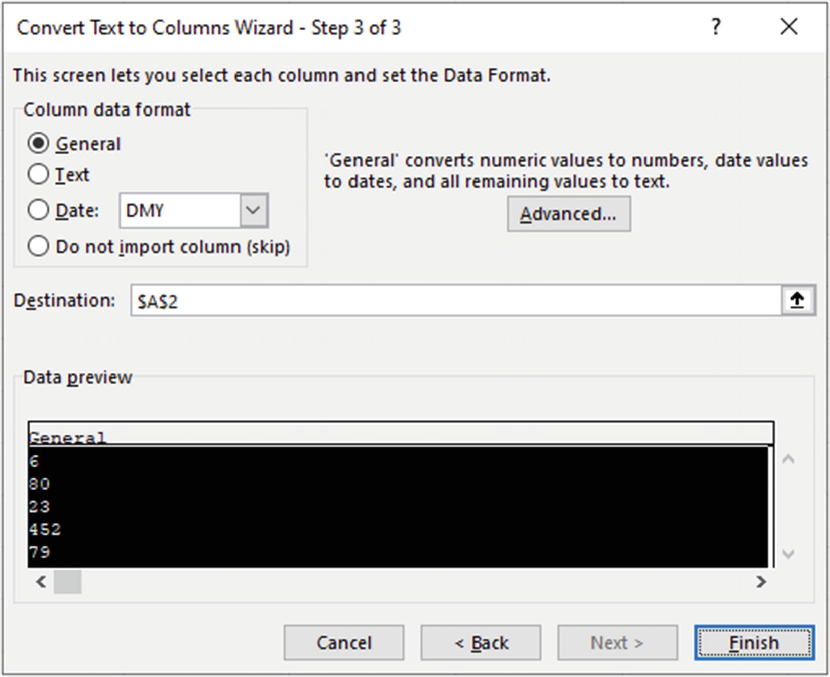
Convert text to numbers with Text to Columns
Converting Date Formats
Excel can sometimes have trouble recognizing dates. This could be that they have come from a country with a different format to the regional settings of your Excel. For example, I am based in the UK, so dates formatted as MM/DD/YYYY are not recognized as a date.
Figure 1-53 shows dates in the MM/DD/YYYY formats. Two of the dates are stored as text, and two have been stored as dates. Excel thinks it understands two of them, but the dates are wrong as they do not follow the expected DD/MM/YYYY format.

Dates in MM/DD/YYYY not recognized by my Excel
- 1.
Select the range of dates and click Data ➤ Text to Columns.
- 2.
Leave the first step as delimited, and ensure no delimiters are used in the second step.
- 3.
On step 3, click the Date option and select MDY from the format list (Figure 1-54). Click Finish.

Select the format that the dates are using
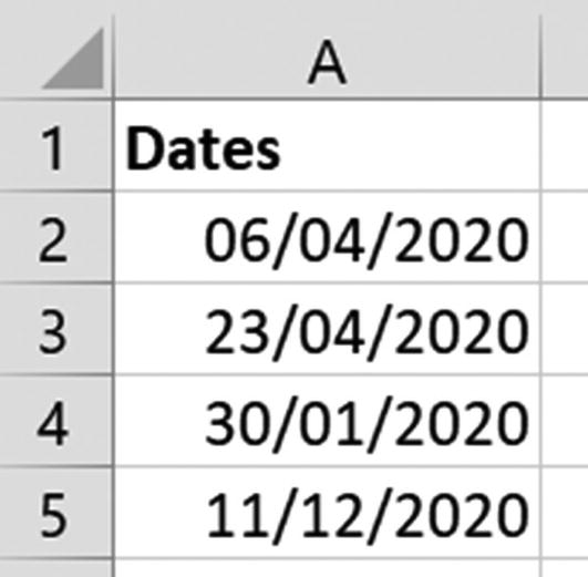
MM/DD/YYYY dates successfully converted to DD/MM/YYYY
Text to Columns can be used to convert from any date format. This could be dates stored as text or dates using a YYYYMMDD format.
It is one of my favorite secrets about the feature. And when I use it to resurrect thousands of unrecognized dates in a few seconds, it always impresses.
Converting International Number Formats
It is also a quick way of handling international number formats. I live in the UK, so the comma (,) is used as a thousand separator and the period (.) as a decimal separator.
Not all countries use the same characters so there can be confusion in Excel when working with data from other countries. Figure 1-56 shows numbers that use a comma (,) as the decimal separator and the period (.) as the thousand separator. My version of Excel does not recognize these as numbers, though it did recognize the 9.

International numbers not recognized by Excel
- 1.
Select the range of numbers to convert and click Data ➤ Text to Columns.
- 2.
Leave the first step as delimited, and ensure no delimiters are used in the second step.
- 3.
In step 3, click the Advanced button.
- 4.
Change the Decimal separator and the Thousands separator to the ones used by the data (Figure 1-57).

Advanced settings for converting text to numbers
- 5.
Click OK to close the advanced settings and then Finish.
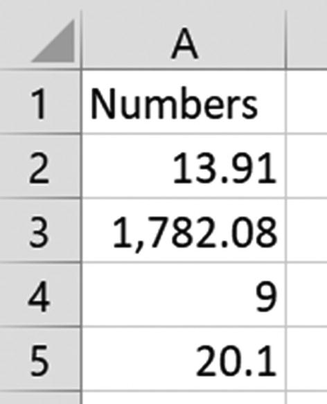
International numbers successfully converted
Convert Values with a Trailing Minus Sign
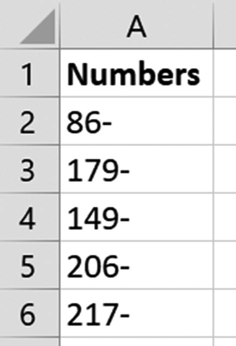
Numbers with a trailing minus sign
- 1.
Select the range you need to convert and click Data ➤ Text to Columns.
- 2.
Leave the first step as delimited, and ensure no delimiters are used in the second step.
- 3.
In step 3, click the Advanced button and check that the Trailing minus for negative numbers box is checked (Figure 1-60). By default, it should be so this is an often unnecessary check.

Trailing minus for negative numbers check box in advanced settings
- 4.
Click OK and then Finish.

Text values converted to negative number values
What Is So Special About Paste Special?
Paste Special is an incredible tool for quickly manipulating data. It is very helpful for simple but brilliant time-saving data formatting and other transformations.
paste-special.xlsx
Convert Positive Values to Negative
- 1.
Type -1 into a vacant cell.
- 2.
Copy that cell value by pressing Ctrl + C.
- 3.
Select the range of cells you want to convert and click Home ➤ Paste arrow ➤ Paste Special or use the Ctrl + Alt + V shortcut.
- 4.
In the Paste Special window, select Values and Multiply (Figure 1-62).
Multiplying the values by –1 converts them to negative. The same technique converts negative values to positive.
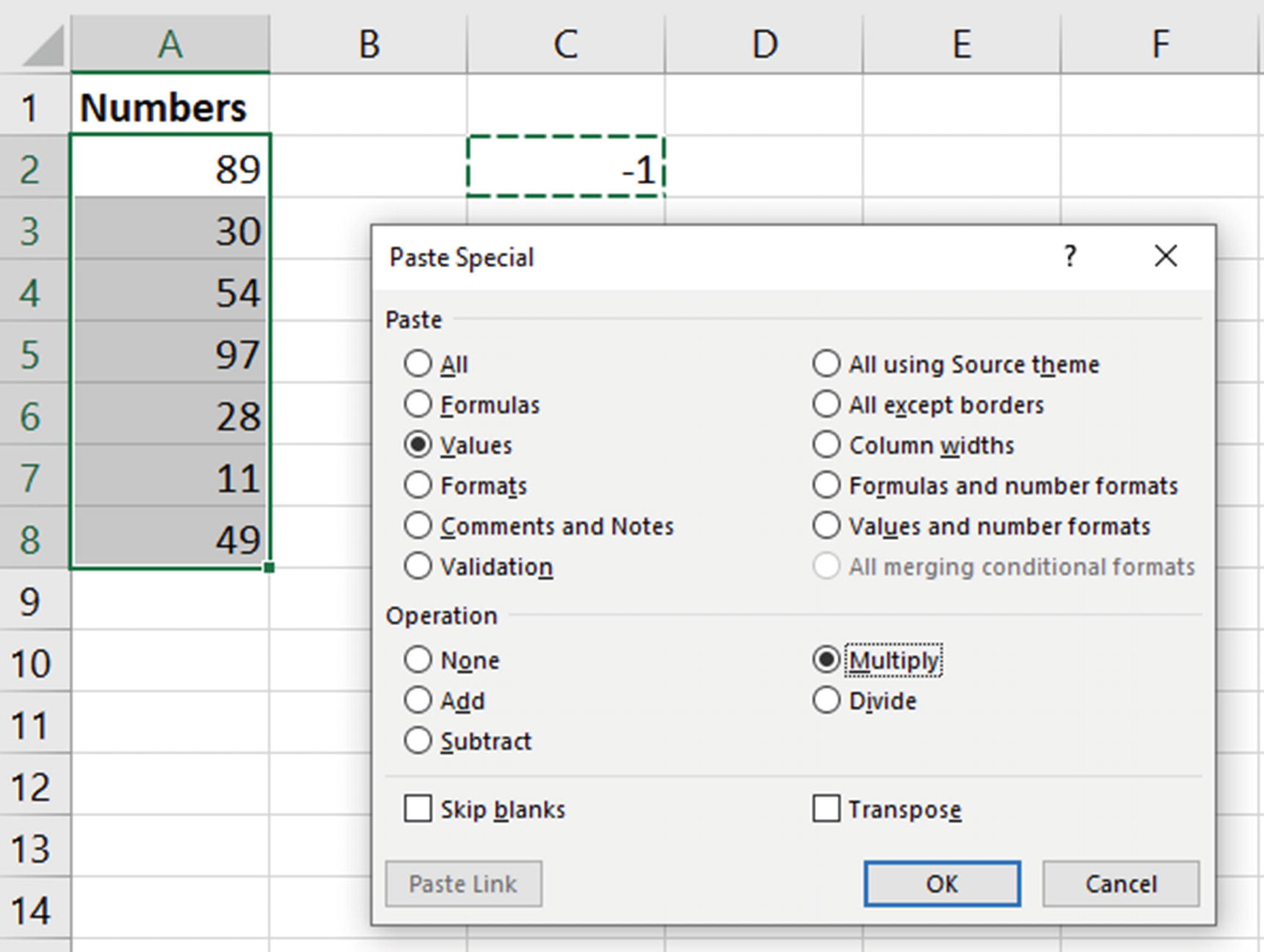
Convert positive numbers to negative with Paste Special
Remove Formulas from a Cell
Pasting values only to remove the formulas from a cell is probably the most common use of Paste Special.
- 1.
Select the range containing the formulas you want to replace with values only.
- 2.
Position your cursor on the edge of the selected range, right-click and drag away from the selection, then back again and release the mouse.
- 3.
A menu appears with some useful paste options (Figure 1-63). Click Copy Here as Values Only.
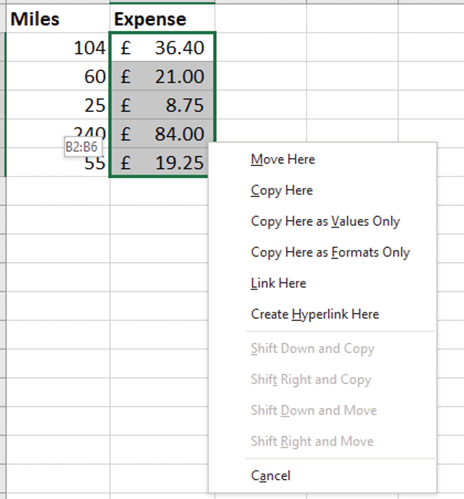
Right-click wiggle to paste as values only
Repeat Column Widths
This is a question I get a lot on my beginner’s classes in Excel. How can we make each column the same width quickly?
Figure 1-64 shows four columns, and the “Qtr3” column is clearly wider than the other three. Also, how do we know the other three are the same width?

Column C is wider than the other three columns
- 1.
Click a cell in column A (“Qtr1” column) and press Ctrl + C to copy.
- 2.
Select cells in columns B:D. Just some cells in all three columns is enough; you do not need to select the entire column.
- 3.
Press Ctrl + Alt + V to open the Paste Special options.
- 4.
Select Column Widths and click OK.
Pasting with Charts
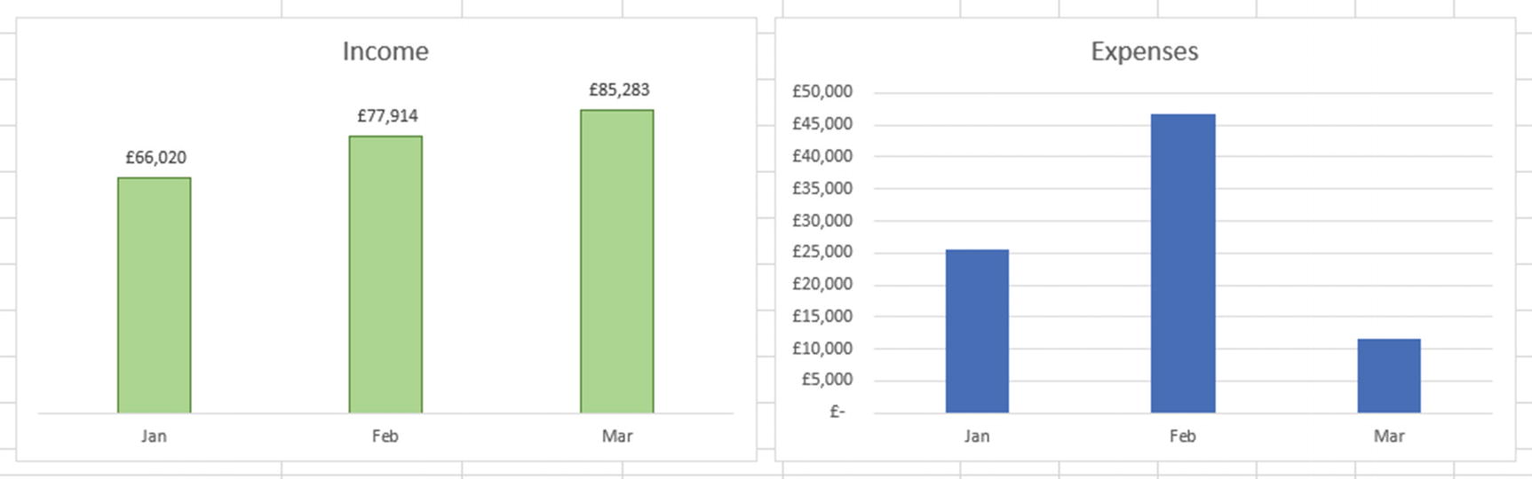
Two charts with different formatting
- 1.
Select the chart with the format you want to copy and press Ctrl + C.
- 2.
Click the chart you want to paste the formatting to.
- 3.
Click Home ➤ Paste arrow ➤ Paste Special to open the window shown in Figure 1-66.

Paste Special options for charts
- 4.
Select Formats. We do not want to paste the data as well.

Same formatting applied quickly between two charts