
Power Query is one of the most important updates in the history of Excel. What once seemed impossible or would require VBA is now very simple. Understanding the role of Power Query will change the way you work with data.
This chapter will walk through several examples of how you can use Power Query to streamline tasks and prepare data for analysis. Be ready! You will never work the same way again.
Introduction to Power Query
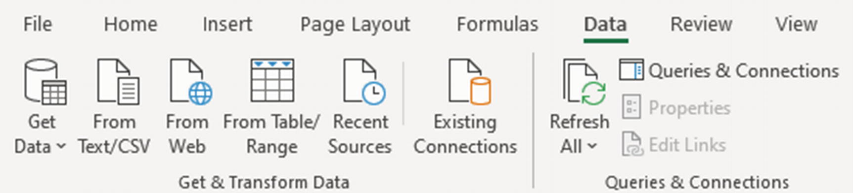
Get & Transform on the Data tab
Microsoft is regularly making improvements and releasing updates to Power Query, so Microsoft 365 users will always have the latest features available.
The role of Power Query is to import, clean, and prepare data for analysis.
Excel in the past was limited in how we got external data into Excel. We relied on the external software or website having good export to Excel functionality.
Once in Excel, we then used formulas and features such as Text to Columns, Filter, Remove Duplicates, and Find and Replace to transform it. This was frustrating and took time.
Power Query fills in this gap. And better yet, it has a nice easy-to-use interface with buttons that many Excel users will recognize. Most operations can be performed without knowing advanced formulas or any code.
Connect: Easily connect to and extract data from a variety of external sources such as CSV, a folder of files, PDF, web page, SharePoint, and more. Once this connection is established, it is refreshed with the click of a button. You do not need to find the file or specify the URL every time you import.
Transform: The stage that is the most fun. Remove, sort, filter, split, replace, and load more transformation steps to shape and clean the data into something usable.
Load: Load the data ready for use. This could be directly to a PivotTable, to a table on the worksheet, into the data model for Power Pivot, or as connection only for other queries to use.
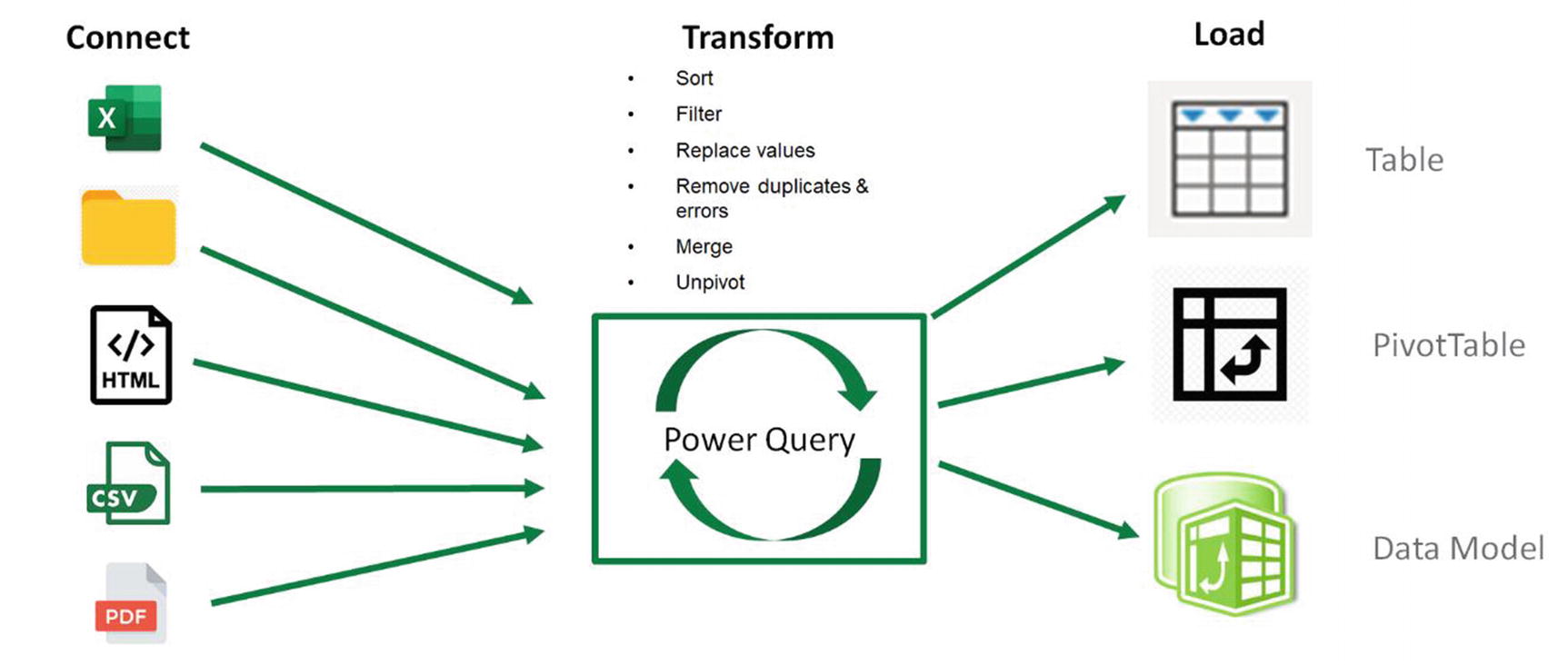
Connect, transform, and load data with Power Query
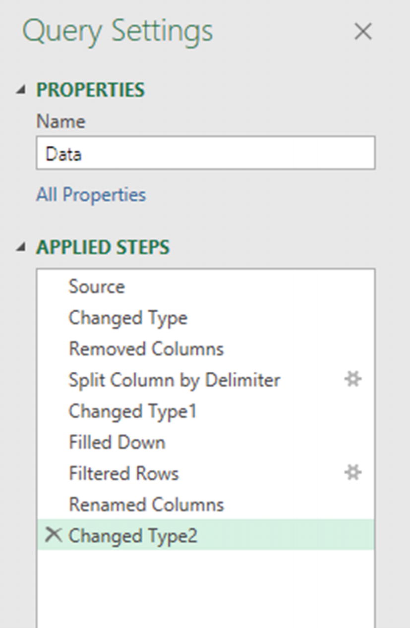
Each action in Power Query is recorded in Applied Steps
There is no Undo button in Power Query. You undo an action by deleting the applied step using the black X by the step name.
For each command, behind the scenes, M code was created. This is the language of Power Query. It can be complicated to learn, and fortunately you can do incredible things in Power Query without knowing any of it.

Methods to view and edit the Power Query M code
The examples in the chapter have been chosen to demonstrate as many features of Power Query as possible and barely any M code. There is far more to Power Query for you to explore beyond this chapter.
Transform Data in Excel
excel-data.xlsx
Let us look at our first example of using Power Query to clean and prepare data. This first example will be data already in Excel. However, this data has many problems and is not currently in a tabular structure for us to analyze with formulas, PivotTable, or other Excel features.

Unstructured data in Excel to transform
This is a typical example of data we can receive from software outputs or from other Excel users.
- 1.
Select the range B3:F30 and click Data ➤ From Table/Range.
- 2.
You will be prompted to format the range as a table. Check the My table has headers box.
- 3.
The table is loaded into the Power Query Editor. This is where all the magic happens. We should name the query first. Expand the Queries pane on the left, right-click the query, click Rename, and name it Data (Figure 5-6).
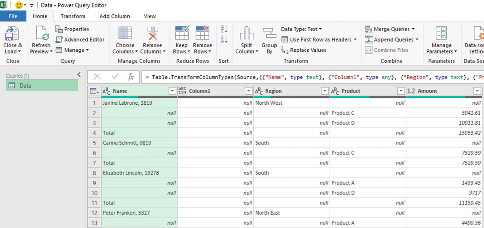
Data table loaded into the Power Query Editor
- 4.
Right-click the second column (named Column 1) and click Remove to delete this empty column.
- 5.
Select the Name column. Click Home ➤ Split Column ➤ By Delimiter. Select Custom from the list and enter a comma followed by a space (, ) as the delimiter (Figure 5-7).
This step splits the name and the ID into separate columns.

Split the column using the comma and space as the delimiter
- 6.
Select the Name.1, Name.2, and Region columns and click Transform ➤ Fill ➤ Down.
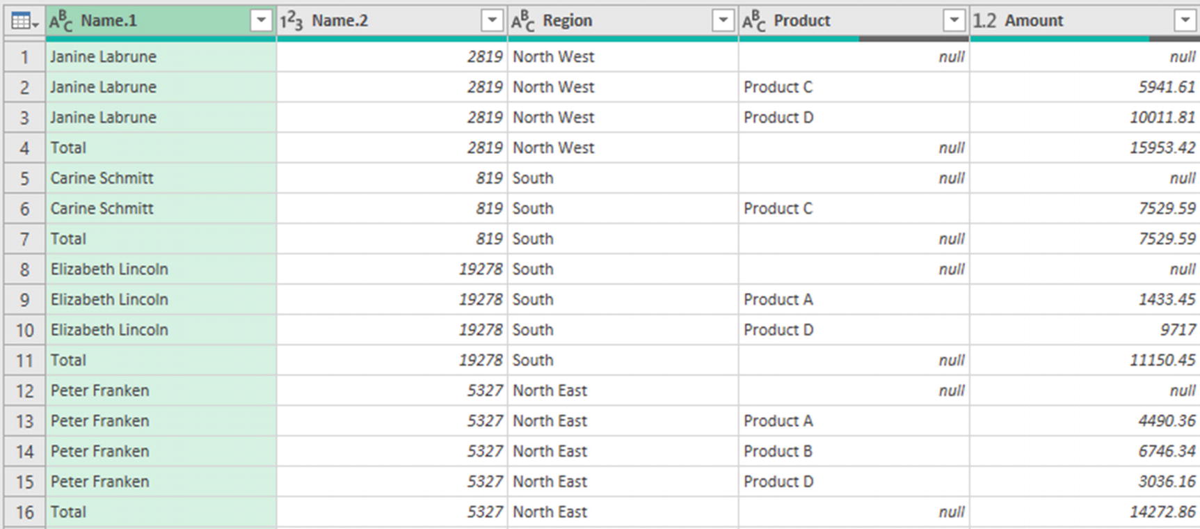
Data table with the empty cells from columns 1–3 populated
- 7.
Click the filter arrow in the Product column and uncheck the (null) box.
- 8.
Click and drag the Name.2 column to the first position so that the ID column is before the name column.
- 9.
Double-click the Name.2 header and rename it ID. Repeat for the Name.2 column and rename it Name.
- 10.
Click the data type button (Figure 5-9) in the Amount column header and change the data type to Currency.

Changing the data type to Currency for fixed decimal places
Do not confuse the data type with formatting. You will still need to format your cell and PivotTable values. Specifying the correct data type is critical to work with the data.

Applied Steps including multiple Changed Type steps
Multiple Changed Type steps have been produced by Power Query. Only Changed Type2 was directly actioned by us. This is not a problem, but we could delete Changed Type and Changed Type1 to tidy up the query and specify each column’s data type at the end ourselves, especially if the query was more elaborate than this one.

Warning as deleting a step may affect subsequent steps
You can stop Power Query from automatically adding Changed Type steps. Click File ➤ Options and settings ➤ Query Options and specify to never detect column types.
- 11.
Click Home ➤ Close & Load list ➤ Close & Load To. Specify Table to an Existing worksheet and select a cell to import to (Figure 5-12).
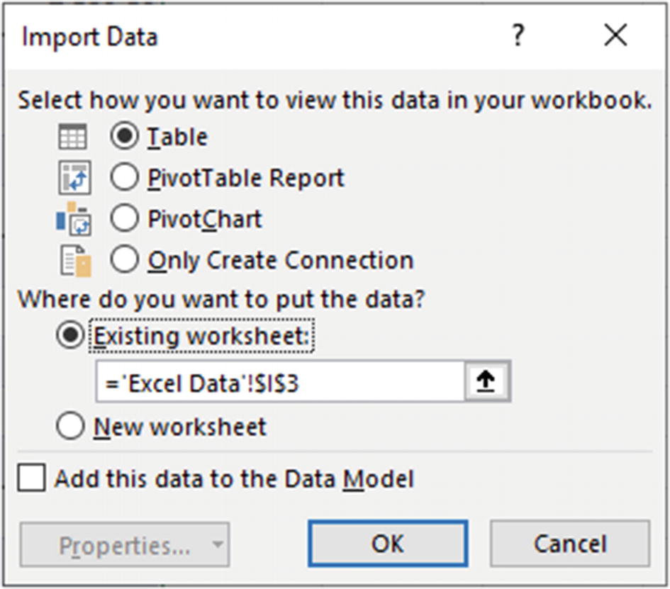
Close and load to a table on the existing worksheet
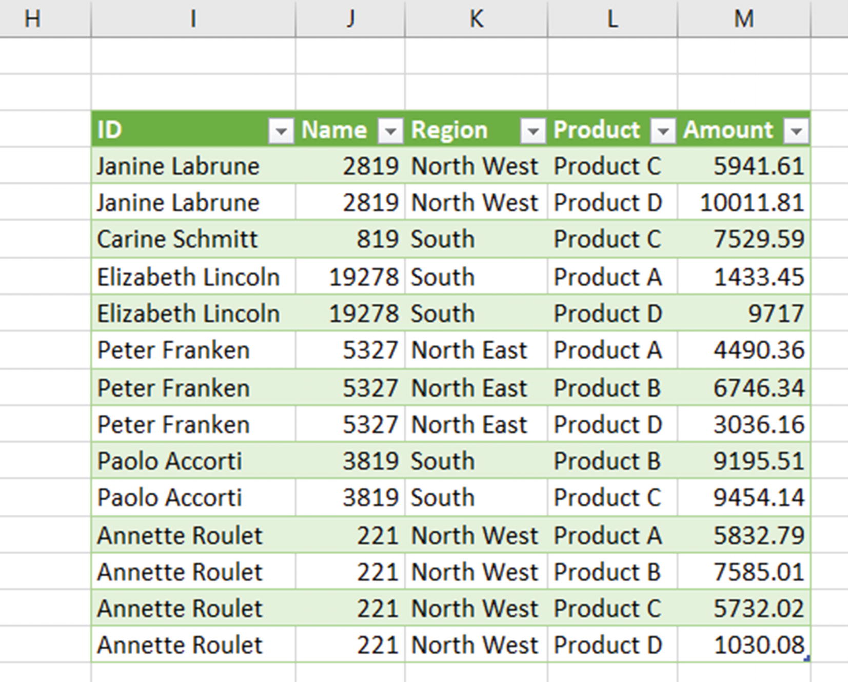
The transformed table is now easy to work with
If you need to edit the query, click the table and click the Query tab and then Edit, right-click the query in the Queries & Connections pane and Edit, or click Data ➤ Get Data ➤ Launch Power Query Editor to get access to all the workbook queries.
Combine Multiple Sheets into One
combine-tables.xlsx
A very common requirement in Excel is to combine multiple tables into one. The days of copying and pasting or using Macros are gone. Power Query makes this easy.
In this example, we have a workbook with 12 sheet tabs named after the months of the year (January–December). On each sheet, we have data formatted as a table (as it should be), and the tables are also named after the months of the year. The data is for product sales for that month, and each sheet has between 200 and 500 rows.
- 1.
Click Data ➤ Get Data ➤ From Other Sources ➤ Blank Query.
- 2.
The Power Query Editor opens, and you are taken to the Formula Bar (click View ➤ Formula Bar if you do not see one). Type the following formula:
The M language is case sensitive. So, check your typing and ensure it is exactly the same.
- 3.
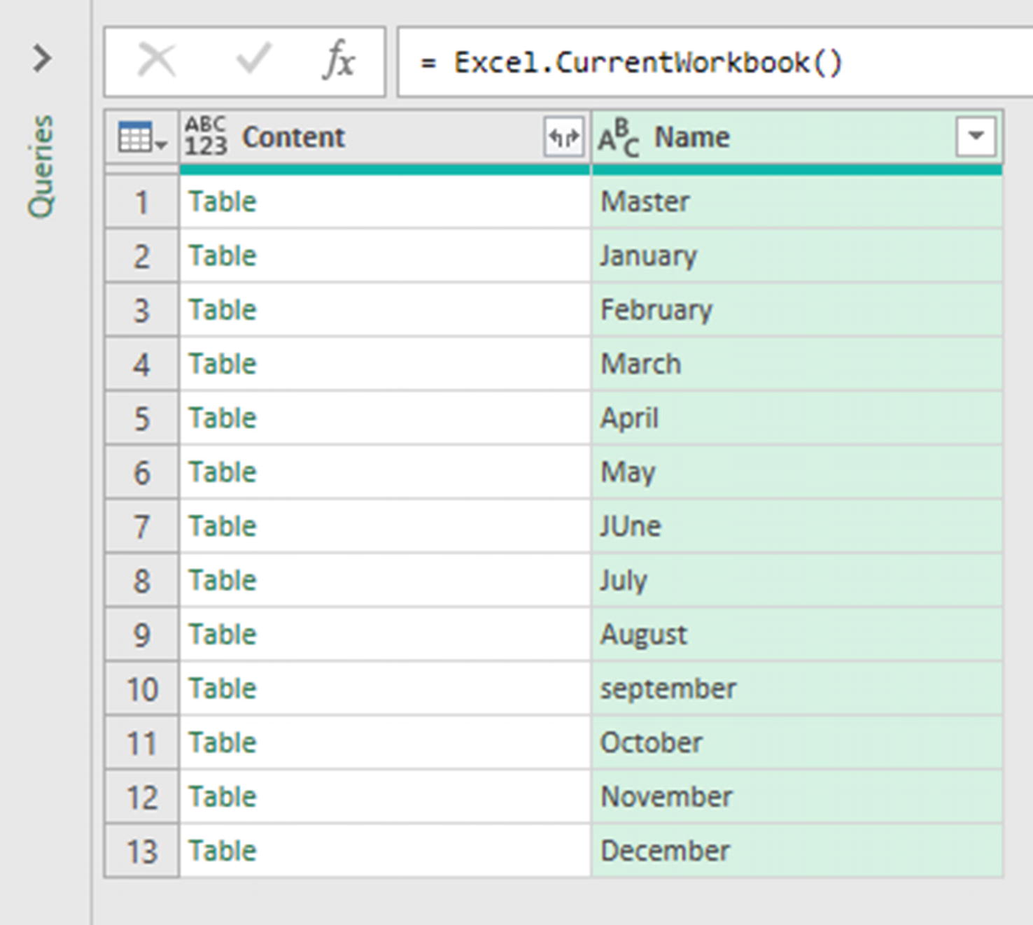
All the tables from the workbook are shown. We want to combine all of them into one table. Click the double arrow button in the Content column header (Figure 5-14).
Note If there were tables in the list we wanted to exclude, they could be filtered out at this stage.

Combine all the tables into one
- 4.
Ensure all the column boxes are checked to be included in the result. Uncheck the Use original column name as prefix box.
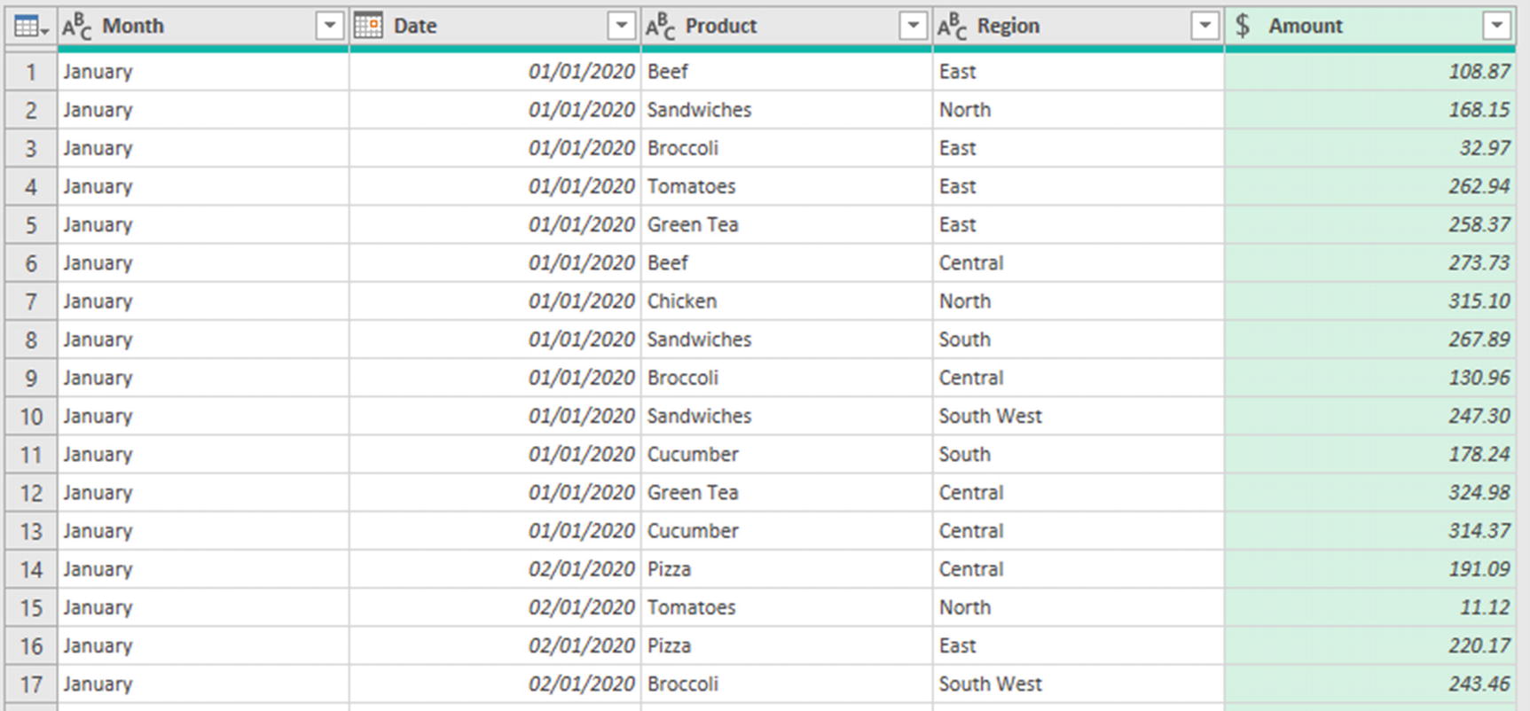
All the tables are expanded and stacked into one table. The table name is displayed in a column called Name. We do not really need this column as we have a Date column, but we will keep it as a label for our tables and charts.
- 5.
Rename the query Master.
- 6.
Move the Name column to the second position before the Product column.
We will shorten the month name to only the first three letters as this would work better in the axis of a chart.
- 7.
Select the Name column and click Transform ➤ Extract ➤ First Characters. Enter 3 as the number of characters.
There are also some irregularities in the format of these month names. In Figure 5-14, you can see that June has an uppercase U and September has a lowercase S.
- 8.
Click Transform ➤ Format ➤ Capitalize Each Word.
- 9.
Rename the Name column as Month.
- 10.
Change the data type of the Date column to Date, Product and Region columns to Text, and the Amount column to Currency.
- 11.
Click Home ➤ Close & Load list ➤ Close & Load To. Select Table and New worksheet.

Master query loaded 4434 rows
Excel.CurrentWorkbook() Problem
When data on any of those worksheets is changed, the query can be refreshed by clicking Data ➤ Refresh.
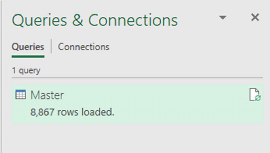
More rows loaded to the Master table on refreshing the query
This is happening because the Master query itself is a table in the workbook and is therefore included in the import.
- 1.
Right-click the Master query in the Queries & Connections pane and click Edit.
- 2.
Click the Source step in the Applied Steps box.
- 3.
Click Home ➤ Refresh Preview to see the Master table included in the list of tables (Figure 5-17).
Master table included in the list of tables to be appended
- 4.
Click the filter arrow for the Name column and uncheck the Master box.
- 5.
Click Home ➤ Close & Load.
Connect to Another Excel Workbook
another-excel-workbook.xlsx
Power Query also makes it simple to import data from an external Excel workbook. When changes are made to the Excel workbook, the connection can be refreshed to load the updates.
And if the workbook is renamed or has moved location, the query source can be edited easily without re-creating the entire query.
- 1.
From a blank Excel workbook, click Data ➤ Get Data ➤ From File ➤ From Workbook.
- 2.
Locate and select another-excel-workbook.xlsx.
- 3.
The Navigator window opens, listing all the tables, sheets, and defined names in the workbook (Figure 5-18). Check the Select multiple items box. Check the boxes for the Products table and the Angel, Bloomsbury, and Victoria sheets only.
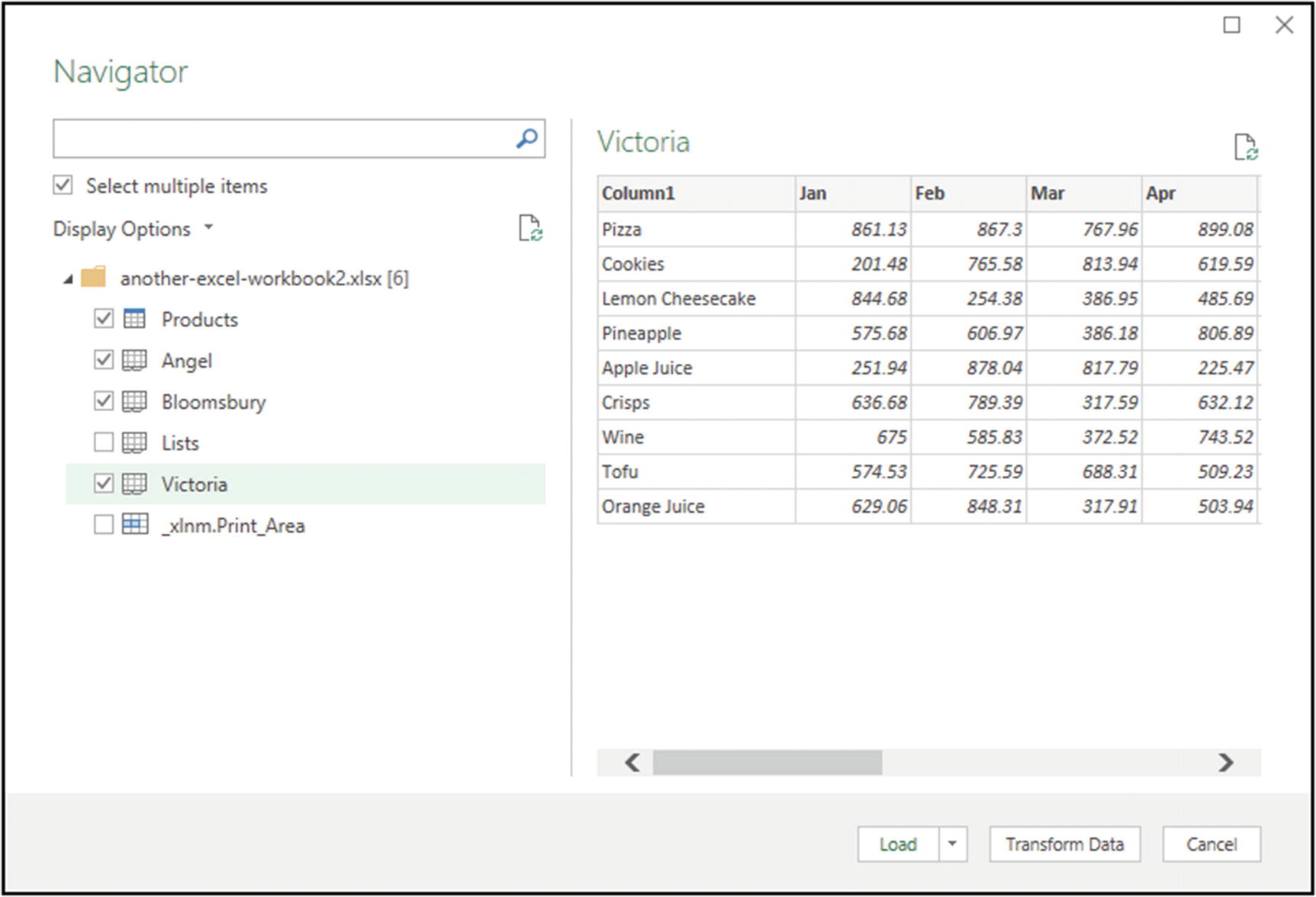
Select only the table and three of the worksheets to import
The defined name is for a print area that has been set, and the Lists sheet is the sheet where the Products table resides. We do not need these.
Instead of selecting the desired tables and sheets in this window, we could have filtered out those we do not want in the Power Query Editor. This approach is more dynamic as it will handle changes to the workbook such as additional print areas being created.
- 4.
Click Transform Data.
Each workbook item has been loaded as a separate query. The Products query is perfect. However, we need to perform some transformation steps on the other three.
We will append the Angel, Bloomsbury, and Victoria tables together to one table. But first we need to add a column with the name of the table to distinguish which store the sales came from when they are appended.
- 5.
Select the Angel query from the Queries pane on the left.
- 6.
Click Add Column ➤ Custom Column.
- 7.
Enter Store as the new column name and enter = "Angel" in the formula box provided (Figure 5-19).

Add a custom column with the table name
- 8.
Move the Store column to the first position in the table.
- 9.
We now need the month names and sales values in columns instead of rows. Select the Store and Column1 (product) columns. Right-click and click Unpivot Other Columns.
- 10.
Rename Column1 to Product, Attribute to Month, and Values to Amount.
- 11.
Change the data type of the Store column to Text and the Amount column to Currency.
The Angel query is now completed (Figure 5-20).
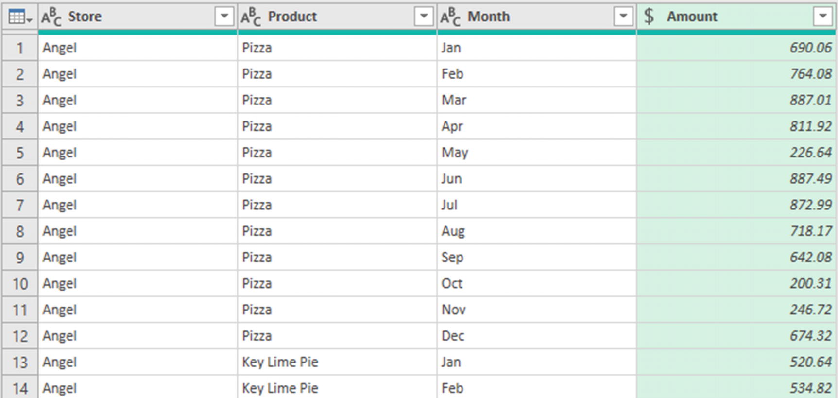
The completed Angel query
- 12.
Repeat steps 5–12 for the Bloomsbury and Victoria queries.
With the query for each store transformed, we will now append them into one sales table.
Note We could have appended the tables after adding the custom column and then only performed the unpivot, column naming, and data type steps once. I decided to keep the transformations local to the specific queries to make troubleshooting problems easier in the future.
- 13.
Select the Angel query and click Home ➤ Append Queries list ➤ Append Queries as New.
- 14.
Select the Three or more tables option, select the Bloomsbury table, and click Add and then repeat for the Victoria table (Figure 5-21).

Append query with three or more tables
- 15.
Name the query SalesCombined.
All three tables are stacked into one table. Perfect for a PivotTable or Excel functions such as SUMIFS to analyze.
The append query still references the three store queries. So, any changes to the Excel workbook, when refreshed, will update through to the SalesCombined query.
- 16.
Click Home ➤ Close & Load list ➤ Close & Load To. Select Only Create Connection.
All five queries are loaded, but they will not appear on the worksheet as they are connection only.
The three store queries were staging queries which we then appended. The Products query we will use in a Merge query shortly. The SalesCombined query is the only one we need to load to a table on the worksheet.
- 17.
Right-click the SalesCombined query in the Queries & Connections pane and click Load To.
- 18.
Select table and load it to the existing worksheet.
All five queries are loaded, but only the SalesCombined query is loaded as a table to the worksheet (Figure 5-22).
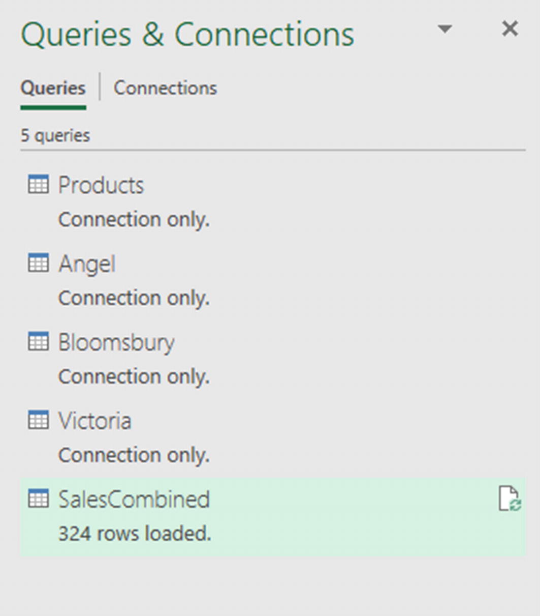
Five loaded queries, only one loaded as a table
- 19.
Save the workbook as store-sales.xlsx.
Merge Queries – A Lookup Alternative
store-sales.xlsx
Lookup formulas in Excel such as VLOOKUP, INDEX and MATCH, and XLOOKUP have many needs. They are incredibly versatile, and we saw demonstrations of some of their uses in Chapter 2. A popular use for them is to combine columns from different tables into one.
Merge Queries in Power Query are a fantastic alternative to this specific use of lookup formulas.
In this example, we will continue with the workbook from the previous section named store-sales.xlsx. We have a query named SalesCombined which contains data on product sales. And another query named Products which contains the category each product belongs to.
- 1.
Click Data ➤ Get Data ➤ Launch Power Query Editor.
- 2.
Select the SalesCombined query from the Queries pane.
- 3.
Click Home ➤ Merge Queries. This will merge to the currently selected query.
- 4.
Select Products from the list of tables to merge SalesCombined with.
- 5.
Click the Product column in the SalesCombined table and then the Product column in the Products table (Figure 5-23).
These are the two key fields to uniquely identify and link the products correctly. The message at the bottom of the Merge window confirms a complete match of 324 out of 324 rows.
Note You can select multiple columns to identify records correctly from two tables. For example, it could be product name and size.
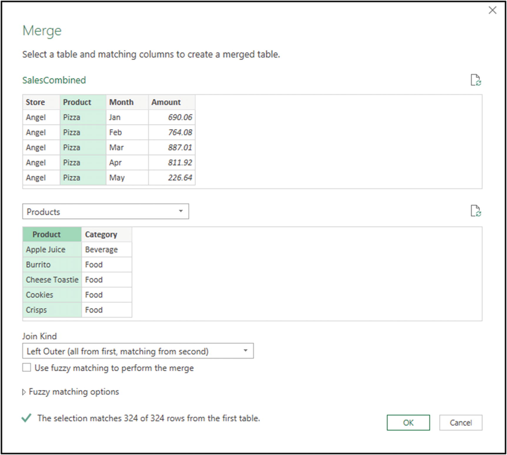
Merge query to add columns from another table
- 6.
The Join Kind is set to Left Outer. This is what we need for this example. There are six different join kinds.
- 7.
The Products table is added as a column to the SalesCombined query. Click the double arrow button in the column header. Uncheck the Product column and the Use original column name as prefix box (Figure 5-24).

Add the Category column to the SalesCombined table
- 8.
Move the column to the third position after the Product column.
- 9.
Click Home ➤ Close & Load.
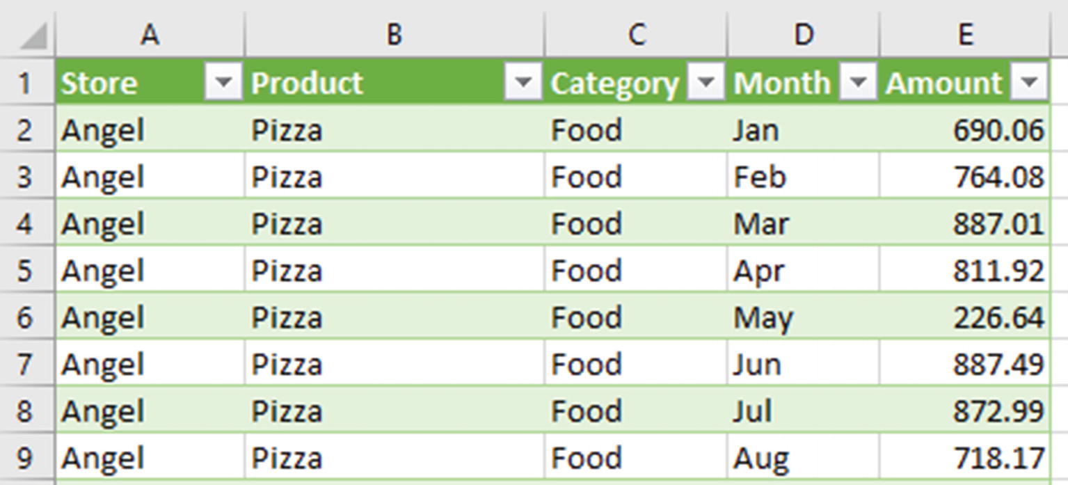
Completed SalesCombined table with added category column
Merge Queries – Compare Tables
merge-queries-compare.xlsx
There are five other join kinds in addition to the classic merge we have just seen. The different join kinds will return different results, so the one you choose will depend on the result you want.
Left Outer: All rows from the left table and only the matches from the right (classic lookup)
Right Outer: All the rows from the right table and only the matches from the left
Full Outer: All rows from both tables
Inner: Only the matching rows from both tables
Left Anti: Rows in the left table without a match in the right table
Right Anti: Rows in the right table without a match in the left table

Two tables with event attendees to compare
The tables contain the names of attendees for two events. We would like to compare the two tables to output the names of those who attended both events. And another query with the names of those who attended event 2, but not event 1. These attendees are new visitors.
- 1.
Click Data ➤ Get Data ➤ Combine Queries ➤ Merge.
- 2.
Select Event1 from the first list of tables and Event2 from the second list.
- 3.
Click the Name column in Event1 and then again in Event2. This is the identifying value in both columns.
- 4.
Select Inner from the Join Kind list (Figure 5-27).
This will produce the results of those who attended both events. The preview text at the bottom of the window informs us that there will be eight names returned.

Perform an inner join between two tables
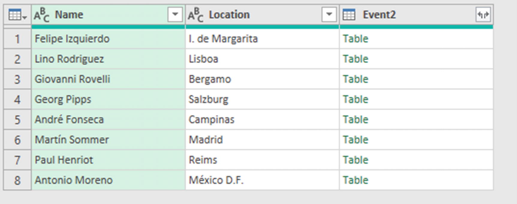
Eight rows appear in both the left and the right tables
The right table is added as a column. We used this in the previous example to add columns to the left table. This time, it is unnecessary as the left and right tables have the same columns.
- 5.
Name the query AttendedBoth.
- 6.
Close and load the query as a table to the worksheet.
- 1.
Start another merge query with the two tables and specify the Right Anti from the Join Kind list.
- 2.
Name the query Event2Only.
Figure 5-29 shows the results of the right anti join. This join returns rows that exist in the right table only. Therefore, the left table returns no rows, and we need to expand the right table to get the results.
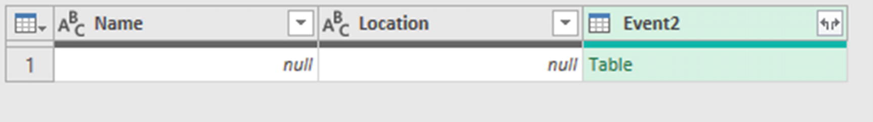
Right Anti join results
- 3.
Click the double arrow button in the Event2 header, keep both columns checked, and uncheck the Use original column name as prefix box.
- 4.
Remove the first two columns and rename the Name.1 column to Name and the Location.1 column to Location.
- 5.
Close and load the query as a table to the worksheet.

The results from both merge queries
The six different joins of merge queries can be very useful. Explore their capabilities and think about scenarios where they could prove useful to you.
Import Files from a Folder
sales-data folder
This feature of Power Query is magnificent. The hours of time I have saved many users by demonstrating this functionality are “off the chart.”
With Power Query, it is simple to import all or just some of the files from a folder. You choose which files to import by specifying filter criteria on the file attributes such as name, extension, or date modified. Or import them all and filter out the content you do not need.
This connection can then update with the click of a button when files are added, removed, or changed in that folder.

The sales-data folder with the CSV files to import
It also contains a text document named exciting and a PDF file named new-members. We have no interest in using these files in this query.
For this query, we will load it directly into a PivotTable. Most of the previous queries have been loaded as a table to the worksheet. This is great as you can continue using Excel tools with the data.
However, if the goal is to analyze the data with a PivotTable or load it into the data model (covered in Chapter 6) for further analysis, then it is unnecessary to store it on the worksheet. And doing so will add unnecessary bulk and weight to your Excel file.
- 1.
Start a new workbook and click Data ➤ Get Data ➤ From File ➤ From Folder.
- 2.
Click Browse and locate the sales-data folder (Figure 5-32).
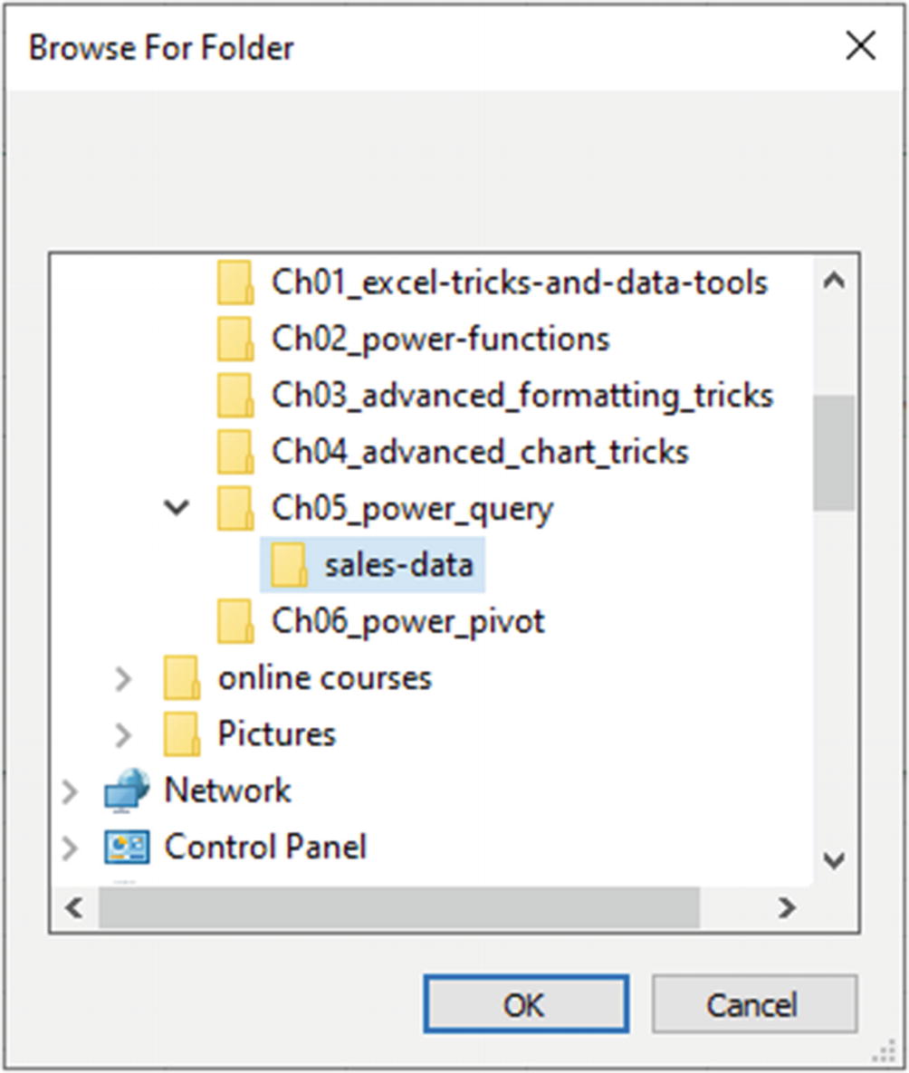
Locate the sales-data folder
- 3.
A window appears listing all the files found in that folder. Click Transform Data.
There are buttons in this window to combine or load the files. It is good practice to click Transform Data, even if your intent is to combine or load the files. This gives you the chance to check the quality of your data and make any required transformations.
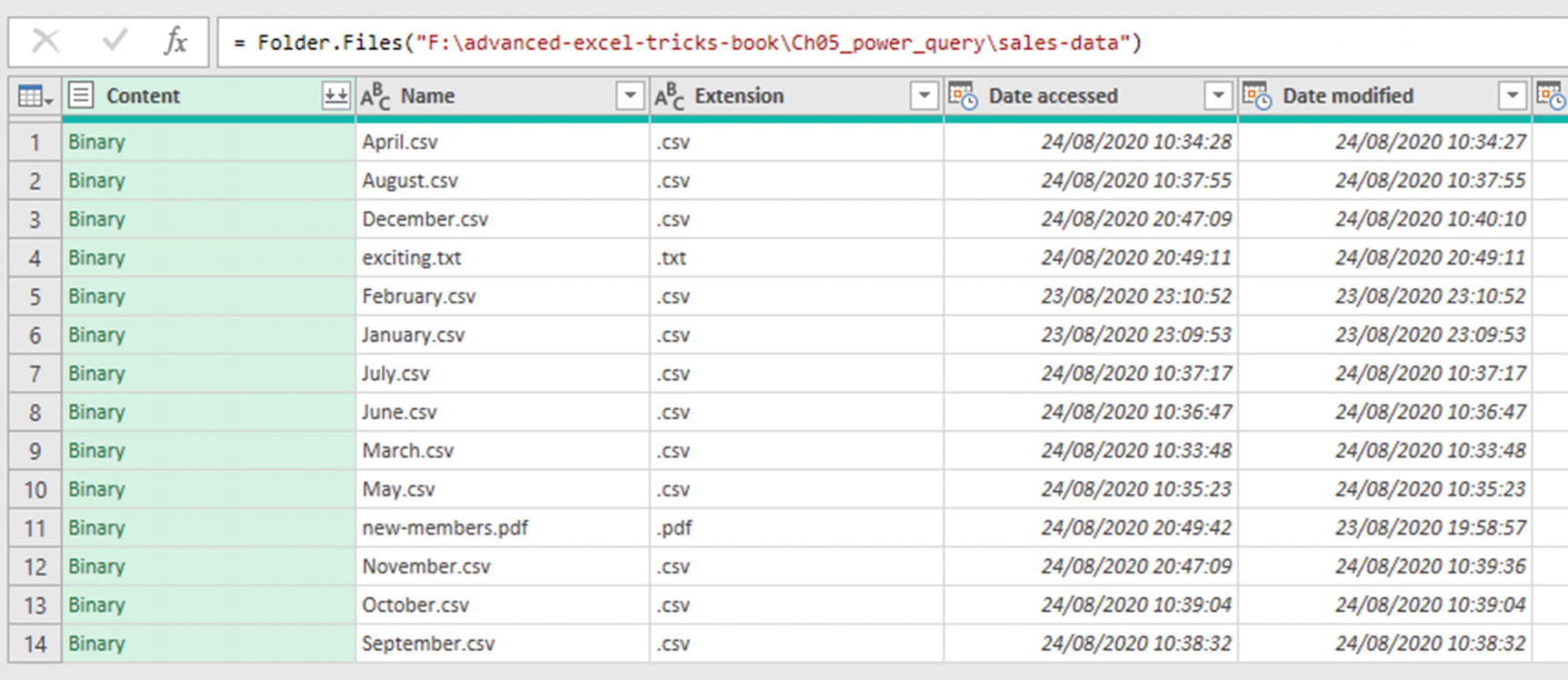
All content from the folder is loaded into Power Query
- 4.
Click the filter arrow for the Extension column and clear the check boxes for the .pdf and .txt extensions.
Even though our action was to remove the pdf and txt files, the step created was to include CSV files only. This is what we wanted. So, it is important that it did not record our specific actions.
To explain further, if it had recorded the specific actions of removing pdf and txt files, there would be problems if an avi, png, or pptx file was to appear in that folder in the future.
You could also have filtered the list using the Text Filters option in the filter list. These options are great for more flexible filter criteria. For example, to filter for extensions that begin with .xls would also include .xlsx, .xls, .xlsm, and .xlsb files.
- 5.
Click the Combine Files button (double arrow in the Content header).
- 6.
In the Combine Files window, you can specify a sample file from the list. This is the file that Power Query will follow as a framework for the other files when appending them. These files all have the same column headers, so the first file (April.csv) is fine for this example.
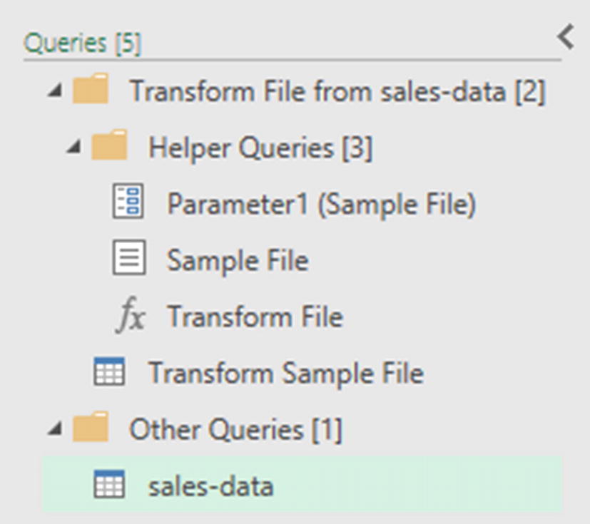
Multiple queries in the Queries pane
- 7.
With the Source.Name column selected, click Home ➤ Replace Values. Enter .csv as the Value To Find and leave the Replace With box empty (Figure 5-35).
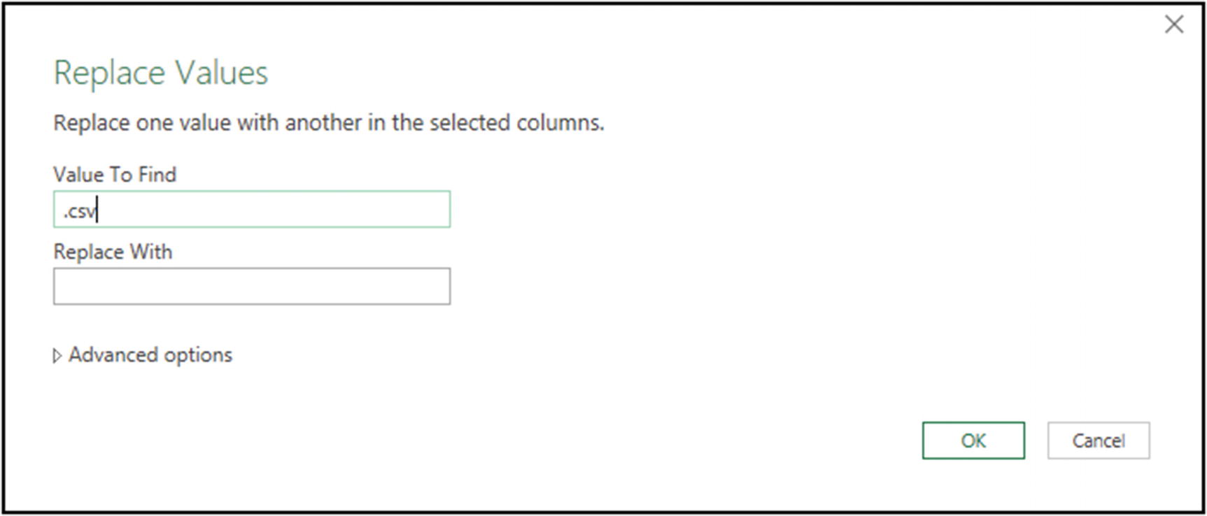
Using Replace Values to remove the CSV file extension
- 8.
Rename the Source.Name column as Month.
- 9.
Select the Date column and click Home ➤ Sort Ascending.
- 10.
Change the data type of the Amount column to Currency.
- 11.
Rename the query as AllMonthsSales.
Imported and transformed CSV files from the sales-data folder
- 12.
Click Home ➤ Close & Load list ➤ Close & Load To.
- 13.
Select PivotTable Report and place it on an existing worksheet.
PivotTable showing product sales in descending order by sales total
The data exists nowhere physically on a worksheet. Power Query connects the folder to the PivotTable. On clicking Data ➤ Refresh ➤ Refresh All, it would pull in all the CSV files, perform the transformation steps, and update the PivotTable.
Extract Data from the Web
The Web is full of information that we may be interested in pulling into our Excel spreadsheets. Unfortunately, this is not always as simple as we would wish due to how the web page has been structured. And this is often out of our control.
Power Query provides a friendly interface to import data from the Web, but it does rely on the required data being formatted as a table on the web page.
There are continuous improvements in Excel’s ability to extract data from the Web. Hopefully, since the publication of this book, there will be extra features to help extract less structured data from the Web.

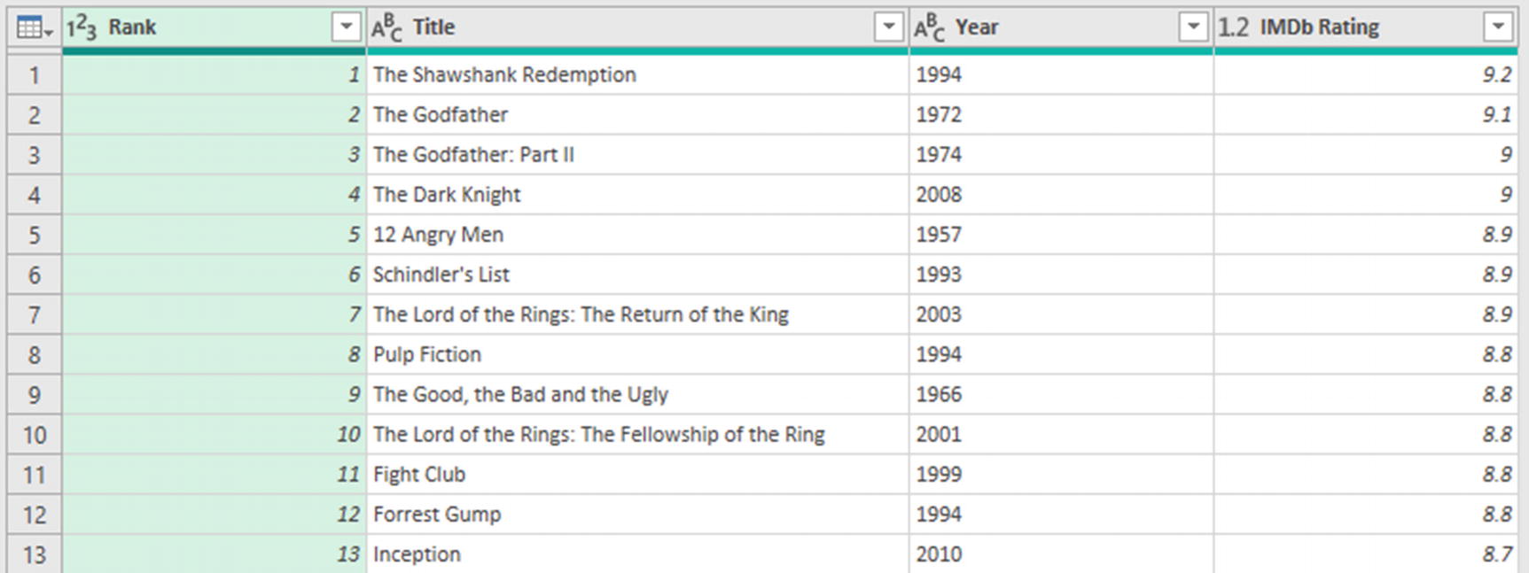
The IMDb top 250 films to be imported
On importing the data, we will extract the year that the films were released into its own column and create a custom column with the decade of each film’s release.
- 1.
Click Data ➤ Get Data ➤ From Other Sources ➤ From Web.
- 2.
Enter the following URL into the box provided (Figure 5-39):

Enter the URL of the page to import into Excel
This URL may have changed since the publication of this book. Enter “IMDb top 250” into a search engine to grab the most up-to-date URL.
- 3.
In this example, only the document itself and one table are returned. Select Table 0 and click Transform Data.
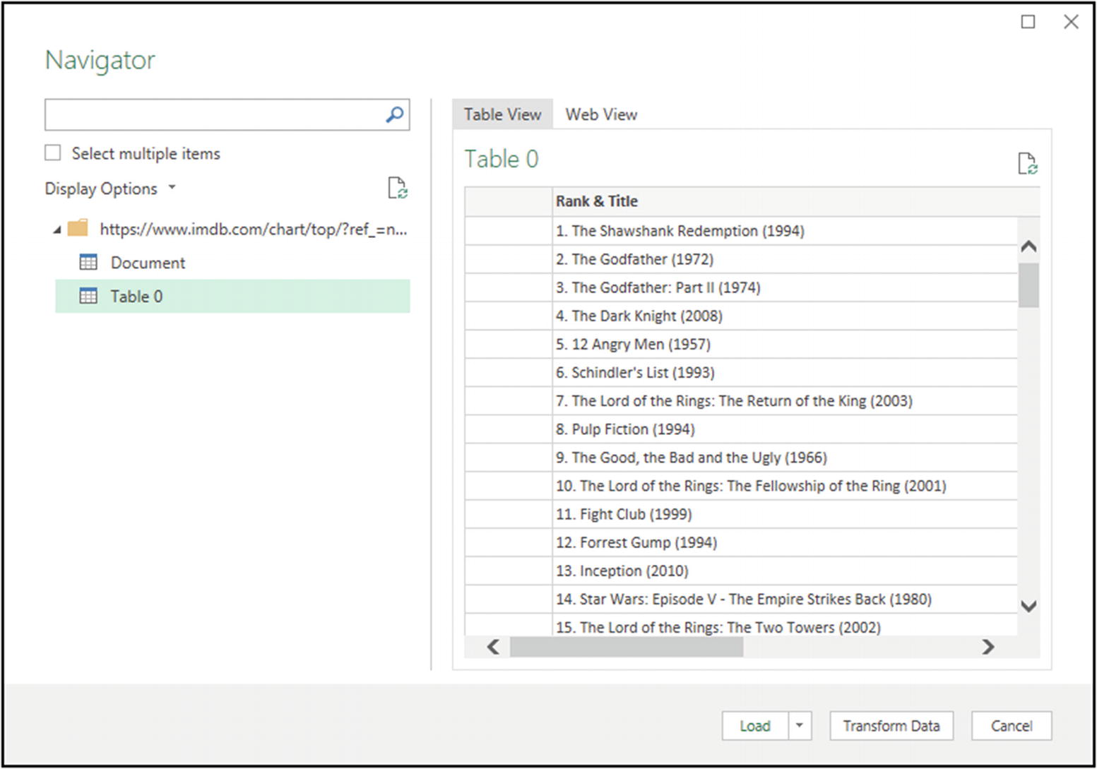
Select the table from the web page to import
- 4.
In the Power Query Editor, rename the query TopFilms.
Figure 5-41 shows the data loaded into Power Query. There are a few transformations to walk through to get the rank, title, year, decade, and rating columns that we want.
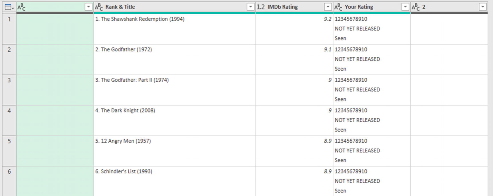
Top 250 film data loaded into Power Query
- 5.
Select the Rank & Title and IMDb Rating columns and click Home ➤ Remove Columns list ➤ Remove Other Columns.
Let us split the rank and title into separate columns.
- 6.
With the Rank & Title column selected, click Home ➤ Split Column ➤ By Delimiter. Use a custom delimiter and enter a full stop (period) followed by a space (. ) (Figure 5-42). Select Left-most delimiter as some of the film titles include full stops in their name.
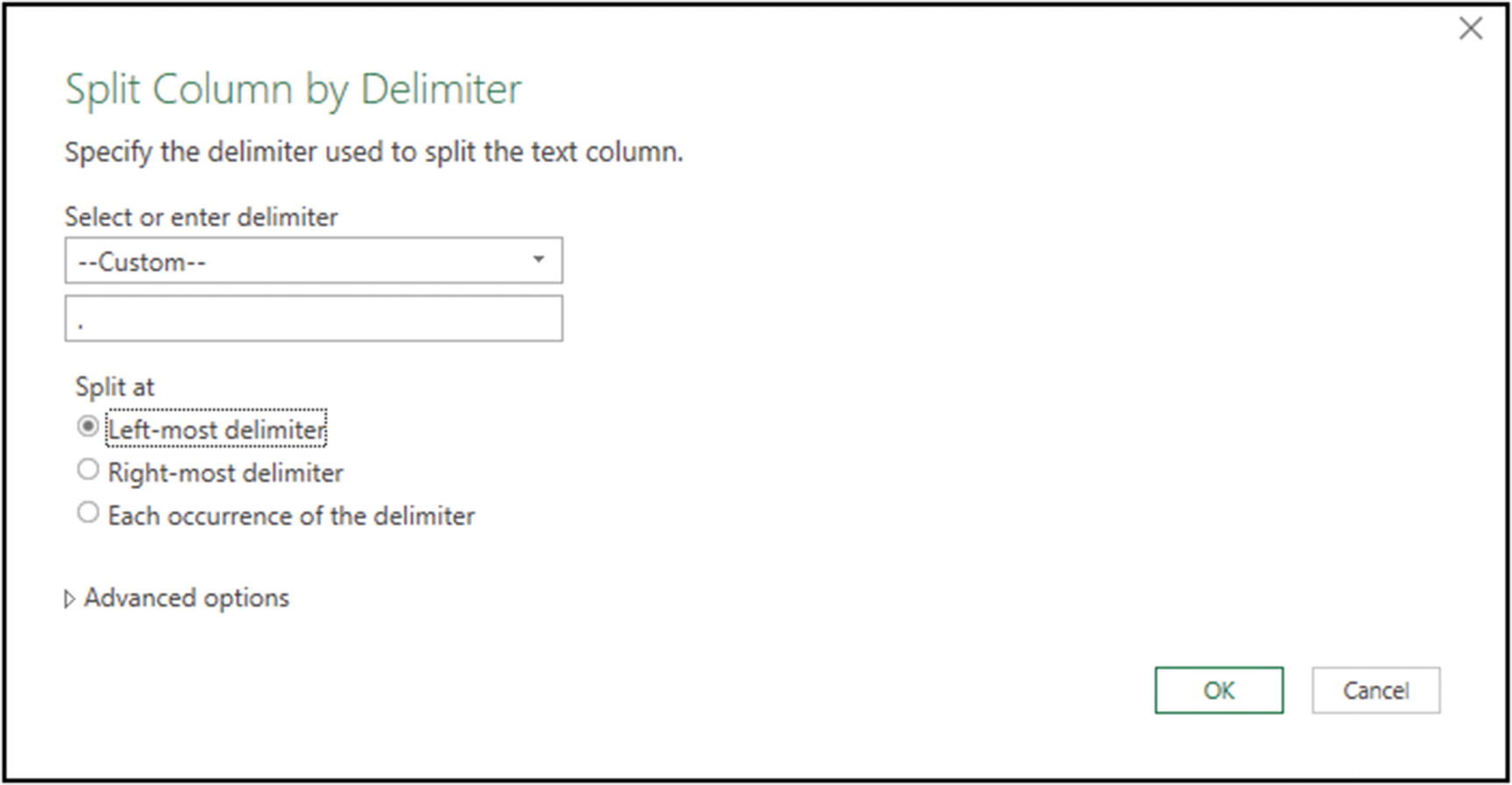
Splitting the rank and film title into separate columns
- 7.
Select the Rank & Title.2 column and click Home ➤ Split Column ➤ By Delimiter. Use a custom delimiter and enter a space followed by an opening parenthesis “ (”.
- 8.
To remove the closing parenthesis from the year, select the Rank & Title.2.2 column and click Home ➤ Replace Values. Enter a closing parenthesis “)” for the Value To Find and leave the Replace With box empty.
- 9.
Rename the first column to Rank, the second column to Title, and the third column to Year.
Figure 5-43 shows the progress so far with the TopFilms query.
Transforming the IMDb top 250 films table
- 10.
Select the Year column and click Add Column ➤ Column From Examples list ➤ From Selection.
We will now enter example values for the rows, and Power Query will try and work out what we need.
- 11.
Enter 1990-1999 for the first film into the column provided on the right and press Enter. This film (your list may be different as it changes over time) was released in 1994 so 1990–1999 is the decade.
Column From Examples’ first attempt to understand what we need is incorrect (Figure 5-44).
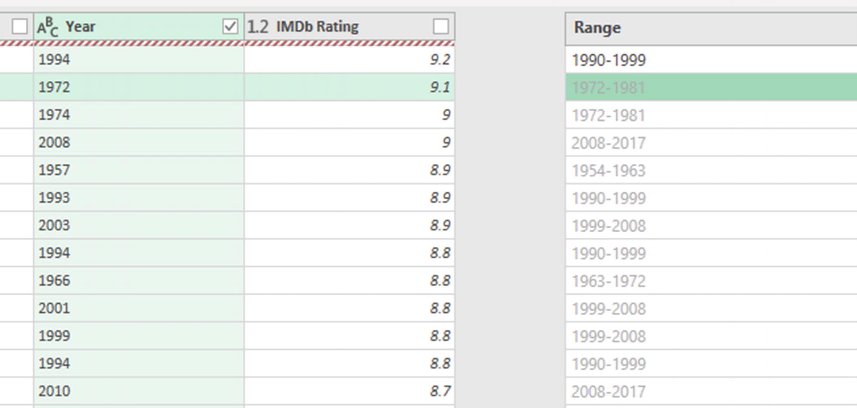
First attempt by Column From Examples
- 12.
Enter 1970-1979 for the second film and press Enter. Column From Examples has now successfully understood what we want (Figure 5-45). Click OK.
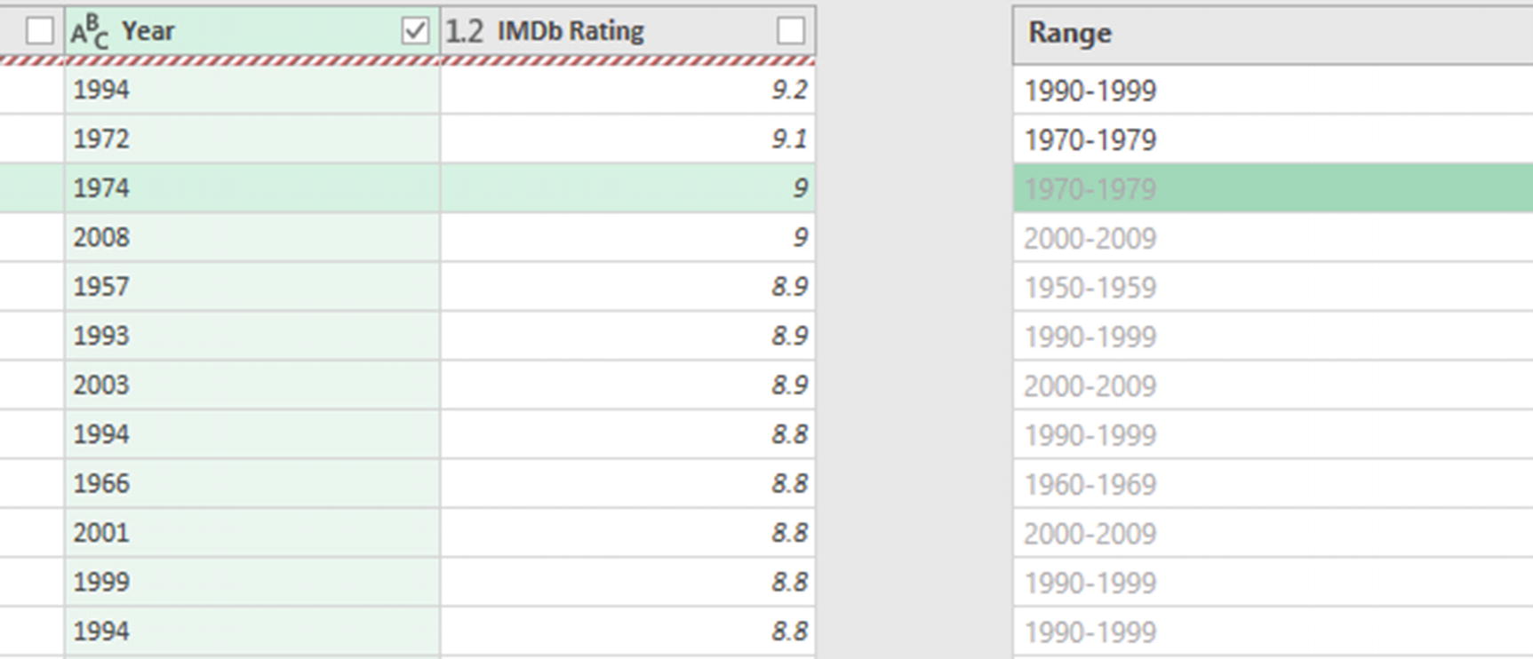
Column From Examples to create a custom column
- 13.
Click and drag the Range column to between the Year and IMDb Rating columns.
- 14.
Rename the Range column to Decade.
- 15.
Change the data type of the Year column to Whole Number.
All the transformation steps of the query are complete. However, we could clean up the Applied Steps box.
Earlier in this chapter, we covered deleting the Changed Type steps. We can also rename steps. For example, we have two split column steps. Renaming these will provide more transparency to the query steps.
- 16.
Right-click the Split Column by Delimiter step and click Rename. Name this step Split Rank and Title.
- 17.
Right-click the Split Column by Delimiter1 step and click Rename. Name this step Split Title and Year.
You will be thankful for the time taken to rename steps when you revisit the query in the future. It will be much easier to understand. Figure 5-46 shows the Applied Steps after renaming the two split column steps.
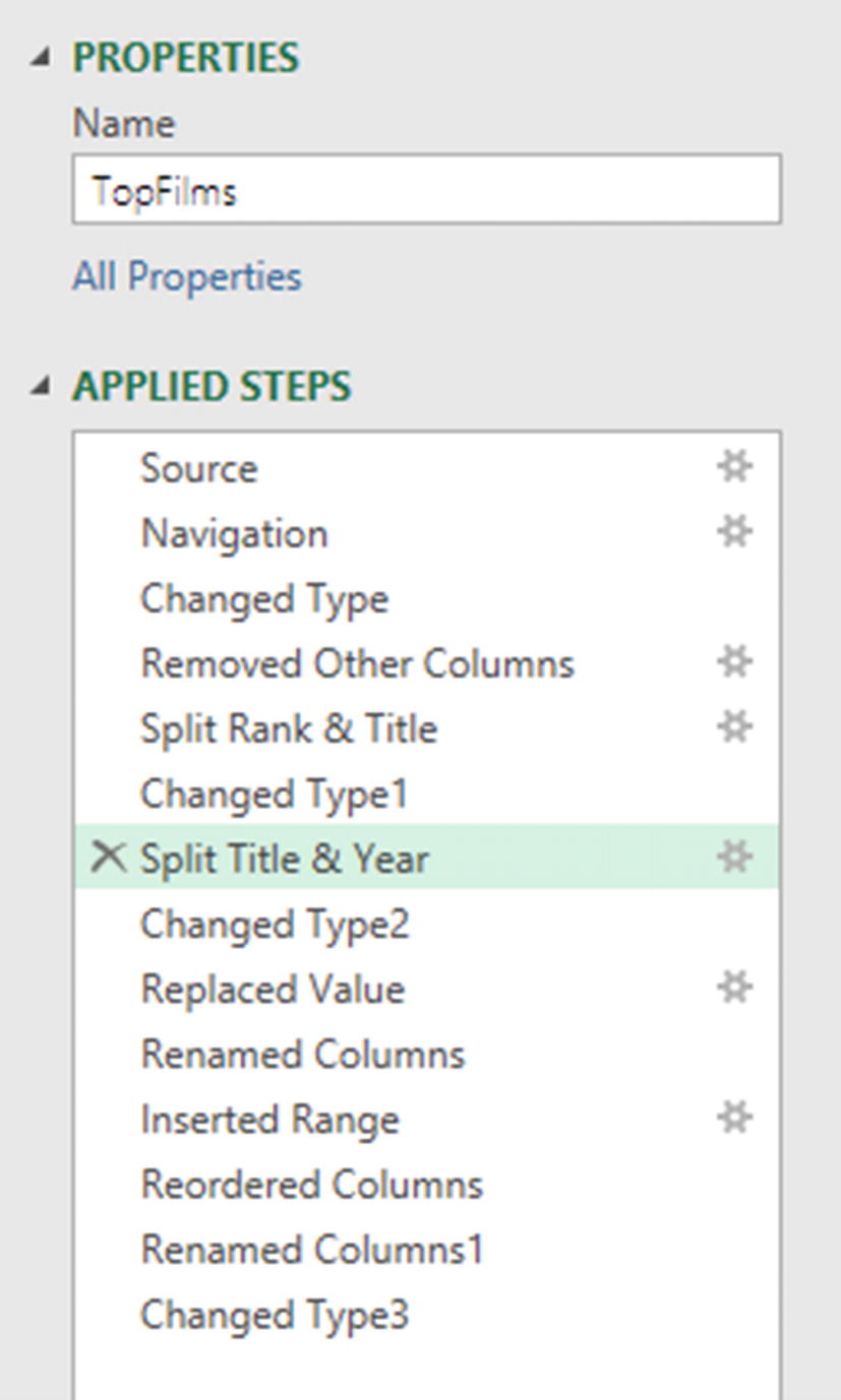
Applied Steps with steps renamed for greater meaning
The gear icon to the right of the steps can be used to edit the step. If a step does not have a gear icon, it can only be edited with the M code in the Formula Bar or Advanced Editor.
- 18.
Close and load the query as a table to a worksheet.

PivotTable showing the count of films by decade
Import from PDF
new-members.pdf
Power Query also makes it easy to import PDF data into Excel. We can then clean and tidy the data as we need it.
- 1.
Click Data ➤ Get Data ➤ From File ➤ From PDF.
- 2.
Locate the new-members.pdf document and click Import.
In the Navigator window, Power Query lists all of the tables and pages that it has identified in the document (Figure 5-48). The table with new member data that continues over three pages has been identified as three different tables by Power Query (tables 2, 3, and 4).
The preview area in the window is great to help discern the different tables.
- 3.
Check the Select multiple items box and check the boxes for Table002, Table003, and Table004.
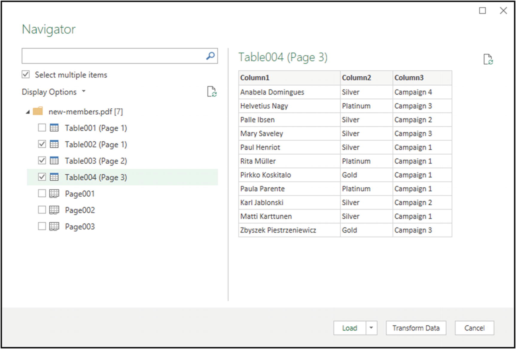
Select the tables to import from the PDF
- 4.
Click Transform Data.
The three tables are imported as separate queries (Figure 5-49). These queries make up the three parts of the new members data table, so we will append them shortly.
Firstly, let us tidy up the table headers. In the first query, the first row of data are the headers.
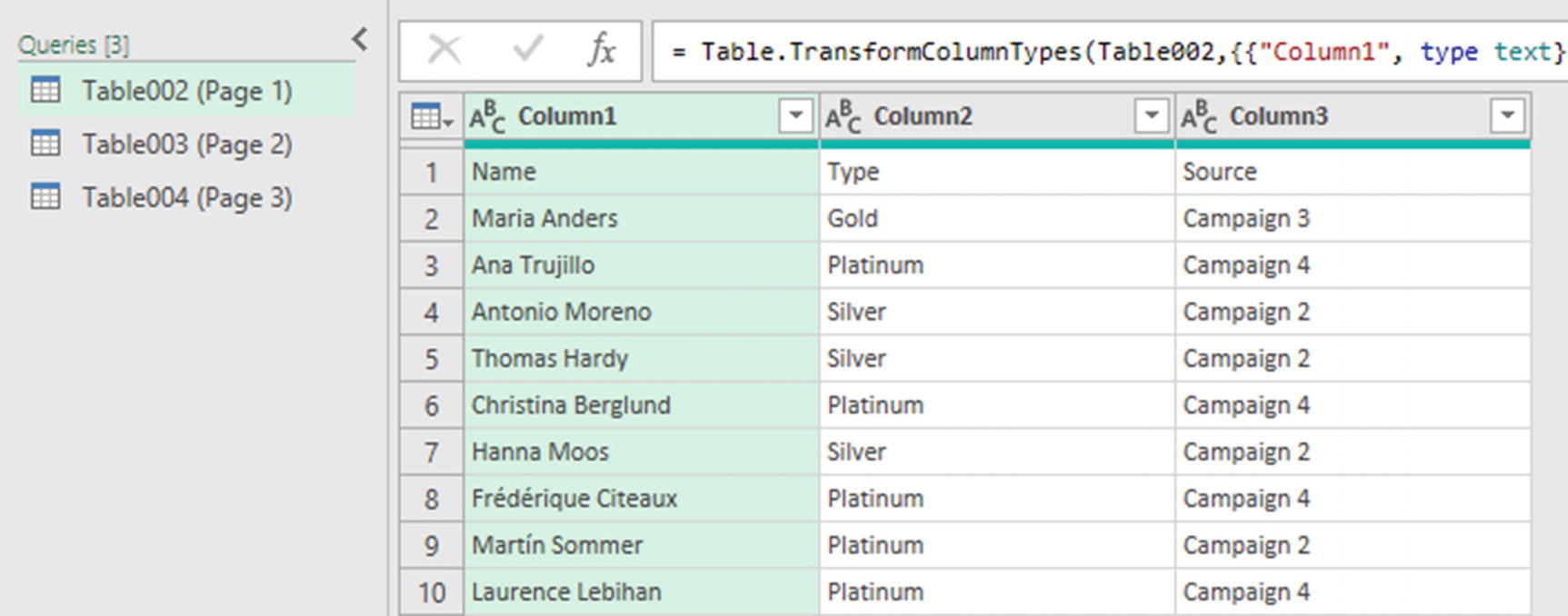
Tables are imported from the PDF as separate queries
- 5.
Ensure that the Table002 (Page 1) query is selected and click Home ➤ Use first row as headers.
- 6.
Select Table003 (Page 2) and rename the headers Name, Type, and Source to match the headers used in Table002. Repeat for Table003 (Page 3).
- 7.
Select Table002 (Page 1) and click Home ➤ Append Queries list ➤ Append Queries as New.
- 8.
In the Append window, select Three or more tables. Add the two other tables to the Tables to append box (Figure 5-50).
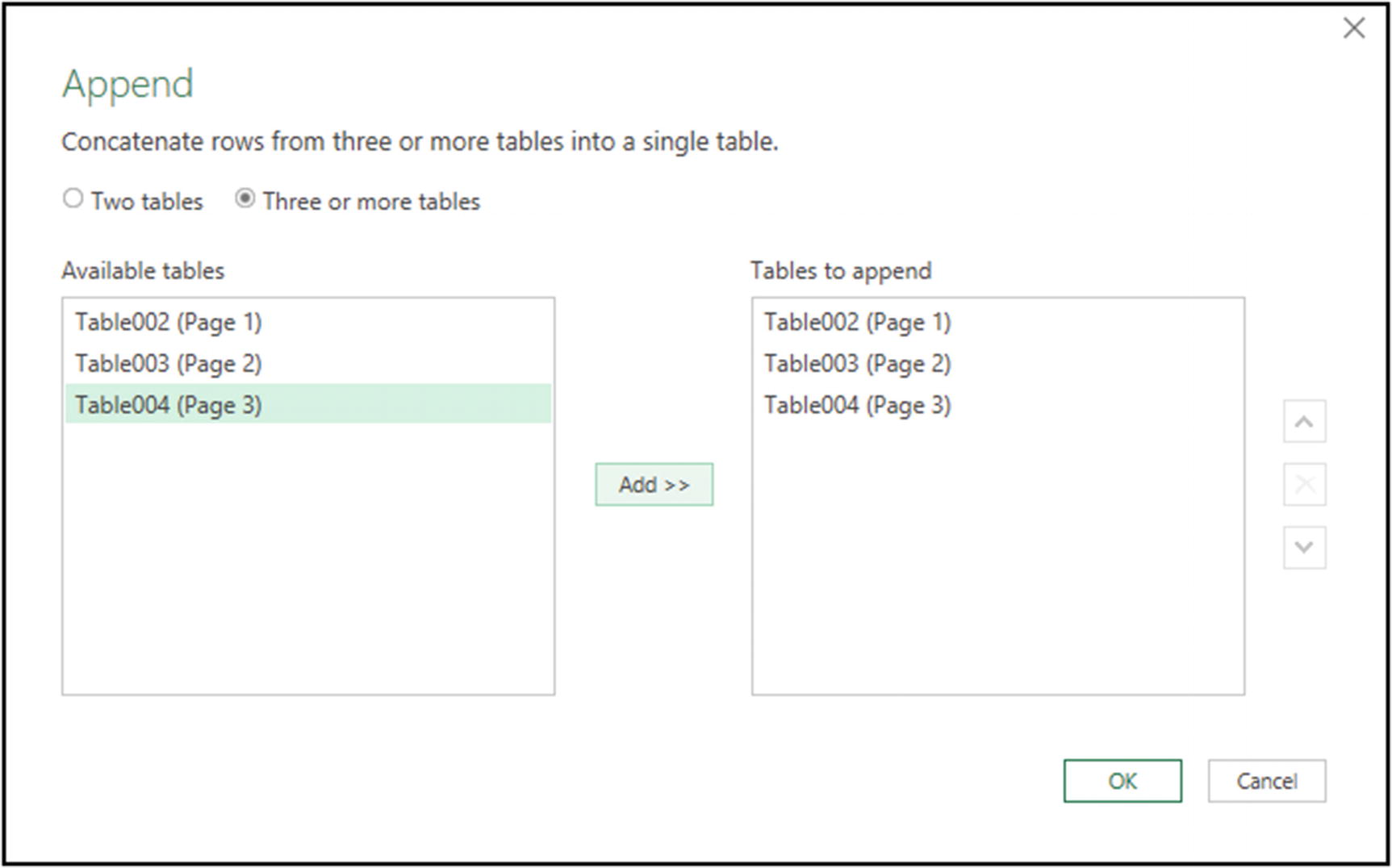
Append all three tables imported from the PDF
- 9.
Name the query NewMembers.
- 10.
Close and load it as a table to the worksheet.
Group By and Pivot
group-by-and-pivot.xlsx
Power Query is typically used to import and prepare data for a PivotTable or Excel formulas to summarize. However, Power Query itself has the functionality to group, summarize, and pivot data.
- 1.
Right-click the Master query in the Queries & Connections pane (click Data ➤ Queries & Connections if it is hidden) and click Load To.
- 2.
Select Only Create Connection and click OK.
- 3.
Changing the query back to a connection only query will remove the table on the worksheet (Figure 5-51). Click OK to confirm this.

Warning as the connection only query will remove the table
The first report will show the total sales from the regions for all months of the year (Figure 5-52).

Monthly sales by region report
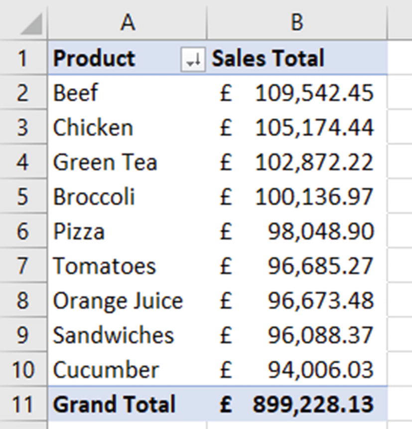
The second report will show the total sales and number of sales for each product. This will be sorted in descending order by total sales (Figure 5-53).

Total and number of sales by product report
- 1.
Click Data ➤ Get Data ➤ Launch Power Query Editor.
- 2.
Right-click the Master query and click Reference. Repeat this step so that we have two new queries.
- 3.
Rename one of the queries MonthlySalesByRegion and the other query ProductSales.
This creates two queries that are linked to the Master query. This ensures that the combining of the sheets and the transformation steps is only performed once, and then the two query reports are run. It’s better than duplicating a query and unnecessarily repeating the steps.

Viewing the dependencies between the queries
- 4.
Select the MonthlySalesByRegion query and click Home ➤ Group By.
- 5.
Select Advanced so that we can group by more than one column. Select Region from the list, click Add grouping, and then select Month from the second list (Figure 5-55).
- 6.
Enter Total for the new column name and specify the operation as Sum and the column to sum as Amount.
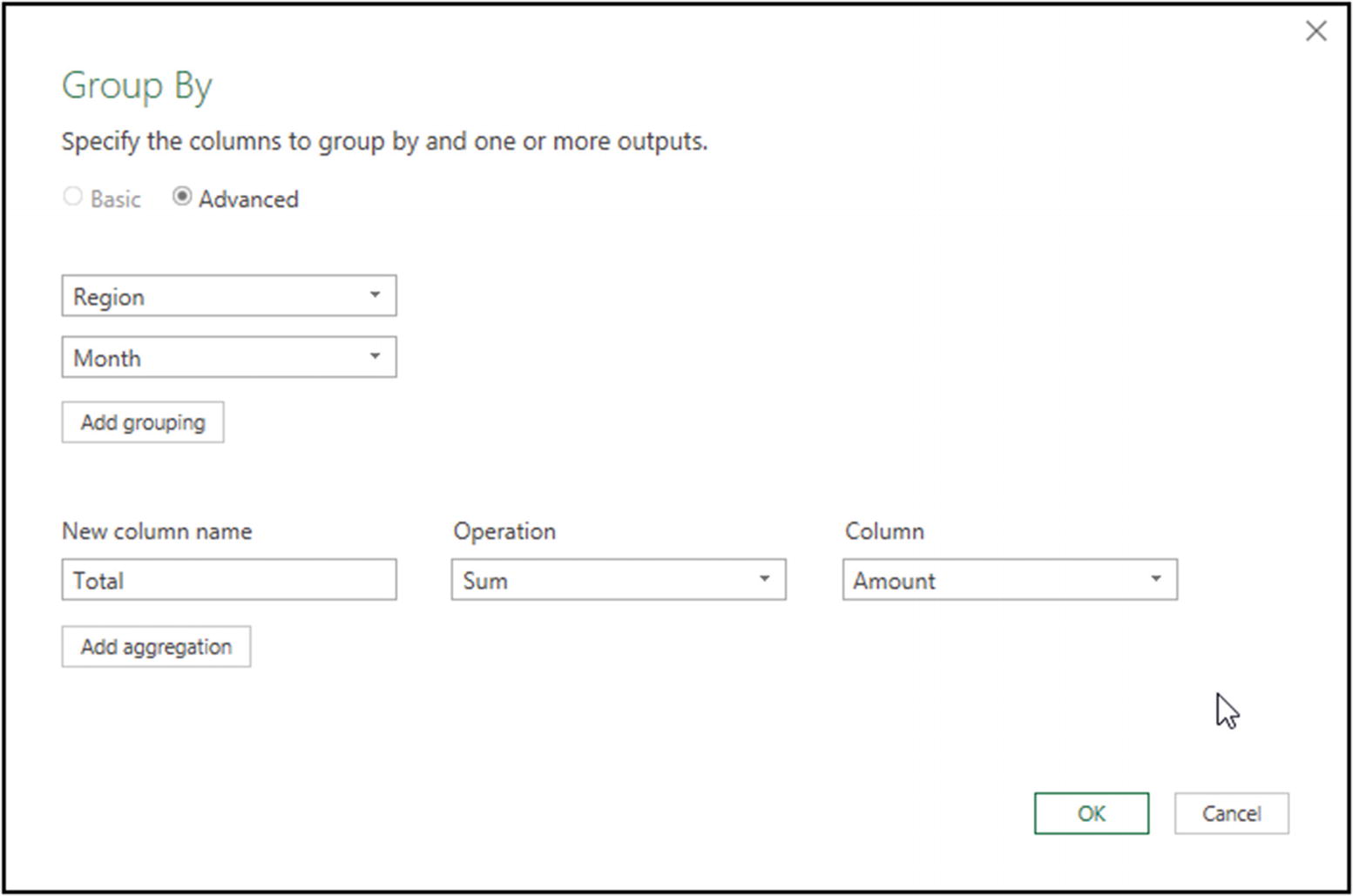
Group by region and month with total sales

Group by region and month
- 7.
Select the Month column and click Transform ➤ Pivot Column.
- 8.Select Total as the Values Column and click OK (Figure 5-57).
 Figure 5-57
Pivot the month column to become column headers
- 9.
Select the Jan column, press Shift, and select the Dec column. Click Home ➤ Data Type list ➤ Currency.
Let us now create the second report.
- 10.
Select the ProductSales query and click Home ➤ Group By.
- 11.
Select Advanced and select the Product column to group by.
- 12.
This report has two aggregations. For the first one, enter Total Sales for the column name and to Sum the Amount column. For the second aggregation, use No of Sales for the column name and Count Rows for the operation (Figure 5-58).
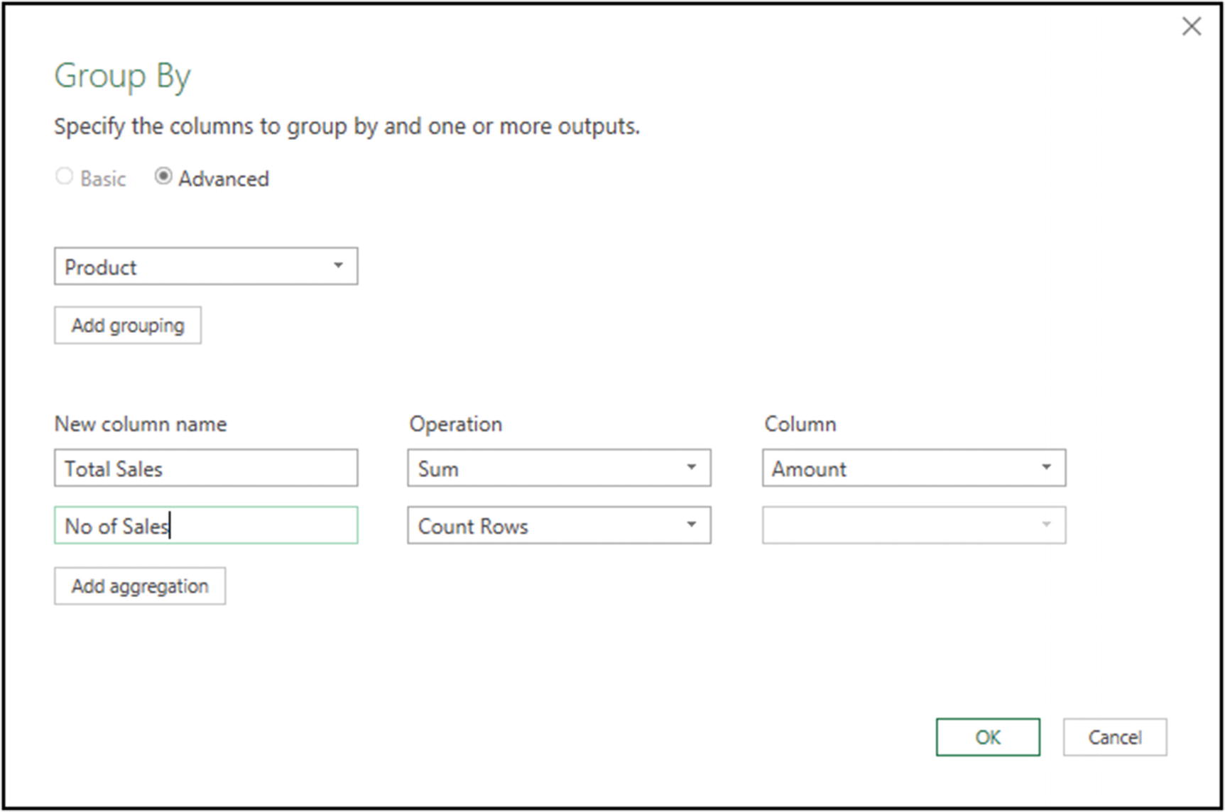
Group by product with sum and count rows aggregations
- 13.
Change the data type of the Total Sales column to Currency.
- 14.
Select the Total Sales column and click Home ➤ Sort Descending.
- 15.
Close and load the queries.
The tables are loaded onto separate sheets, but you can organize these how you want.
- 1.
Click Data ➤ Get Data ➤ Launch Power Query Editor.
- 2.
Select the Master query.
- 3.
Select the Source step in the Applied Steps box and click Home ➤ Refresh Preview.
The ProductSales and MonthlySalesByRegion tables are being picked up when combining all the workbook tables (Figure 5-59).
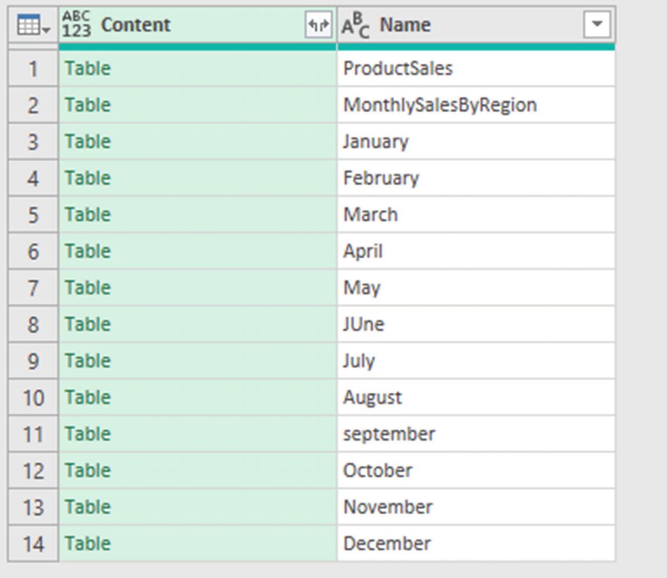
The report tables are recognized by Excel.CurrentWorkbook()
- 4.
Delete the current Filtered Rows step. We will insert a new one.
- 5.
Select the Source step and filter out the MonthlySalesByRegion and ProductSales tables from the Name column.
- 6.
Refresh the queries, and they work perfectly.
Power Query can also be used to create PivotTable-style reports.