Chapter 8

HJM Interest Rate Modeling with Two Risk Factors

In Chapters 6 and 7, we provided worked examples of how to use the yield curve simulation framework of Heath, Jarrow, and Morton (HJM) with two different assumptions about the volatility of forward rates. The first assumption was that volatility was dependent on the maturity of the forward rate and nothing else. The second assumption was that volatility of forward rates was dependent on both the level of rates and the maturity of forward rates being modeled. Both of these models were one-factor models, implying that random rate shifts are either all positive, all negative, or zero. This kind of yield curve movement is not consistent with the yield curve twists that are extremely common in the U.S. Treasury market and most other fixed income markets. In this chapter, we generalize the model to include two risk factors in order to increase the realism of the simulated yield curve.

PROBABILITY OF YIELD CURVE TWISTS IN THE U.S. TREASURY MARKET

In this chapter, we use the same data as inputs to the yield curve simulation process that we used in Chapters 6 and 7. A critical change in this chapter is to enhance our ability to model twists in the yield curve as shown in Exhibit 8.1.

EXHIBIT 8.1 Summary of U.S. Treasury Yield Curve Shifts Percentage Distribution of Daily Rate Shifts January 2, 1962, to August 22, 2011

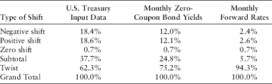
It shows that, for 12,386 days of movements in U.S. Treasury forward rates, yield curve twists occurred on 94.3 percent of the observations.

In order to incorporate yield curve twists in interest rate simulations under the Heath, Jarrow, and Morton (HJM) framework, we introduce a second risk factor driving interest rates in this chapter. The single-factor yield curve models of Ho and Lee (1986), Vasicek (1977), Hull and White (1990b), Black, Derman, and Toy (1990), and Black and Karasinski(1991) cannot model yield curve twists and, therefore, they do not provide a sufficient basis for interest rate risk management.

OBJECTIVES OF THE EXAMPLE AND KEY INPUT DATA

Following Jarrow (2002), we again make the same modeling assumptions for our worked example as in Chapters 6 and 7:

• Zero-coupon bond prices for the U.S. Treasury curve on March 31, 2011, are the basic inputs.
• Interest rate volatility assumptions are based on the Dickler, Jarrow, and van Deventer papers on daily U.S. Treasury yields and forward rates from 1962 to 2011. In this chapter, we retain the volatility assumptions used in Chapter 7 but expand the number of random risk factors driving interest rates to two factors.
• The modeling period is four equal length periods of one year each.
• The HJM implementation is that of a “bushy tree” that we describe below.

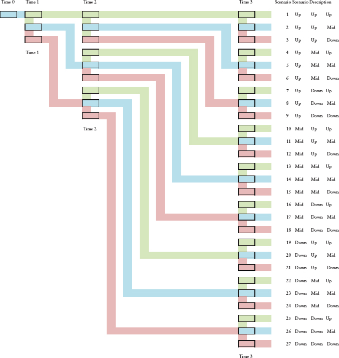
In Chapters 6 and 7, the HJM bushy tree that we constructed consisted solely of upshifts and downshifts because we were modeling as if only one random factor was driving interest rates. In this chapter, with two random factors, we move to a bushy tree that has upshifts, midshifts, and downshifts at each node in the tree, as shown in Exhibit 8.2. Please consider these terms as labels only, since forward rates and zero-coupon bond prices, of course, move in opposite directions.

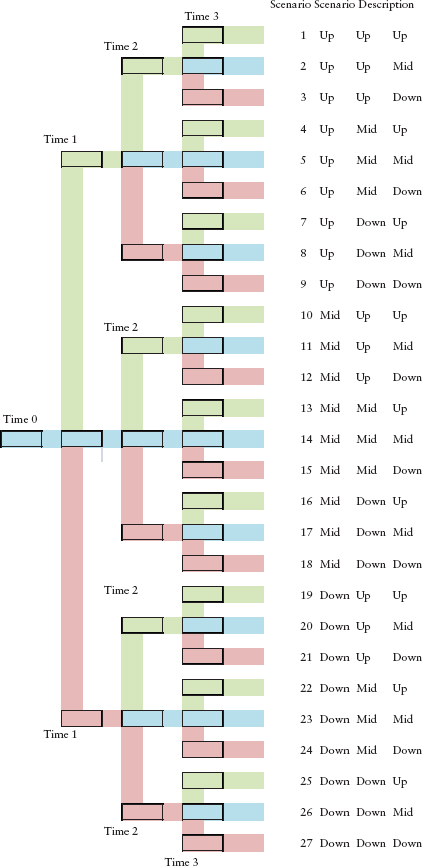
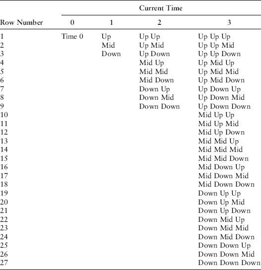
At each of the points in time on the lattice (time 0, 1, 2, 3, and 4) there are sets of zero-coupon bond prices and forward rates. At time 0, there is one set of data. At time one, there are three sets of data, the up-set, mid-set, and down-set. At time two, there are nine sets of data (up up, up mid, up down, mid up, mid mid, mid down, down up, down mid, and down down), and at time three there are 27 = 33 sets of data.

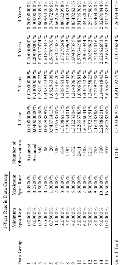
The table in Exhibit 8.3 shows the actual volatilities, resulting from all risk factors, for the one-year changes in continuously compounded forward rates from 1963 to 2011. This is the same data we used in Chapter 7. We use this table later to divide total volatility between two uncorrelated risk factors.

EXHIBIT 8.3 Standard Deviation of Annual Changes in One-Year Rate

We will again use the zero-coupon bond prices prevailing on March 31, 2011, as our other inputs.

Number of periods:	4
Length of periods (years)	1
Number of risk factors:	1
Volatility term structure:	Empirical, two factor

Period Start	Period End	Parameter Inputs Zero-Coupon Bond Prices
0	1	0.99700579
1	2	0.98411015
2	3	0.96189224
3	4	0.93085510

INTRODUCING A SECOND RISK FACTOR DRIVING INTEREST RATES

In the first two worked examples of the HJM approach in Chapters 6 and 7, the nature of the single factor that shocks one-year spot and forward rates was not specified. In this chapter, we take a cue from the popular academic models of the term structure of interest rates and postulate that one of the two factors driving changes in forward rates is the change in the short-run rate of interest. In the context of our annual model, the short rate is the one-year spot U.S. Treasury yield. For each of the one-year U.S. Treasury forward rates fk(t), we run the regression

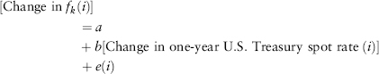
where the change in continuously compounded yields is measured over annual intervals from 1963 to 2011. The coefficients of the regressions for the one-year forward rates maturing in years 2, 3, . . ., 10 are as shown in Exhibit 8.4.

EXHIBIT 8.4 Regression Coefficients

Sources: Kamakura Corporation; Federal Reserve.

Dependent Variable	Coefficient b on 1-Year Change in 1-Year U.S. Treasury Rate	Standard Error of Regression
Forward 2	0.774288643	0.006547828
Forward 3	0.636076417	0.008161008
Forward 4	0.539780355	0.008511904
Forward 5	0.439882997	0.009330728
Forward 6	0.353383944	0.009567974
Forward 7	0.309579768	0.009585926
Forward 8	0.309049192	0.009148432
Forward 9	0.322513079	0.009361197
Forward 10	0.327367707	0.010036507

Graphically, it is easy to see that the historical response of forward rates to the spot rate of interest is neither constant—as assumed by Ho and Lee (1986)—nor declining, as assumed by Vasicek (1977) and Hull and White (1990b). Indeed, the response of the one-year forwards maturing in years 8, 9, and 10 years to changes in the one-year spot rate is larger than the response of the one-year forward maturing in year 7 as shown in Exhibit 8.5).

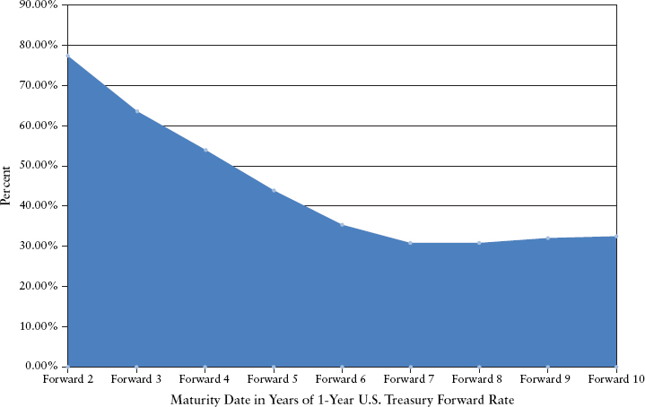
We use these regression coefficients to separate the total volatility (shown in the previous table) of each forward rate between two risk factors. The first risk factor is changes in the one-year spot U.S. Treasury. The second factor represents all other sources of shocks to forward rates.

Because of the nature of the linear regression of changes in one-year forward rates on the first risk factor, changes in the one-year spot U.S. Treasury rate, we know that risk factor 1 and risk factor 2 are uncorrelated. Therefore, total volatility for the forward rate maturing in T − t = k years can be divided as follows between the two risk factors:

We also know that the risk contribution of the first risk factor, the change in the spot one-year U.S. Treasury rate, is proportional to the regression coefficient αk of changes in forward rate maturing in year k on changes in the one-year spot rate. We denote the total volatility of the one-year U.S. Treasury spot rate by the subscript1, total:

This allows us to solve for the volatility of risk factor 2 using this equation:

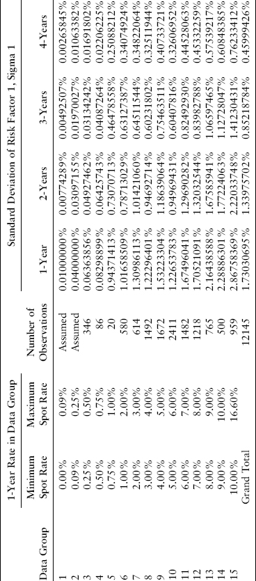
Because the total volatility for each forward rate varies by the level of the one-year U.S. Treasury spot rate, so will the values of σk,1 and σk,2. In one case (data group 6 for the forward rate maturing at time T = 3), we set the sigma for the second risk factor to zero and ascribed all of the total volatility to risk factor 1 because the calculated contribution of risk factor 1 was greater than the total volatility. In the worked example, we select the volatilities from lookup tables for the appropriate risk factor volatility. Using the previous equations, the look-up table for risk factor 1 (changes in the one-year spot rate) volatility is given in Exhibit 8.6.

EXHIBIT 8.6 Look-Up Table for Risk Factor 1

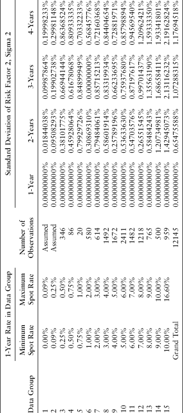
The lookup table for the general “all other” risk factor 2 is as shown in Exhibit 8.7.

EXHIBIT 8.7 Look-Up Table for General Risk Factor 2

KEY IMPLICATIONS AND NOTATION OF THE HJM APPROACH

We now reintroduce a slightly modified version of the notation used in Chapters 6 and 7:

Δ	= length of time period, which is 1 in this example
r(t, st)	= the simple one-period, risk-free interest rate as of current time t in state st
R(t, st)	= 1 + r(t, st), the total return, the value of $1 dollar invested at the risk-free rate for 1 period
f(t, T, st)	= the simple one-period forward rate maturing at time T in state st as of time t
F(t, T, st)	= 1 + f(t, T, st), the return on $1 invested at the forward rate for one period
σ1 (t, T, st)	= forward rate volatility due to risk factor 1 at time t for the one-period forward rate maturing at T in state st (a sequence of ups and downs). Because σ1 is dependent on the spot U.S. Treasury rate, the state st is very important in determining its level.
σ2 (t, T, st)	= forward rate volatility due to risk factor 2 at time t for the one-period forward rate maturing at T in state st (a sequence of ups and downs). Because σ2 is dependent on the spot U.S. Treasury rate, the state st is very important in determining its level.
P(t, T, st)	= zero-coupon bond price at time t maturing at time T in state st (i.e., up or down)
Index(1)	An indicator of the state for risk factor 1, defined below
Index(2)	An indicator of the state for risk factor 2, defined below
K(i, t, T, st)	= the sum of the forward volatilities for risk factor i (either 1 or 2) as of time t for the 1-period forward rates from t + Δ to T, as shown here:

Note that this is a slightly different definition of K than we used in Chapters 6 and 7.

We again use the trigonometric function cosh(x):

We again arrange the tree to look like a table by stretching the bushy tree as in Exhibit 8.8.

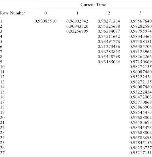
A completely populated zero-coupon bond price tree would then be summarized like this; prices shown are for the zero-coupon bond price maturing at time T = 4 at times 0, 1, 2, and 3 as shown in Exhibit 8.9.

EXHIBIT 8.9 Four-Year, Zero-Coupon Bond Price

The mapping of the sequence of up and down states is shown in Exhibit 8.10, consistent with the stretched tree in Exhibit 8.8.

EXHIBIT 8.10 Map of Sequence of States

In order to populate the trees with zero-coupon bond prices and forward rates, we again need to select the relevant pseudo-probabilities.

PSEUDO-PROBABILITIES

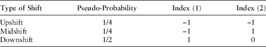
Consistent with Chapter 7 of Jarrow (2002), and without loss of generality, we set the probability of an upshift to one-fourth, the probability of a midshift to one-fourth, and the probability of a downshift to one-half. The no-arbitrage restrictions that stem from this set of pseudo-probabilities are given next.

The Formula for Zero-Coupon Bond Price Shifts with Two Risk Factors

In Chapters 6 and 7, we used equation 15.17 in Jarrow (2002, 286) to calculate the no-arbitrage shifts in zero-coupon bond prices. Alternatively, when there is one risk factor, we could have used equation 15.19 in Jarrow (2002, 287) to shift forward rates and derive zero-coupon bond prices from the forward rates. Now that we have two risk factors, it is convenient to calculate the forward rates first. We do this using equations 15.32, 15.39a, and 15.39b in Jarrow (2002, 293–296). We use this equation for the shift in forward rates:

(8.1)

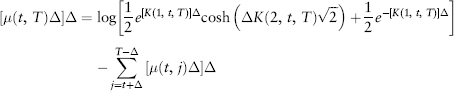
Where when T = t + Δ, the expression μ becomes

We use this expression to evaluate equation (8.1) when T > t + Δ:

The values for the pseudo-probabilities and Index (1) and Index (2) are set as follows:

Building the Bushy Tree for Zero-Coupon Bonds Maturing at Time T = 2

We now populate the bushy tree for the two-year, zero-coupon bond. We calculate each element of equation (8.1). When t = 0 and T = 2, we know Δ = 1 and

The one-period risk-free return (1 plus the risk-free rate) is again

The one-period spot rate for U.S. Treasuries is r(0, st) = R(0, st) −1 = 0.3003206 percent. At this level of the spot rate for U.S. Treasuries, volatilities for risk factor 1 are selected from data group 3 in the look-up table above. The volatilities for risk factor 1 for the one-year forward rates maturing in years 2, 3, and 4 are 0.000492746, 0.000313424, and 0.00016918. The volatilities for risk factor 2 for the one-year forward rates maturing in years 2, 3, and 4 are 0.003810177, 0.006694414, and 0.008636852.

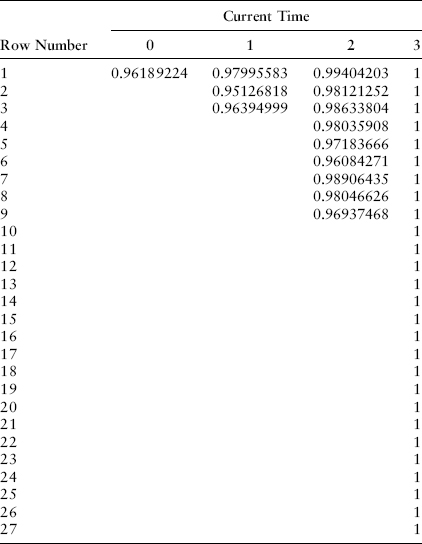
The scaled sum of sigmas K(1, t, T, st) for t = 0 and T = 2 becomes

and, therefore,

Similarly,

We also can calculate that

Using formula (8.1) with these inputs and the fact that the variable Index(1) = −1 and Index (2) = −1 for an upshift gives us the forward returns for an upshift, midshift, and downshift as follows: 1.007170561, 1.018083343, and 1.013610665. From these we calculate the zero-coupon bond prices:

For a midshift, we set Index (1) = −1 and Index (2) = +1 and calculate

For a downshift, we set Index (1) = 1 and Index (2) = 0 and recalculate formula 1 to get

We have fully populated the bushy tree for the zero-coupon bond maturing at T = 2 (note values have been rounded for display only), since all the up-, mid- and downstates at time t = 2 result in a riskless payoff of the zero-coupon bond at its face value of 1 as shown in Exhibit 8.11.

EXHIBIT 8.11 Two-Year, Zero-Coupon Bond Price

Building the Bushy Tree for Zero-Coupon Bonds Maturing at Time T = 3

For the zero-coupon bonds and one-period forward returns (= 1 + forward rate) maturing at time T = 3, we use the same volatilities listed above for risk factors 1 and 2 to calculate

The resulting forward returns for an upshift, midshift, and downshift are 1.013189027, 1.032556197, and 1.023468132. Zero-coupon bond prices are calculated from the one-period forward returns, so

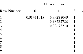
The zero-coupon bond prices for an upshift, midshift, and downshift are 0.979956, 0.951268, and 0.963950. To eight decimal places, we have populated the second column of the zero-coupon bond price table for the zero-coupon bond maturing at T = 3 as shown in Exhibit 8.12.

EXHIBIT 8.12 Three-Year, Zero-Coupon Bond Price

Building the Bushy Tree for Zero-Coupon Bonds Maturing at Time T = 4

We now populate the bushy tree for the zero-coupon bond maturing at T = 4. Using the same volatilities as before for both risk factors 1 and 2, we find that

Using formula (8.1) with the correct values for Index (1) and Index (2) leads to the following forward returns for an upshift, midshift, and downshift: 1.020756042, 1.045998862, and 1.033650059. The zero-coupon bond price is calculated as follows:

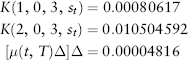
This gives us the three zero-coupon bond prices of the column labeled 1 in this table for up-, mid-, and downshifts: 0.96002942, 0.90943520, and 0.93256899 as shown in Exhibit 8.13.

EXHIBIT 8.13 Four-Year, Zero-Coupon Bond Price

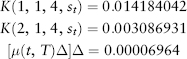
Now, we move to the third column, which displays the outcome of the T = 4 zero-coupon bond price after nine scenarios: up up, up mid, up down, mid up, mid mid, mid down, down up, down mid, and down down. We calculate P(2, 4, st = up), P(2, 4, st = mid), and P(2, 4, st = down) after the initial down state as follows. When t = 1, T = 4, and Δ = 1 then the volatilities for the two remaining one-period forward rates that are relevant are taken from the look-up table for data group 6 for risk factor 1: 0.007871303 and 0.006312739. For risk factor 2, the volatilities for the two remaining one-period forward rates are also chosen from data group 6: 0.003086931 and 0. The zero value was described previously; the implied volatility for risk factor 1 was greater than measured total volatility for the forward rate maturing at T = 3 in data group 6, so the risk factor 1 volatility was set to total volatility and risk factor 2 volatility was set to zero.

At time 1 in the downstate, the zero-coupon bond prices for maturities at T = 2, 3, and 4 are 0.986572, 0.963950, and 0.932569. We make the intermediate calculations as previously for the zero-coupon bond maturing at T = 4:

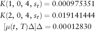
We can calculate the values of the one-period forward return maturing at time T = 4 in the upstate, midstate, and downstate as follows: 1.027216983, 1.027216983, and 1.040268304. Similarly, using the appropriate intermediate calculations, we can calculate the forward returns for maturity at T = 3: 1.011056564, 1.01992291, and 1.031592858. Since

the zero-coupon bond prices for maturity at T = 4 in the down up, down mid, and down down states are as follows:

We have correctly populated the seventh, eighth, and ninth rows of column 3 (t = 2) of the previous bushy tree for the zero-coupon bond maturing at T = 4 (note values have been rounded to six decimal places for display only). The remaining calculations are left to the reader.

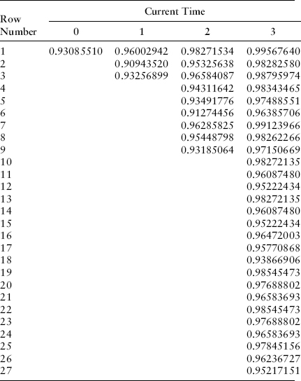
If we combine all of these tables, we can create a table of the term structure of zero-coupon bond prices in each scenario as in examples one and two. The shading highlights two nodes of the bushy tree where values are identical because of the occurrence of σ2 = 0 at one point on the bushy tree as shown in Exhibit 8.14.

EXHIBIT 8.14 Zero-Coupon Bond Prices

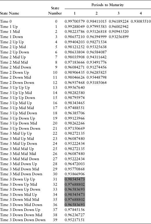
At any point in time t, the continuously compounded yield to maturity at time T can be calculated as y(T − t) = −ln[P(t,T)]/(T − t). Note that we have no negative rates on this bushy tree and that yield curve shifts are much more complex than in the two prior examples using one risk factor as shown in Exhibit 8.15.

EXHIBIT 8.15 Continuously Compounded Zero-Coupon Yields

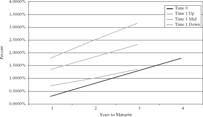
We can graph yield curve movements as shown in Exhibit 8.16 at time t = 1. We plot yield curves for the up-, mid-, and downshifts. These shifts are relative to the one-period forward rates prevailing at time zero for maturity at time T = 2 and T = 3. Because these one-period forward rates were much higher than yields as of time t = 0, all three shifts produce yields higher than time-zero yields.

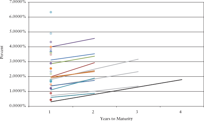
When we add nine yield curves prevailing at time t = 3 and 27 single-point yield curves prevailing at time t = 4, two things are very clear. First, yield curve movements in a two-factor model are much more complex and much more realistic than what we saw in the two one-factor examples. Second, in the low-yield environment prevailing as of March 31, 2011, no arbitrage yield curve simulation shows “there is nowhere to go but up” from a yield curve perspective as shown in Exhibit 8.17.

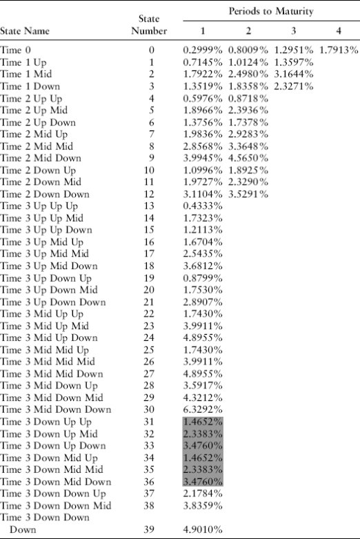
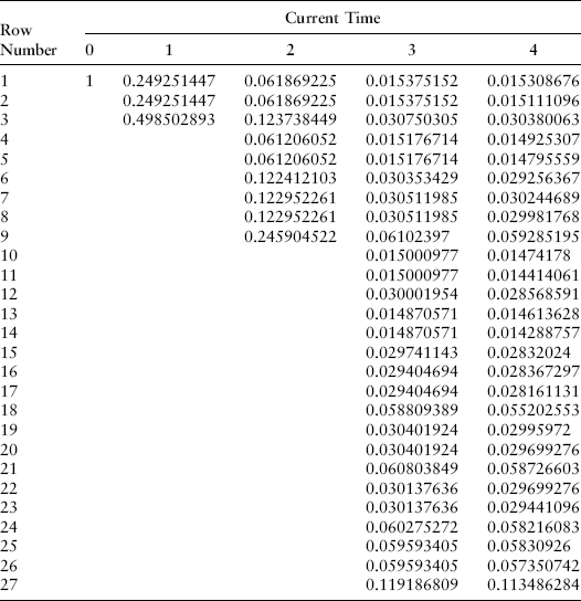
Finally, we can display the one-year U.S. Treasury spot rates and the associated term structure of one-year forward rates in each scenario as shown in Exhibit 8.18.

EXHIBIT 8.18 One-Year Forward Rates, Simple Interest

VALUATION IN THE HJM FRAMEWORK

Jarrow, as quoted in Chapter 6, described valuation as the expected value of cash flows using the risk-neutral probabilities. Note that column 1 denotes the riskless one-period interest rate in each scenario. For the scenario number 39 (three consecutive downshifts in zero-coupon bond prices), cash flows at time T = 4 would be discounted by the one-year spot rates at time t = 0, by the one-year spot rate at time t = 1 in scenario 3 (down), by the one-year spot rate in scenario 12 (down down) at time t = 2, and by the one-year spot rate at time t = 3 in scenario 39 (down down down). The discount factor is

These discount factors are displayed in Exhibit 8.19 for each potential cash flow date.

EXHIBIT 8.19 Discount Factors

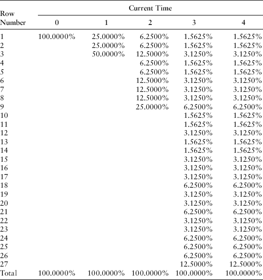
When taking expected values, we can calculate the probability of each scenario coming about since the probabilities of an upshift, midshift, and downshift are 1/4, 1/4, and 1/2 as shown in Exhibit 8.20.

EXHIBIT 8.20 Probability of Each State

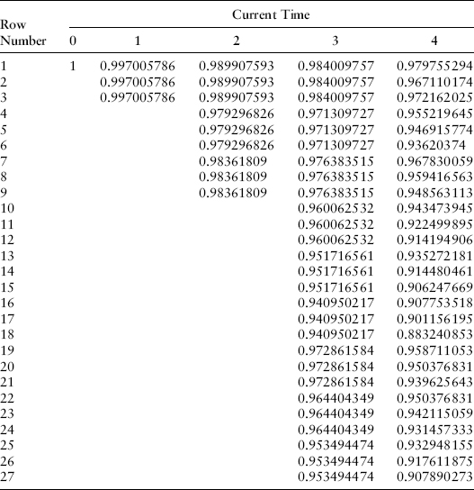
It is again convenient to calculate the probability-weighted discount factors for use in calculating the expected present value of cash flows as shown in Exhibit 8.21.

EXHIBIT 8.21 Probability-Weighted Discount Factors

We now use the HJM bushy trees we have generated to value representative securities.

VALUATION OF A ZERO-COUPON BOND MATURING AT TIME T = 4

A riskless zero-coupon bond pays $1 in each of the 27 nodes of the bushy tree that prevail at time T = 4 as shown in Exhibit 8.22.

EXHIBIT 8.22 Maturity of Cash Flow Received

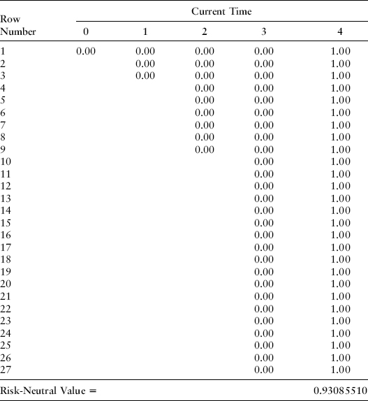
When we multiply this vector of 1s times the probability-weighted discount factors in the time T = 4 column in the previous table in Exhibit 8.22 and add them, we get a zero-coupon bond price of 0.93085510, which is the value we should get in a no-arbitrage economy, the value observable in the market and used as an input to create the tree.

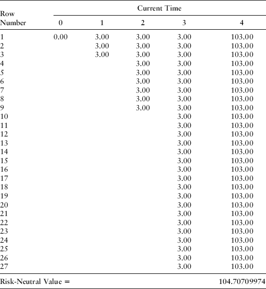
VALUATION OF A COUPON-BEARING BOND PAYING ANNUAL INTEREST

Next we value a bond with no credit risk that pays $3 in interest at every scenario at times T = 1, 2, 3, and 4 plus principal of 100 at time T = 4. The valuation is calculated by multiplying each cash flow by the matching probability-weighted discount factor, to get a value of 104.70709974. It will again surprise many that this is the same value that we arrived at in Chapters 6 and 7, even though the volatilities used and the number of risk factors used are different. The values are the same because, by construction, our valuations for the zero-coupon bond prices at time zero for maturities at T = 1, 2, 3, and 4 continue to match the inputs. Multiplying these zero-coupon bond prices times 3, 3, 3, and 103 also leads to a value of 104.70709974 as it should as shown in Exhibit 8.23.

EXHIBIT 8.23 Maturity of Cash Flow Received

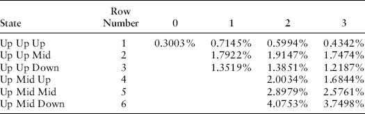
VALUATION OF A DIGITAL OPTION ON THE ONE-YEAR U.S. TREASURY RATE

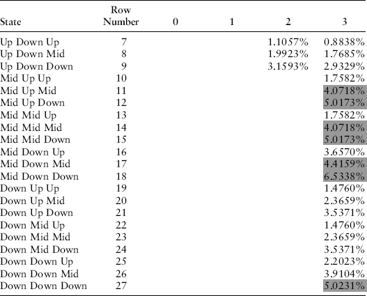
Now, we value a digital option that pays $1 at time T = 3 if (at that time) the one-year U.S. Treasury rate (for maturity at T = 4) is over 4 percent. If we look at the table of the term structure of one-year spot rates over time, this happens at the seven shaded scenarios out of 27 possibilities at time t = 3 as shown in Exhibit 8.24.

EXHIBIT 8.24 Spot Rate Process

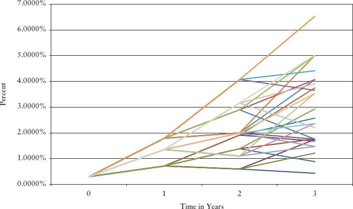
The evolution of the spot rate can be displayed graphically as in Exhibit 8.25.

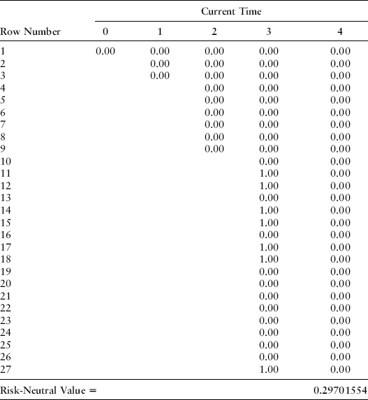
The cash flow payoffs in the seven relevant scenarios can be input in Exhibit 8.26 and multiplied by the probability weighted discount factors to find that this option has a value of 0.29701554 as shown in the exhibit.

EXHIBIT 8.26 Maturity of Cash Flow Received

REPLICATION OF HJM EXAMPLE 3 IN COMMON SPREADSHEET SOFTWARE

The readers of this book are almost certain to be proficient in the use of common spreadsheet software. In replicating the examples in this and other chapters, any discrepancy in values within the first 10 decimal places is most likely an error by the analyst or, heaven forbid, the authors. In the construction of the examples in this book, every discrepancy in the first 10 decimal places has been an error, not the normal computer science rounding error that the authors would typically blame first as the cause.

CONCLUSION

This chapter, continuing the examples of Chapters 6 and 7, shows how to simulate zero-coupon bond prices, forward rates, and zero-coupon bond yields in an HJM framework with two risk factors and rate-dependent and maturity-dependent interest rate volatility. The results show a rich twist in simulated yield curves and a pull of rates upward from a very low rate environment. Monte Carlo simulation, an alternative to the bushy tree framework, can be done in a fully consistent way. We discuss that in detail in Chapter 10.

In the next chapter, we introduce a third risk factor to further advance the realism of the model.