
Chapter 22
Forward and Futures Contracts
In this chapter, we continue the process of valuing the most common instruments on the balance sheet of major financial institutions around the world. Valuation enables us to efficiently perform a multiperiod simulation of cash flows and future values for these instruments, both of which are critical to the ultimate objective—measuring interest rate risk, market risk, liquidity risk, and credit risk in a consistent framework via the Jarrow-Merton put option introduced in Chapter 1.
Our focus in this chapter is on forward contracts and futures contracts for interest rate–related instruments. Careful attention to this issue is important both from a correct hedging analysis and from an accounting perspective. This chapter lays the groundwork for the correlation requirements of those standards, both in terms of valuation and cash flow. In Chapter 20, we warned of the dangers of collusion and market manipulation in the market for credit default swaps. (In Chapter 17, on credit spread modeling, we mentioned the legal actions alleging similar manipulation in the LIBOR market. On June 27, 2012, agencies of the U.S. government and the UK’s Financial Services Authority levied more than $450 million in penalties for LIBOR manipulation against Barclays PLC.) We assume perfectly competitive markets in the following analysis, but we warn readers, as we have throughout this volume, to make the appropriate adjustments given the nature of the pricing index and the nature of the counterparty. It is a mistake to assume that (1) everyone you trade with is Mother Teresa and that (2) you are the smartest one in the room. Lehman veteran Larry McDonald is often quoted as saying “If you are playing poker and you can’t find the sucker at the table, it’s probably you.” Beware.
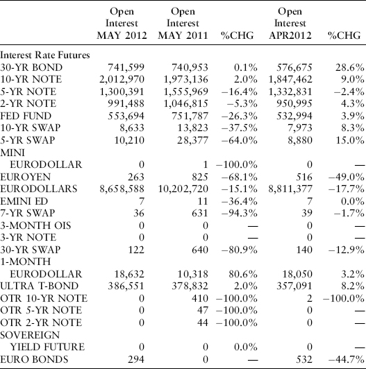
Financial forward and futures contracts are critical everyday tools of risk management and investment management. Their popularity is probably best summarized by the interest rate futures contracts traded on the Chicago Mercantile Exchange. Open interest in these contracts has long exceeded trillions of dollars, even for the most long-dated contracts. Eurodollar futures on June 28, 2012, traded at maturities as long as nine years forward. Exhibit 22.1 from the CME Group summarizes the open interest in interest rate futures as of May 2012.
EXHIBIT 22.1 CME Group Exchange Open Interest Report—Monthly
Source: www.cmegroup.com/wrappedpages/web_monthly_report/Web_OI_Report_CMEG.pdf.
This chapter illustrates the important distinctions between forward and futures contracts of different types, using the tools of Chapter 21 that we developed in the context of valuing options on zero-coupon and coupon-bearing bonds. Note that we don’t delve into the detailed contract specifications of specific futures contracts because the information is overwhelmingly voluminous. Instead, we concentrate on analytical methods that can be applied to any forward or futures contract with appropriate adjustments for the details of the instrument. Daily cash flows and margin requirements are critical considerations with interest rate futures. We use the three-factor Heath, Jarrow, and Morton (HJM) bushy tree from Chapter 9 again in this chapter for ease of exposition. In practice, we would use daily time steps and a Monte Carlo implementation of the HJM bushy tree. We start first with various forward contracts and then cover futures contracts.
FORWARD CONTRACTS ON ZERO-COUPON BONDS
The most basic forward contract is a forward contract on the price of a zero-coupon bond. In this section and the rest of the chapter, we need to make an important distinction between the value of an existing contract on the books of an investment manager, insurance firm, or bank and the price of the forward contract quoted in the market. Before making this distinction clear, a real-world example of a forward contract on zero-coupon bonds is useful. In this case, the best example is provided by the 90-day bank bill futures contract traded on the Sydney Futures Exchange. For purposes of this section, we ignore daily mark-to-market requirements and analyze this contract as a forward, not a futures, contract. (We perform the true futures analysis later in the chapter.) Our example has the following criteria:
Valuation formula:
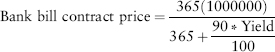
The bank bill contract assumes the underlying instrument pays simple interest on an actual/365-day basis and has a maturity of 90 days. Essentially, the price of the contract is the price of a 90-day zero-coupon bond with principal amount in Australian dollars of A$1 million at maturity. The calculation is the same as those we used in Chapter 4. One of the key features of the Sydney Bank Bill contract, as opposed to the Eurodollar contracts we will discuss, is that the value of a 0.01 percent change in yield depends on the level of interest rates rather than being a constant dollar amount like the Eurodollar contract:
| Yield (%) | A$ Value of 0.01% Yield Increase |
| 9.00% | A$23.60 |
| 10.00% | A$23.49 |
| 11.00% | A$23.37 |
| 12.00% | A$23.26 |
Note that the quotation method (100 − Yield) is irrelevant to valuation—only the underlying cash flow described by the valuation formula matters for valuation purposes.
For notational convenience, we do the valuation analysis assuming that the principal amount on the underlying instrument is A$1 instead of A$1 million. We know from Chapter 4 that the forward price of this bond in a no-arbitrage world with perfect competition should be the ratio of zero-coupon bond prices:
![]()
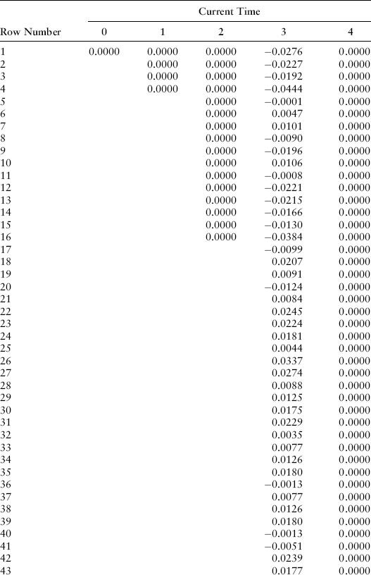
where T2 is the maturity date of the underlying instrument (in years), T1 is the maturity date of the forward contract, and t is the current time. This result doesn’t depend on any particular term structure model since it can be derived using arbitrage arguments alone. If a financial institution has bought the forward contract at an exercise price of K, then at the maturity of the forward (time T = T1), the gain will be P(r,T1,T2) − K. Let’s assume that the forward contract we are analyzing is a three-year forward contract on the one-year zero-coupon bond maturing at time T = 4. We can use the bushy tree of Chapter 9 and the related one-year zero-coupon bond prices as of time T = 3 to analyze cash flows to the purchaser of the forward contract for any given exercise price K. For an exercise price K = 0.97, the cash flows at time T = 3 on the 64 nodes are shown in Exhibit 22.2.
EXHIBIT 22.2 Gain or Loss on Three-Year Forward Contract on Zero-Coupon Bond Maturing in Year 2
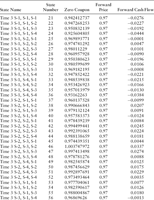
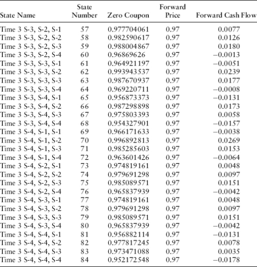
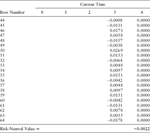
If we drop these cash flows into the cash flow table and multiply by the proper probability-weighted discount factors, we find in Exhibit 22.3 that the value of this forward position is −0.0022.
EXHIBIT 22.3 Maturity of Cash Flow Received
We know, however, that we can replicate the cash flows of this forward contract by making these transactions:
We can confirm that, indeed,
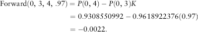
This result stems from no-arbitrage arguments and holds for any term structure model. Leaving aside the existing forward contract purchased for K = 0.97, what should the exercise price K of a new forward contract be today? Since no initial cash is necessary to buy a forward at market, the value of the forward should be zero so that
![]()
or
![]()
We can confirm this result by using the HJM cash flow table and solving for the level of K that makes the value of the existing futures contract zero.
Turning back to the Sydney forward contract, the observable market price (in zero-coupon bond terms) equals the forward bond price. In yield terms, as quoted on the Sydney Futures Exchange, the quoted yield will be
![]()
Later in this chapter, we deal with the implications of daily margin requirements and the possibility that there could be a default (1) either by the Exchange itself or (2) on the instrument underlying the forward contract in keeping with our interest in an integrated treatment of interest rate risk, market risk, liquidity risk, and credit risk. The analysis in this section implicitly assumes that both the Exchange and the underlying instrument are default free.
Forward Rate Agreements
The design of the Sydney Futures Exchange Bank Bill Contract is one of a relatively small number of contracts where the underlying instrument is a zero-coupon bond. It is most common for the underlying instrument to be expressed in terms of an interest rate. Perhaps the most common forward contract with this structure is the forward rate agreement (FRA), where the counterparties agree on a strike rate K at maturity T1 based on an underlying rate for an instrument maturing at T2. The cash flow at time T2 from the FRA is proportional to the FRA rate at maturity and the strike rate K:
![]()
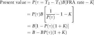
where the coefficient B reflects the notional principal amount, the maturity of the underlying instrument, and the interest quotation method used for the FRA contract (i.e., actual/360 days, actual/365 days, etc.). In this section, we analyze the case where this interest differential is paid at the maturity of the underlying instrument, T2. Conventional FRAs normally pay in an economically equivalent way, paying the present value of this interest rate differential at the maturity of the FRA contract, T1.
We value the contract as if cash flowed at time T1 by taking the simple present value of T2 cash flow from the perspective of time T1 (the standard FRA convention):
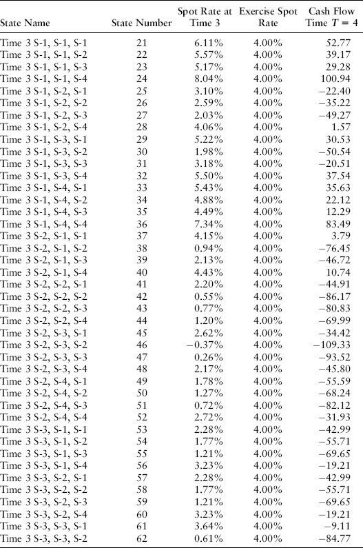
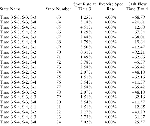
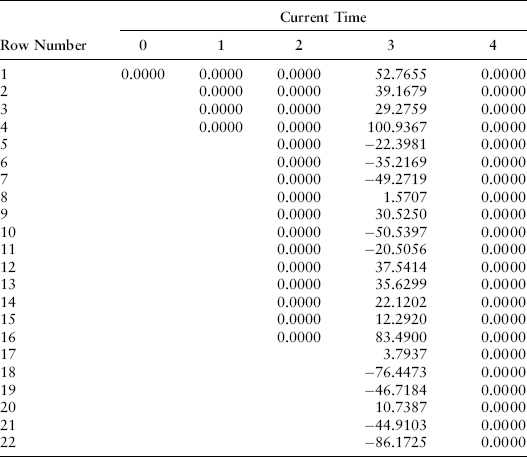
Let’s assume that B is A$25 per 1 percent rate change (A$0.25 per basis point) and that the FRA exercise price is K = 4 percent. You receive any excess of the actual spot rate over 4 percent and you pay any shortfall of the actual spot rate under 4 percent. The cash flows that are paid at time T = 4 on a one-year underlying FRA are set out in Exhibit 22.4 for each of the relevant 64 nodes.
EXHIBIT 22.4 FRA at 4 Percent on One-Year Instrument
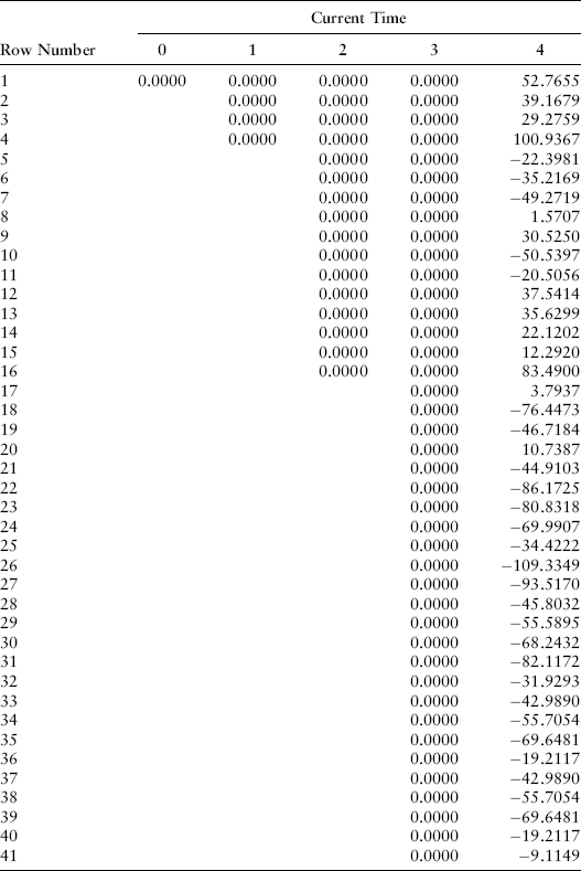
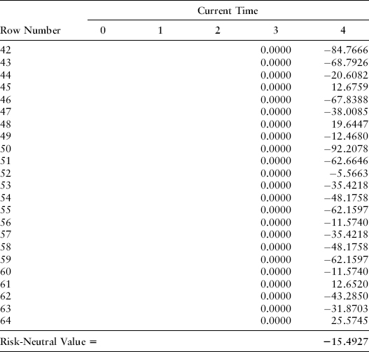
If we drop these into the cash flow table, we get the value −15.4927 in Exhibit 22.5.
EXHIBIT 22.5 Maturity of Cash Flow Received
Note that we can replicate the net present value that will be received under this transaction at time T = 3. We know B = A$2,500 (since rates are expressed as a decimal) and the FRA exercise price is 0.04. We replicate this time T = 3 net present value payoff with the following steps:
No arbitrage requires that the net cost of this strategy be the same as −15.4927 and we can confirm that is the case:
![]()
We can also solve for the implied “price” of new FRA transactions K, recognizing that an FRA transaction at time zero is costless and therefore should have a value of zero to avoid arbitrage possibilities:
![]()
Again, this formula holds for any term structure model because the replication of the FRA is independent of the term structure model selected. What if the rate differential between the FRA rate and K is paid on an undiscounted basis at time T1? We answer that question in the next section.
EURODOLLAR FUTURES-TYPE FORWARD CONTRACTS
What if the market convention regarding FRA payment was that the forward rate agreement pays its cash flow:
![]()
at the T1 maturity of the FRA contract instead its present value at time T1 or payment in cash at the T2 maturity of the underlying instrument? An FRA that pays in this manner is essentially equivalent to a Eurodollar Futures contract with no mark-to-market margin (i.e., a Eurodollar futures-type forward). Such a Eurodollar futures-type forward, if modeled after the Chicago Mercantile Exchange Eurodollar futures contract, would pay $25 for every one basis point differential between the settlement yield on the futures-type forward and the strike price. Unlike the Sydney Futures Exchange Bank Bill future discussed in the previous section, the dollar value of a basis point change in quoted yield is the same for all levels of interest rates under this type of contract. The cash flow at time T1 under this kind of contract is
![]()
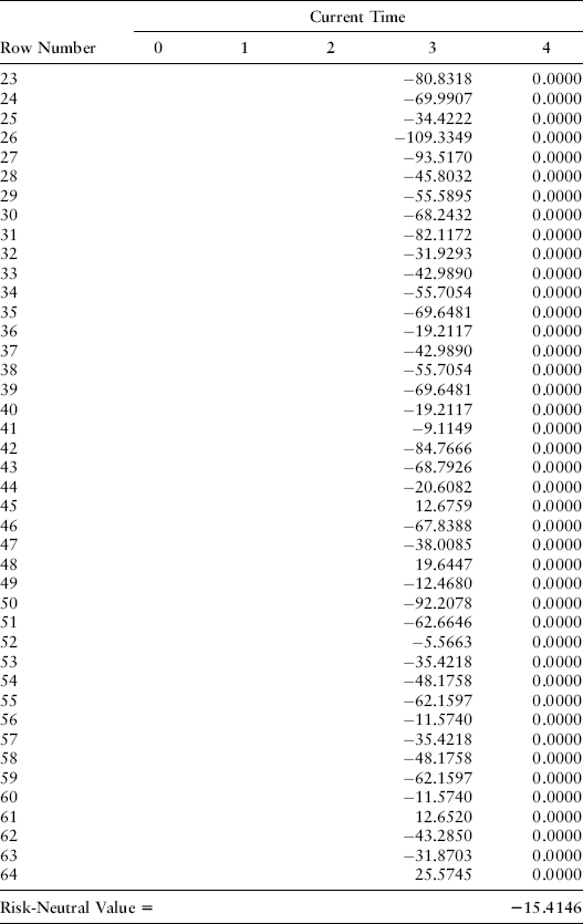
The cash flows are the same as before but they arrive at time T = 3 instead of time T = 4. We can calculate the value of this kind of structure by dropping the cash flows into a different column, the column for time T = 3, in the cash flow table. The value is −15.4146, as shown in Exhibit 22.6.
EXHIBIT 22.6 Maturity of Cash Flow Received
The valuation formulas for this instrument are more complex than the simple no-arbitrage results given previously.
FUTURES ON ZERO-COUPON BONDS: THE SYDNEY FUTURES EXCHANGE BANK BILL CONTRACT
From this point on in the chapter, we deal with true futures contracts. A true futures contract has daily mark-to-market requirements, with cash flow on an existing contract occurring continuously through its life. Ending cash flow is essentially zero, since the full amount of the change in observable futures prices over the life of the contract will have already been paid in cash through the continuous mark-to-market requirements. We will ignore initial margin payments and the return of these initial payments since they represent a simple zero-coupon bond-type adjustment to the formulas that follow.
Like the previous three sections, there is an important distinction between the market value of an existing futures position V and the observable market price of a futures contract Q. The first three sections showed the distinct differences between V and Q for three different types of forward contracts. In this section and the remainder of the chapter, we note the following:
- The market value V of an existing futures position will always be zero since (1) the market price of a new futures contract must be zero to avoid arbitrage and (2) a previously taken futures position is continuously made equivalent to a new position by continuous margin payments. The observable market price Q of the future contract and the initial strike rate K on the futures transaction, put in place at time t0, are related by the fact that cash payments of at least M = K − Q, the cumulative net loss (gain) on the futures contract, must have been made to (withdrawn from) the margin account since initiation of the transaction at time t0. The balance of the margin account is unknown since parties with a positive margin balance may use the cash proceeds for any purpose.
- This important comment notwithstanding, a trader is always thinking about their gains or losses in terms of the original rate at which the futures contract was purchased K and the current market price Q. It is critical to note that this differential will have already impacted the financial institution’s balance sheet (i.e., the cash account) and the trader’s focus on the differential K − Q reflects only a partial view of the impact of the futures contract on the institution. Most sophisticated institutions are taking both views of the impact of a futures contract, the trader’s view and the true daily cash flow pattern via the margin accounts.
These comments require a careful vocabulary to bridge the gap between the jargon of market participants and financial reality. To a market participant, the value of a futures contract is Q − K, even though the margin account balance would be Max(0,K − Q) rather than always being Q − K. These same market participants are rarely aware of the margin account balance, which is normally managed by an operational group. To a financial economist, the value is zero. Fortunately, the interest rate risk of a futures position to both groups is the change in Q that results from a change in interest rates, as captured by movements in the single stochastic factor r (if the Vasicek term structure model applies) or by movements in the three factors driving our HJM model from Chapter 9. Taking care to remember this distinction between viewpoints, we ignore the market value of an existing futures position V and concentrate on determining the observable market price Q.1
In modeling interest rate futures contracts, the most important difference versus the forward rate contracts discussed earlier in the chapter is easy to summarize. Let’s assume at time T = 0 one takes a position in a futures contract maturing at time T = 3 on the zero-coupon bond maturing at time T = 4. Obviously, at time T = 3, the price of the maturing futures contract will be forced by arbitrage to exactly equal the time T = 3 price of the zero-coupon bond maturing at time T = 4. This boundary condition is no different than it is for forward contracts. The difference comes in what happens at times T = 1 and T = 2. In the case of a forward contract maturing at time T = 3, nothing happens at times 1 and 2, which is why the cash flows above were zero for those time periods. We write the price of a futures contract as of time t with maturity at T = 3 on the zero-coupon bond maturing at T = 4 as F(t,3,4). The time zero price of the futures contract is F(0,3,4). At time 1, there are four nodes on the bushy tree and the futures price will be taken on one of four values, F(1,3,4,si) for i = 1, 2, 3, and 4. At each of these four nodes, there will be cash flow equal to F(1,3,4,si) − F(0,3,4). This cash flow either represents the withdrawal of a gain from a margin account or the contribution of a loss back into the margin account. After this cash flow has occurred at time T = 1, of course, an existing futures position and a new futures position are identical. Both have zero dollars in the margin account.
At time T = 2, there are 16 nodes and there will be 16 gains or losses on the futures position relative to the four futures values on the nodes at T = 1.
The analytical derivation of the futures price evolution is nicely done by Chen (1992) in the Vasicek framework. As the number of risk factors driving interest rates in an HJM framework gets larger and larger for greater realism, futures prices and their evolution in general can be most usefully derived by numerical methods. See Jarrow and Turnbull (1996) for an excellent summary of the general principles that govern the evolution of futures prices. The need for numerical methods is particularly true in light of the “cheapest to deliver option” embedded in many bond futures contracts. We turn to that issue now.
FUTURES ON COUPON-BEARING BONDS: DEALING WITH THE CHEAPEST TO DELIVER OPTION
In this section, we consider the contract specifications of the Singapore Exchange’s Japanese government bond (JGB) contract. Let’s assume the coupon rate on the futures contract is 2 percent:
In actual operation, there will be a number of JGB issues that are deliverable under the Singapore contract. The seller of the futures contract has a delivery option which allows the seller of the futures contract to deliver the cheapest bond if the seller of the futures contract chooses to hold the contract to maturity. If there are N deliverable bonds, the exchange will calculate a delivery factor Fi, which specifies the ratio of the principal amount on the ith deliverable bond to the notional principal of ¥50,000,000 that is necessary to satisfy delivery requirements.
One of the bonds at any given time is the cheapest to deliver. After multiplying the yen coupon amounts and yen principal amount on this bond times the delivery factor, we will have the j maturities and cash flow amounts underlying the bond future. The market price of the bond future (as long as only one bond is deliverable) is the sum of zero-coupon bond futures prices (assuming one yen of principal on each zero-coupon bond future) times these cash flow amounts Ci:
![]()
T0 is the maturity date of the bond futures contract. The sensitivity analysis of bond futures, assuming only one bond is deliverable, is the sum of the sensitivities for the zero-coupon bond futures portfolio, which replicates the cash flows on the bond.
What about the value of the delivery option? Let us assume that there are two deliverable bonds and the one-factor Vasicek model is a realistic description of rate movements. (Model Risk Alert: It is not realistic.) Using the insights of Jamshidian’s (1989) approach to coupon-bearing bond options valuation, we know that there will be a level of the short rate r, which we label s*, such that the two bonds are equally attractive to deliver as of time Tf. Above s*, bond one is cheaper to deliver. Below s*, bond two is cheaper to deliver. We can solve the partial differential equation for futures valuation subject to the boundary conditions that the futures price converges to bond one’s deliverable value above s* and to bond two’s deliverable value below s*. We also impose the condition that the first and second derivatives of the futures price are smooth at a short rate level of s*. The result is a special weighted average of the futures prices that would have prevailed if each bond was the only deliverable bond under the futures contract. There are other options embedded in common U.S. and Japanese bond contracts that can be analyzed in a related way. The process is much more complex in a realistic HJM framework with the 5 to 10 risk factors that we showed were necessary for realism in Chapter 3.
EURODOLLAR AND EUROYEN FUTURES CONTRACTS
Money market futures have evolved to a fairly standard structure around the world. The Singapore Exchange futures contracts in U.S. dollars, yen, and Singapore dollars are all on three-month instruments with a constant currency amount paid at maturity per basis point change in the price of the contract. The per-basis-point value of rate changes under each contract is as follows:
In each case, the futures price must be equal to the underlying three-month interest rates, multiplied by the notional principal amount and the appropriate day count factor to convert the rate to an annual basis. At maturity, the futures price (actually, the futures rate times notional principal) Q must meet this boundary condition:
![]()
B represents the notional principal and annualization factor, T1 is the maturity of the futures contract in years, and T2 is the maturity of the underlying three-month instrument so T2 is roughly 0.25 greater than T1.
The market price of the futures contract in the Vasicek model context (ignoring the annualization factor and notional principal embedded in B) is one over the forward bond price, multiplied by an adjustment factor, minus one. This formula reduces to the forward rate if interest rate volatility σ is zero. In general, the formulas for these money market futures contracts (when they can be obtained) are highly dependent on the term structure model selected.
DEFAULTABLE FORWARD AND FUTURES CONTRACTS
Jarrow and Turnbull (1995) show that, in special circumstances, the adjustment made in the price of a defaultable instrument is a simple ratio times the value of the same instrument if it were not defaultable. Many market participants simulate future values and cash flows of financial forwards and futures on the implicit assumption that default will not occur. The realization that default of the futures exchange itself is a possibility, however, should not come as a surprise to anyone who is familiar with the high correlation in the default probabilities between major financial institutions that we discussed in the introduction to this book in the 2006–2011 credit crisis. How should this risk be analyzed? We need to use the simulation technique outlined in Chapters 19 and 20 to handle this accurately. Accuracy requires us to use simulation methods outlined in those chapters, although explicit formulaic solutions can be obtained for highly simplified assumptions.
A careful Monte Carlo simulation like that specified in Chapters 19 and 20 is essential to recognizing the slim, but real possibility of the default of the futures exchanges in times of crisis, like the collapse of futures specialist MF Global on October 30, 2011. We return to this theme in Chapters 36 through 41 in detail.
NOTE
1. For an excellent introduction to this topic, see Chen (1992) and Jarrow and Turnbull (1996), especially Chapters 6 and 13 of the latter.