
Chapter 6
Stochastic Radiosity
The algorithms discussed in the previous chapter directly compute the intensity of light passing though the pixels of the virtual screen. In contrast, this chapter covers methods that compute a so-called world space representation of the illumination in a three-dimensional scene. Very often, this object space representation consists of the average diffuse illumination on triangles or convex quadrilaterals into which a three-dimensional model has been tessellated. There are, however, plenty of other possibilities, too. Since diffuse illumination is best modeled by a quantity called radiosity (see Section 2.3.1), such methods are usually called radiosity methods.
The main advantage of computing the illumination in object space is that generating new views of a model takes less work, compared to rendering from scratch. For instance, graphics hardware can be used for real-time rendering of an “illuminated” model, with colors derived from the precomputed average diffuse illumination. Also, path tracing can be augmented to exploit precomputed illumination in object space, allowing very high image quality. The combination of path tracing after a radiosity method is an example of a two-pass method. Two-pass methods, and other hybrid methods, are the topic of Chapter 7.
The most well-known algorithm for computing an object space representation of illumination is the classic radiosity method [56], [28], [133]. In this chapter, we will present a brief overview of the classic radiosity method (Section 6.1). More introductory or more in-depth coverage of the classic radiosity method can be found in textbooks such as [29, 172]. We will focus on a range of radiosity methods that matured only recently, since the publication of these books. In particular, we describe three classes of radiosity algorithms, based on stochastic sampling, introduced in Chapter 3.
The first class, called stochastic relaxation methods (Section 6.3), is based on stochastic adaptations of classic iterative solution methods for linear systems such as the Jacobi, Gauss-Seidel, or Southwell iterative methods.
The solution of linear systems, such as those that occur in the classic radiosity method, is one of the earliest applications of the Monte Carlo method [50, 224]. They are based on the notion of a discrete random walk. Their application to radiosity, which leads to algorithms we call discrete random walk radiosity methods, is discussed in Section 6.4.
The third class of Monte Carlo radiosity methods (Section 6.5) is very similar to the random walk methods for linear systems but solves the radiosity or rendering integral equation directly, rather than the radiosity linear system. The random walks of these methods are nothing but simulated photon trajectories. The density of surface hit points of such trajectories will be shown to be proportional to radiosity. Various density estimation methods known from statistics [175] can be used in order to estimate radiosity from the photon trajectory hit points.
These three classes of Monte Carlo radiosity methods can be made more efficient by applying variance-reduction techniques and low-discrepancy sampling, which have been discussed in general in Chapter 3. The main techniques are covered in Section 6.6.
This chapter concludes with a discussion of how adaptive meshing, hierarchical refinement, and clustering techniques can be incorporated into Monte Carlo radiosity (Section 6.7). Combined with adaptive meshing, hierarchical refinement, and clustering, Monte Carlo radiosity algorithms allow us to precompute, on a state-of-the-art PC, the illumination in three-dimensional scenes consisting of milions of polygons, such as models of large and complex buildings.
Monte Carlo radiosity methods all share one very important feature: unlike other radiosity algorithms, they do not require the computation and storage of so-called form factors (Section 6.1). This is possible because form factors can be interpreted as probabilities that can be sampled efficiently (Section 6.2). The photon density estimation algorithms in Section 6.5 do not even require form factors at all. Because the nasty problems of accurate form factor computation and their storage are avoided, Monte Carlo radiosity methods can handle much larger models in a reliable way. They are also significantly easier to implement and use than other radiosity methods. In addition, they provide visual feedback very early on and converge gracefully. Often, they are much faster, too.
In this chapter, we will place a large number of (at first sight) unrelated algorithms in a common perspective and compare them to each other. We will do so by analyzing the variance of the underlying Monte Carlo estimators (Section 3.4.4). The same techniques can be used to analyze other Monte Carlo rendering algorithms, but they are easier to illustrate for diffuse illumination, as is done in this chapter.
6.1 Classic Radiosity
Let’s start with an overview of the classic radiosity method.
6.1.1 Outline
The basic idea of the classic radiosity method is to compute the average radiosity Bi on each surface element or patch i of a three-dimensional model (see Figure 6.1). The input consists of a list of such patches. Most often, the patches are triangles or convex quadrilaterals, although alternatives such as quadratic surface patches have been explored as well [2]. With each patch i, the self-emitted radiosity Bie (dimensions: [W/m2]) and reflectivity ρi (dimensionless) are given. The self-emitted radiosity is the radiosity that a patch emits “on its own,” even if there were no other patches in the model, or all other patches were perfectly black. The reflectivity is a number (for each considered wavelength) between 0 and 1. It indicates what fraction of the power incident on the patch gets reflected (the rest gets absorbed). These data suffice in order to compute the total emitted radiosity Bi (dimensions: [W/m2]) by each patch, containing the radiosity received via any number of bounces from other patches in the scene, as well as the self-emitted radiosity.
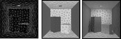
The input of the classic radiosity method consists of a list of patches (triangles, in this example) with their average self-emitted radiosity Bie (left) and reflectivity ρi (middle) given. These data suffice in order to compute the average total radiosities Bi (right), including the effect of light bouncing around. The computed radiosities are converted to display colors for each patch. The resulting, “illuminated,” model can be rendered from any viewpoint, at interactive rates using graphics hardware.
The equations relating Bi with Bie and ρi on all patches are solved, and the resulting radiosities converted to display colors for the surfaces. Since only diffuse illumination is computed, the surface colors are independent from the viewing position. Visualization from an arbitrary viewpoint can be done using graphics hardware, allowing interactive “walks” through an “illuminated” model.
The classic radiosity method is an instance of a larger class of numerical methods called finite element methods [69]. It is a well-known method in heat transfer, and its application to image rendering was introduced in 1984–1985—a few years after the introduction of the classical ray-tracing method [56], [28], [133]. Since these seminal papers appeared, hundreds of follow-up papers have been published, proposing significant improvements and alternatives for computation techniques. Excellent introductory and in-depth overviews of the classic radiosity method can be found in [29, 172]. Here, only a concise derivation of the underlying equations are presented, as well as the traditional way of solving the radiosity equations and a discussion of the main problems of the method.
6.1.2 Mathematical Problem Description
The problem stated above can be described mathematically in three different ways: by the general rendering equation, by a simplification of it for purely diffuse environments, and by a discretized version of the latter.
The General Rendering Equation
As explained in Chapter 2, light transport in a three-dimensional environment is described by the rendering equation. The average radiosity Bi emitted by a surface patch i with area Ai is therefore given by
Bi=1Ai∫Si∫ΩxL(x→Θ) cos(Θ,Nx)dωΘdAx, (6.1)
with (Section 2.6)
L(x→Θ)=Le(x→Θ)+∫Ωxfr(x;Θ′↔Θ)L(x←Θ′)cos(Θ′,Nx)dωΘ′. (6.2)
The Radiosity Integral Equation
On purely diffuse surfaces (Section 2.3.4), self-emitted radiance Le(x) and the BRDF fr(x) do not depend on directions Θ and Θ′. The rendering equation then becomes
L(x)=Le(x)+∫Ωxfr(x)L(x←Θ′) cos(Θ′, Nx)dω′ Θ.
Of course, the incident radiance L(x ← Θ’) still depends on incident direction. It corresponds to the exitant radiance L(y) emitted towards x by the point y visible from x along the direction Θ’ (see Section 2.3.3). As explained in Section 2.6.2, the integral above, over the hemisphere Ωx, can be transformed into an integral over all surfaces S in the scene. The result is an integral equation in which no directions appear anymore:
L(x)=Le(x)+ρ(x)∫SK(x,y)L(y)dAy.
In a diffuse environment (Section 2.3.4), radiosity and radiance are related as B(x) = πL(x) and Be(x) = πLe(x). Multiplication by π of the left- and right-hand sides of the above equation yields the radiosity integral equation:
B(x)=Be(x)+ρ(x)∫SK(x,y)B(y)dAy. (6.3)
The kernel of this integral equation is:
K(x,y)=G(x,y)V(x,y) with G(x,y)=cos(Θxy,Nx)cos(−Θxy,Ny)πr2xy. (6.4)
Θxy is the direction pointing from x to y. r2xy is the square distance between x and y. V(x, y) is the visibility predicate (1 if x and y are mutually visible, 0 otherwise). Equation 6.1 now becomes
Bi=1Ai∫SiL(x)∫Ωxcos(Θ,Nx)dωΘdAx=1Ai∫SiL(x)πdAx=1Ai∫SiB(x)dAx. (6.5)
The Radiosity System of Linear Equations
Often, integral equations like Equation 6.3 are solved by reducing them to an approximate system of linear equations by means of a procedure known as Galerkin discretization [36, 98, 29, 172].
Let’s assume the radiosity B(x) is constant on each patch i, B(x) = Bi’, x ∈ Si. Equation 6.3 can be converted into a linear system as follows:
B(x)=Be(x)+ρ(x)∫SK(x, y)B(y)dAy⇒ 1Ai∫SiB(x)dAx=1Ai∫SiBe(x)dAx +1Ai∫Si∫Sρ(x)K(x, y)B(y)dAy dAx⇔ 1Ai∫SiB(x)dAx=1Ai∫SiBe(x)dAx +∑j1Ai∫Si∫Sjρ(x)K(x, y)B(y)dAydAx⇔ B′i=Bei+∑jB′j1Ai∫Si∫Sjρ(x)K(x, y)dAydAx.
If we now also assume that the reflectivity is constant over each patch, ρ(x) = ρi,x ∈ Si, the following classical radiosity system of equations x) = results:
B′i=Bei+ρi∑jFijB′j. (6.6)
The factors Fij are called patch-to-patch form factors:
Fij=1Ai∫Si∫SjK(x,y)dAydAx. (6.7)
The meaning and properties of these form factors are discussed in Section 6.2. For the moment, the main thing to remember is that they are nontrivial four-dimensional integrals.
Note that the radiosities Bi’ that result after solving the system of linear equations (Equation 6.6) are only an approximation for the average radiosities (Equation 6.5). The true radiosity B(y), which was replaced by B’j in the equations above, is in practice only very rarely piecewise constant! The difference between Bi and Bi’ is, however, rarely visible in practice. For this reason, we will denote both the average radiosity (Equation 6.5) and the radiosity coefficients in Equation 6.6 by Bi in the remainder of this text.
6.1.3 The Classic Radiosity Method
We are now ready to describe the steps of the classic radiosity method. They are:
- Discretization of the input geometry into patches i. For each resulting patch i, a radiosity value (per considered wavelength) Bi will be computed.
- Computation of form factors Fij (Equation 6.7), for every pair of patches i and j.
- Numerical solution of the radiosity system of linear equations (Equation 6.6).
- Display of the solution, including the transformation of the resulting radiosity values Bi (one for each patch and considered wavelength) to display colors. This involves tone mapping and gamma correction (Section 8.2).
In practice, these steps are intertwined: for instance, form factors are only computed when they are needed; intermediate results are displayed during system solution; in adaptive and hierarchical radiosity [30, 64], discretization is performed during system solution, etc.
6.1.4 Problems
Each step of the classic radiosity method is nontrivial, but at first sight, one would expect that Step 3, radiosity system solution, would be the main problem: the size of the linear systems that need to be solved can be very large (one equation per patch; 100,000 patches is quite common). The radiosity system of linear equations is, in practice, very well-behaved, so that simple iterative methods such as Jacobi or Gauss-Seidel iterations converge after relatively few iterations.
The main problems of the radiosity method are related to the first two steps:
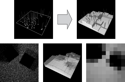
Scene discretization. The patches should be small enough to capture illumination variations such as near shadow boundaries: the radiosity B(x) across each patch needs to be approximately constant. Figure 6.2 shows the image artifacts that may result from an improper discretization. On the other hand, the number of patches shouldn’t be too large, because this would result in exaggerated storage requirements and computation times.
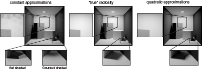
Meshing artifacts in radiosity with constant approximations (left) include undesired shading discontinuities along patch edges. Gouraud shading can be used to blur these discontinuities. Wherever the radiosity varies smoothly, a higher-order approximation of radiosity on each patch results in a more accurate image on the same mesh (a quadratic approximation was used in the right column), but artifacts remain near discontinuities such as shadow boundaries. The middle column shows the “true” radiosity solution (computed with bidirectional path tracing).
Form factor computation. First, even simple objects in a scene may have to be tessellated into thousands of small patches each, on which the radiosity can be assumed to be constant. For that reason, scenes with hundreds of thousands of patches are quite normal. Between each pair of patches, a form factor needs to be computed. The number of form factors can thus be huge (billions) so that the mere storage of form factors in computer memory is a major problem. Second, each form factor requires the solution of a nontrivial, four-dimensional integral (Equation 6.7). The integral will be singular for abutting patches, where the distance rxy in the denominator of Equation 6.4 vanishes. The integrand can also exhibit discontinuities of various degrees due to changing visibility (see Figure 6.3).
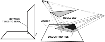
Form factor difficulties: The form factor integral (Equations 6.7 and 6.4) contains the square distance between points in the denominator. This causes a singularity for abutting patches (left). Changing visibility introduces discontinuities of various degrees in the form factor integrand (right). Due to this problem, reliable form factor integration is a difficult task.
Extensive research has been carried out in order to address these problems. Proposed solutions include custom algorithms form factor integration (hemicube algorithm, shaft culling ray-tracing acceleration, etc.), discontinuity meshing, adaptive and hierarchical subdivision, clustering, form factor caching strategies, the use of view importance, and higher-order ra-diosity approximations.
In the algorithms presented in this chapter, the latter problem is addressed by avoiding form factor computation and storage completely. This results in more reliable algorithms (no problems with form factor computational error) that require less storage (no form factors need to be stored). In addition, the presented algorithms are easier to implement and use and result in images of reasonable quality, showing multiple interreflection effects, sometimes much more rapidly than other radiosity algorithms.
The former problem, discretization artifacts, will be addressed using higher-order approximations, and—most importantly—hierarchical refinement and clustering (Section 6.7).
6.2 The Form Factors
The robust and efficient computation of the form factors Fij between each pair of input patches is a major problem with the classic radiosity method. In this section, we will show that the form factors can be viewed as probabilities, and we will present an overview of algorithms for sampling according to form factor probabilities. The fact that form factors are probabilities that can be sampled efficiently leads to algorithms that allow us to solve the radiosity system of equations without the need to ever compute the value of a form factor. These algorithms will be described in Section 6.3 and Section 6.4.
6.2.1 Properties of the Form Factors
Recall that the form factor Fij is given by the following four-dimensional integral (Equation 6.7):
Fij=1Ai∫Si∫SjK(x,y)dAxdAy
with
K(x,y)=cos(Θxy,Nx)cos(−Θxy,Ny)πr2xyV(x,y).
We will need the following properties of the form factors:
- The form factors are all positive or zero in a scene consisting of closed, opaque objects: they cannot be negative because the integrand is positive or zero. They will be equal to zero for a pair of patches i and j that are mutually invisible.
The form factors Fij between a patch i and all other patches j in a scene sum to at most one. If the scene is closed, then
∑jFij=1Ai∫Si∑j∫Sjcos(Θxy, Nx) cos(–Θxy, Ny)πr2xyV(x, y)dAydAx =1Ai∫Si∫Scos(Θxy, Nx) cos(–Θxy, Ny)πr2xyV(x, y)dAydAx =1Ai∫Si1π∫Ωxcos(Θxy, Nx)dωΘxydAx =1Ai∫SiππdAx =1.
If the scene is not closed, the sum of the form factors is less than 1.
The form factors satisfy the following reciprocity relation:
AiFij=Ai1Ai∫Si∫SjK(x, y)dAxdAy =Aj1Aj∫Sj∫SiK(y, x)dAydAx =AjFji.
Any set of positive numbers that sums up to at most one can be regarded as probabilities. For that simple reason, the form factors Fij for a fixed patch i with any other patch j can always be regarded as a set of probabilities.
6.2.2 Interpretation of Form Factors
Let’s recall the radiosity equation (Equation 6.6):
Bi=Bei+ρi∑jFijBj.
This equation states that the radiosity Bi at a patch i is the sum of two contributions. The first contribution consists of the self-emitted radiosity Bei. The second contribution is the fraction of the irradiance (incident radiosity, Section 2.3.1) ∑j FijBj at i that gets reflected. The form factor Fij indicates what fraction of the irradiance on i originates at j.
Recall also that radiosities and fluxes are related as Pi = AiBi and Pei = AiBei (Chapter 2). By multiplying both sides of Equation 6.6 by Ai and using the reciprocity relation (Equation 6.8) for the form factors, the following system of linear equations relating the power Pi emitted by the patches in a scene is obtained:
Bi=Bei+ρi∑jFijBj⇔ AiBi=AiBei+ρi∑jAiFijBj⇔ AiBi=AiBei+ρi∑jAjFjiBj⇔ Pi=Pei+∑jPjFjiρi.
This system of equation states that the power Pi emitted by patch i also consists of two parts: the self-emitted power Pei and the power received and reflected from other patches j. The form factor Fji indicates the fraction of power emitted by j that lands on i, or conversely, Fij indicates the fraction of power emitted by i that lands on j.
Of course, since the form factor is a ratio of positive quantities (radiosity or power), it can’t be negative, giving an intuitive explanation for the first property of form factors above.
The second property (summation to 1) is also easy to see: since there is conservation of radiance, the total amount of power emitted by i and received on other patches j must equal Pi in a closed scene. In a nonclosed scene, some part of the power Pi will disappear into the background, explaining why the sum of the form factors Fij will be less than 1 in that case.
6.2.3 Form Factor Sampling Using Local Lines
The interpretation of a form factor being the fraction of power emitted by a first patch i that lands on a second patch j immediately suggests that form factors can be estimated by means of a very simple and straightforward simulation (see Figure 6.4): Let i be the source of a number Ni of virtual particles that behave like photons originating on a diffuse surface. The number Nij of these particles that land on the second patch j yields an estimate for the form factor: Nij/Ni ≈ Fij.
Indeed, consider a particle originating at a uniformly chosen location x on Si and being shot into a cosine-distributed direction Θ with regard to the surface normal Nx at x. The probability density p(x, Θ) associated with such a particle is
p(x,Θ)=1Ai×cos(Θ, Nx)π.
Note that this PDF is properly normalized:
∫Si∫Ωxp(x,Θ)dAxdωΘ=∫Si1Ai∫Ωxcos(Θ,Nx)πdωΘdAx=1Ai∫SiππdAx=1.
Now, let χj(x, Θ) be a predicate taking value 1 or 0 depending on whether or not the ray shot from x into Θ hits a second patch j. The probability Pij that such a ray lands on a second patch j then is
Pij=∫Si∫Ωxχj(x,Θ)p(x,Θ)dAxdωΘ=∫Si∫Sχj(x,Θ)1Aicos(Θxy,Nx)cos(−Θxy,Ny)πr2xyV(x, y)dAydAx=1Ai∫Si∫Sjcos(Θxy,Nx)cos(−Θxy,Ny)πr2xyV(x, y)dAydAx=Fij.
When shooting Ni such particles from i, the expected number of hits on patch j will be NiFij. As usual in Monte Carlo methods, the more particles shot from i (greater Ni), the better the ratio Nij/Ni will approximate Fij. The variance of this binomial estimator (Section 3.3.1) is Fij(1 — Fij)/Ni. This method of estimating form factors was proposed at the end of the 1980s as a ray-tracing alternative for the hemicube algorithm for form factor computation [171, 167].
As mentioned before, however, we will not need to compute form factors explicitly. The important thing for us is that the probability that a single such particle hits a patch j equals the form factor Fij. In other words, if we are given a patch i, we can select a subsequent patch j among all patches in the scene, with probability equal to the form factor Fij, by shooting a ray from i.
6.2.4 Form Factor Sampling Using Global Lines
The algorithm of the previous section requires us to shoot so-called local lines: lines with an origin and direction selected with regard to a particular patch i in the scene. There exist, however, a number of algorithms for form factor sampling based on uniformly distributed global lines. The origin and direction of global lines is chosen irrespective of any particular surface in the scene, for instance, by connecting uniformly distributed sample points on a bounding sphere for the scene. It can be shown that the probability of finding an intersection of such lines at any given surface location is uniform, regardless of actual scene geometry. The construction and properties of such lines have been studied extensively in the field of integral geometry [155], [160], [161]. Several such sampling algorithms have been proposed for use with radiosity (see, for instance, [160, 142, 128, 161, 189]).
Lines constructed like that will, in general, cross several surfaces in the scene. The intersection points with the intersected surfaces define spans of mutually visible patches along the line (see Figure 6.4). Each such line span corresponds to two local cosine-distributed lines—one in both directions along the line—because the global uniformly distributed lines are uniformly distributed with regard to every patch in the scene. This is unlike local lines, which are uniformly distributed only with regard to the patch on which the origin was sampled.
Form factor sampling: (Left) The fraction of local lines hitting a particular destination patch is an estimate for the form factor between source and destination. Global lines (right) are constructed without reference to any of the patches in the scene. Their intersection points with the surfaces in the scene are, however, also uniformly distributed. The angle between these lines and the normal on each intersected surface is cosine distributed, just like with local lines. The intersection points define spans on each line. Each global line span can be used bidirectionally for form factor computation between the connected patches.
It can be shown that the probability that a global uniform line, generated with the aforementioned algorithms, intersects a given patch i is proportional to the surface area Ai [161]. If N global lines are generated, the number Ni of lines crossing a patch i will be
Ni≈NAiAT. (6.8)
It can also be shown that if Nij is the number of lines that have successive intersections with the surfaces in the scene on patch i and j, then again
NijNi≈Fij.
The main advantage of global lines over local lines is that geometric scene coherence can be exploited in order to generate global lines more efficiently; that is, for the same computation cost, more global line spans can be generated than local lines.
The main limitation of global lines with regard to local lines is that their construction cannot easily be adapted in order to increase or decrease the line density on a given patch. In particular, when used for form factor calculation, it can be shown that the form factor variance is approximately inversely proportional to the area Ai of the source patch i. The variance will be high on small patches.
6.3 Stochastic Relaxation Radiosity
This section and the next one (Section 6.4) cover radiosity algorithms that solve the radiosity system of equations (Equation 6.6) using form factor sampling as discussed in the previous section. We shall see that by doing so, the form factor will appear in the numerator and denominator of the mathematical expressions to be evaluated, so that their numerical value will never be needed. Because of this, the difficult problems of accurately computing form factors and their storage are simply avoided. These algorithms therefore allow much larger models to be rendered with a fraction of the storage cost of other radiosity algorithms. In addition, Monte Carlo radiosity algorithms have a much better time complexity: roughly log-linear in the number of patches rather than quadratic like their deterministic counterparts. In short, they do not only require less storage, but for all but the simplest models, they also finish in less computation time.
There are basically two approaches to solve the radiosity system of linear equations (Equation 6.6) by means of Monte Carlo methods. This section covers the first approach: stochastic relaxation methods; the next section covers the second approach: discrete random walk methods.
The main idea of stochastic relaxation methods is that the radiosity system is solved using an iterative solution method such as Jacobi, Gauss-Seidel, or Southwell iterations [29, 172]. Each iteration of such a relaxation method consists of sums: dot products of a row of the form factor matrix with the radiosity or power vector. When these sums are estimated using a Monte Carlo method, as explained in Section 3.4.2, a stochastic relaxation method results.
6.3.1 The Jacobi Iterative Method for Radiosity
The Basic Idea
The Jacobi iterative method is a method to solve systems of linear equations x = e + Ax using a very simple iteration scheme. Suppose a system with n equations and n unknowns is to be solved. e, x, and any approximation for x are n-dimensional vectors, or points in an n-dimensional Euclidean space. The idea of the Jacobi iterative method is to start with an arbitrary point x(0) in this space. During each iteration, a current point, say x(k), is transformed into a next point x(k+1) by filling in x(k) into the right-hand side of the equations: x(k+1) = e + Ax(k). It can be shown that if A is a contraction, then the sequence of points x(k) will always converge to the same point x, the solution of the system. The point x is also called the fixed point of the iteration scheme. A is a contraction if its matrix norm is strictly less than 1, meaning that repeated application of A will eventually always reduce the distance between transformed points (see Figure 6.5).
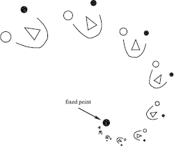
The basic idea of the Jacobi iterative method in two dimensions. The figure in the upper left has been repeatedly scaled down and rotated. As one continues doing so, all points in the plane, including the figure, will be moved towards the dot in the middle. The combination of a rotation and down-scaling transform is a contractive transform. Eventually, all points in the plane are moved closer to each other. The dot in the middle is the fixed point of the transformation, applied repeatedly. In the same way, the right-hand side of the radiosity or power system of equations contains a contractive transformation in n-dimensional space, n being the number of patches. By repeatedly applying this transformation to an arbitrary initial radiosity or power distribution vector, the radiosity problem can be solved.
The coefficient matrix in the radiosity or power system of equations (Equation 6.6 or 6.8) fulfills this requirement. In the context of radiosity, vectors like x and e correspond to a distribution of light power over the surfaces of a scene. L. Neumann [128] suggested viewing the distribution of light power in a scene as a point in such an n-dimensional space and applying the iteration scheme sketched above. The radiosity or power system matrix models a single bounce of light interreflection in the scene. For instance, multiplication with the self-emitted radiosity or power vector results in direct illumination. When applied to direct illumination, one-bounce indirect illumination is obtained. Each Jacobi iteration consists of computing a single bounce of light interreflection, followed by re-adding self-emitted power. The equilibrium illumination distribution in a scene is the fixed point of this process.
Neumann and others suggested numerous statistical techniques for simulating single-bounce light interreflection. The main advantage of these methods over others to be discussed, based on random walks, lies in the fact that simulating a single bounce of light interreflection is an easier problem than simulating any number of bounces at once.
We will now make these statements concrete. First, we show three slightly different ways that repeated single-bounce light interreflection steps can be used in order to solve the radiosity problem. Then, we will focus on the statistical simulation of single-bounce light interreflection.
Regular Gathering of Radiosity
Let’s first apply the above idea to the radiosity system of equations (Equation 6.6). As the starting radiosity distribution Bi(0) = Bei, self-emitted radiosity can be taken. A next approximation Bi(k + 1) is then obtained by filling in the previous approximation B(k) in the right-hand side of Equation 6.6:
B(0)i=BeiB(k+1)i=Bei+ρi∑jFijB(k)j. (6.9)
A hemicube algorithm, for instance [28], allows us to compute all form factors Fij for fixed patch i simultaneously. Doing so, iteration steps according to the above scheme can be interpreted as gathering steps: in each step, the previous radiosity approximations Bj(k) for all patches j are “gathered” in order to obtain a new approximation for the radiosity B(k+1) at i.
Regular Shooting of Power
When applied to the power system, a shooting variant of the above iteration algorithm follows:
P(0)i=PeiP(k+1)i=Pei+∑jP(k)jFjiρi. (6.10)
Using a hemicube-like algorithm again [28], one can compute all form factors Fji for fixed j and variable i at a time. In each step of the resulting algorithm, the power estimate Pi(k + 1) of all patches i, visible from j, will be updated based on Pj(k) : j “shoots” its power towards all other patches i.
Incremental Shooting of Power
Each regular power-shooting iteration above replaces the previous approximation of power P(k) by a new approximation P(k+1). Similar to progressive refinement radiosity [31], it is possible to construct iterations in which unshot power is propagated rather than total power. An approximation for the total power is then obtained as the sum of increments ΔP(k) computed in each iteration step:
ΔP(0)i=PeiΔP(k+1)i=∑jΔP(k)jFjiρi P(k)i=k∑l=0ΔP(l)j.
Discussion
With deterministic summation, there is no difference between the results after complete iterations with the above three iteration schemes. We will see below, however, that they lead to quite different algorithms when the sums are estimated stochastically.
Note that the computation cost of each iteration is quadratic in the number of patches.
6.3.2 Stochastic Jacobi Radiosity
We now discuss what happens if the sums in the above iteration formulae are estimated using a Monte Carlo method. It was explained in Section 3.4.2 that sums can be estimated stochastically by randomly picking terms from the sum according to some probability. The average ratio of the value of the picked terms, over the probability by which they have been picked, yields an unbiased estimate for the sum.
When applied to the above iteration formulae for radiosity, this procedure corresponds to a straightforward simulation of single bounce light interreflection by tracing one-bounce photon paths (see Figure 6.6).
Stochastic Incremental Shooting of Power
Consider the incremental power shooting iterations above. For purely technical reasons, we write the sum ∑jΔP(k)jFjiρi above as a double sum, by introducing Kronecker’s delta function δli = 1 if l = i and 0 if l ≠ i:
ΔP(k+1)i=∑j, lΔP(k)jFjlρlδli. (6.11)
This double sum can be estimated stochastically using any of the form factor sampling algorithms discussed in the previous section:
- Pick terms (pairs of patches) (j, l) in either of the following ways:
- By local line sampling:
Select a “source” patch j with probability pj proportional to its unshot power:
pj=ΔP(k)j/ΔP(k)T with: ΔP(k)T=∑jΔp(k)j.
Select a “destination” patch l with conditional probability pl|j = Fjl by tracing a local line as explained in Section 6.2.3.
The combined probability of picking a pair of patches (j, l) is
Pjl=pjpl/j=ΔP(k)jFjl/ΔP(K)T. (6.12)
By global line sampling (transillumination method [128, 191]), the intersections of each global line (Section 6.2.4) with the surfaces in the scene define spans of mutually visible pairs of points along the line. Each such pair corresponds to a term (j, l) in the sum. The associated probability is
pjl=AjFjl/AT.
- By local line sampling:
Each picked term yields a score equal to the value of that term divided by its probability pjl. The average score is an unbiased estimate for ΔPi(k+1). Estimation with N local lines, for instance, yields
1NN∑s=1ΔP(k)jsFjs,ls ρls δls,iΔP(k)jsFjs,ls/ΔP(k)T=ρiΔP(k)TNiN≈ΔP(k+1)i. (6.13)
Ni=∑Ns=1δls,i is the number of local lines that land on i.
Algorithm 1 Incremental stochastic Jacobi iterative method.
- Initialize total power Pi ← Pei, unshot power ΔPi ← Pei, and received power δPi ← 0 for all patches i and compute total unshot power ΔPT =∑i ΔPi
- Until || ΔPi || ≤ ε or number of steps exceeds maximum, do
- (a) Choose number of samples N.
- (b) Generate a random number ξ ∈ (0,1).
- (c) Initialize Nprev ← 0; q ← 0.
- (d) Iterate over all patches i, for each i, do
- i. qi ← ΔPi/ΔPT.
- ii. q ← q + qi.
- iii. Ni ← ⌊Nq + ξ⌋ – Nprev.
- iv. Do Ni times:
- A. Sample random point x on Si.
- B. Sample cosine-distributed direction Θ at x.
- C. Determine patch j containing the nearest intersection point of the ray originating at x and with direction Θ, with the surfaces of the scene.
- D. Increment δPj←δPj+1NρjΔPT..
- v. Nprev ← Nprev + Ni.
- (e) Iterate over all patches i, increment total power Pi ← Pi + δPi, replace unshot power ΔPi ← δPi, and clear received power δPi ← 0. Compute new total unshot power ΔPT on the fly.
- (f) Display image using Pi.
The procedure above can be used to estimate ΔPi(k+1) for all patches i simultaneously. The same samples (rays or photons) (js, ls) can be used. The difference is only in the scores (Equation 6.13), which basically requires us to count the number of rays hitting each patch. With stratified local line sampling, Algorithm 1 results.
Stochastic Regular Shooting of Power
The sums in regular power-shooting iterations (Equation 6.10) can be estimated using a very similar Monte Carlo method as described above for incremental power shooting. The first stochastic Jacobi radiosity algorithms, proposed by L. and A. Neumann et al. [123], consisted entirely of such iterations. Unlike its deterministic counterpart, the resulting radiosity solutions of each iteration are averaged, rather than having the result of a new iteration replace the previous solution. The main disadvantage of using only regular iterations is that higher-order interreflections appeared in the result only at a slow pace, especially in bright environments. This problem has been called the warming-up or burn-in problem [123, 128, 124, 127].
The warming-up problem can be avoided by first performing a sequence of incremental power-shooting iterations until convergence is obtained, as explained above. This results in a first complete radiosity solution, including higher-order interreflections. Especially when the number of samples N is rather low, this first complete solution will exhibit noisy artifacts. Stochastic regular power-shooting iterations can then be used in order to reduce these artifacts. A regular power-shooting iteration can be viewed as a transformation, transforming a first complete radiosity solution into a new complete one. It can be shown that the output is largely independent of the input. The average of the two radiosity distributions obtained subsequently is to good approximation the same as the result of one iteration with twice the number of samples. Figure 6.6 illustrates this process.
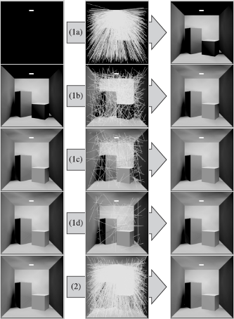
Stochastic Jacobi radiosity in action. (Top left) The initial approximation: self-emitted illumination; (top middle) propagation of self-emitted power by shooting cosine-distributed rays from the light source; (top right) this step results in a first approximation of direct illumination. The next rows (1b)–(1d) illustrate subsequent incremental shooting steps. In each step, the illumination received during the previous step is propagated by shooting cosine-distributed rays. The number of rays is chosen proportional to the amount of power to be propagated so that all rays carry the same amount. After a while, the power to be distributed, and the number of rays, drops below a small threshold. When this happens ((1d), right), a first “complete” radiosity solution is available. This initial solution shows the effect of all relevant higher-order interreflections of light but can be noisy. From that point on, the total power is propagated in so-called regular shooting steps (bottom row). Regular shooting iterations result in new complete solutions, which are, to very good approximation, independent of the input. Noise is reduced by averaging these complete solutions.
Stochastic Regular Gathering of Radiosity
Regular radiosity gathering iterations (Equation 6.9) can be converted into a stochastic variant using the procedure outlined above. The main difference with power-shooting iterations is that now, a new radiosity estimate is obtained as the average score associated with rays that are shot from each patch i, rather than from rays that land on i. Gathering iterations are mainly useful to clean up noisy artifacts from small patches, which have a small chance of being hit by rays in a shooting iteration and therefore exhibit a high variance.
6.3.3 Discussion
Several questions remain to be answered: how shall the number of samples N be chosen; when will the presented algorithms perform well and when will they be suboptimal; and how do they compare? A variance analysis allows us to answer these questions.
The most expensive operation in the algorithms above is ray shooting. The number of rays that needs to be shot in order to compute the radiosities in the scene to given accuracy with given confidence is determined by the variance of the involved estimators.
Incremental Shooting
A detailed analysis of the stochastic incremental shooting algorithm is presented in Appendix C. The results of this analysis can be summarized as follows:
The variance on the resulting radiosity estimates B̃i for each patch i is, to good approximation, given by
V[^Bi]≈PTNρi(Bi−Bei)Ai. (6.14)
In particular, it is inversely proportional to the surface area Ai, meaning that incremental shooting will not be the optimal solution for small patches. Regular gathering does not have this drawback and can be used in order to clean up noisy artifacts on small patches.
The number of samples N in Step 2 (a) of Algorithm 1 shall be chosen proportional to the amount of power ΔPT(k) to be propagated in each iteration, so that rays always carry the same amount of power. A heuristic for the total number of rays in a sequence of iterations until convergence is
N≈9 . maxiρiATAi. (6.15)
In practice, it makes a lot of sense to skip, for instance, the 10% of patches in a scene with the largest ratio ρi/Ai. Note that a rough heuristic for N suffices: a higher accuracy can always be obtained by averaging the result of several independent runs of the algorithm.
- The time complexity of the stochastic Jacobi iterative algorithms for radiosity is roughly log-linear. This is much lower than the quadratic time complexity of deterministic Jacobi iterations.
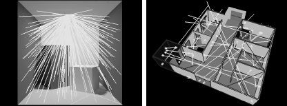
Figure 6.7 illustrates that stochastic relaxation can yield useful images faster than corresponding deterministic relaxation algorithms.
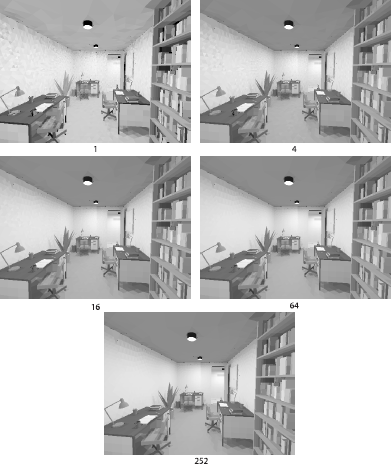
Stochastic relaxation methods can yield useful images much faster than their deterministic counterparts. The environment shown consists of slightly more than 30,000 patches. The top image was obtained with incremental stochastic power-shooting iterations in about 10 seconds on a 2GHz Pentium-4 PC, using about 106 rays. Even if only 1 ray were used for each form factor, 9 · 108 rays would be required with a deterministic method. Noisy artifacts are still visible but are progressively reduced using regular stochastic power-shooting iterations. After about 3 minutes, they are not visible anymore.
This progressive variance reduction is illustrated in the bottom images, shown without Gouraud shading to make noisy artifacts more visible. The shown images have been obtained after 1, 4, 16, 64, and 252 (right-to-left, top-to-bottom) iterations of about 10 seconds each. The model shown is an edited part of the Soda Hall VRML model made available at the University of California at Berkeley.
Regular Shooting
A similar analysis of the variance of regular shooting iterations shows that the variance of a regular shooting iteration, when used with a “complete” radiosity solution as its input, is the same as for a whole sequence of incremental iterations to convergence when the total number of rays being shot is the same. The variance is also given by Equation 6.14. For this reason, the “complete” radiosity results obtained by a sequence of incremental iterations to convergence, and of subsequent regular iterations, are optimally combined by simple averaging.
Regular Gathering
The variance of regular gathering is in practice most often higher than that of shooting, but it does not depend on the patch area. Gathering can therefore be useful in order to “clean” noisy artifacts from small patches, which have a small chance of being hit by shooting rays from elsewhere and can suffer from a large variance with shooting.
Other Stochastic Relaxation Methods for Radiosity
It is possible to design stochastic adaptations of other relaxation methods in the same spirit. Shirley has investigated algorithms that can be viewed as stochastic incremental Gauss-Seidel and Southwell algorithms [167], [169], [168]. Bekaert has studied stochastic adaptations of over-relaxation, Chebyshev’s iterative method, and the conjugate gradient method (suggested by L. Neumann). These relaxation methods have been developed in the hope of reducing the number of iterations to convergence. Since the deterministic iterations have a fixed computation cost, strongly related to the size of a linear system, reducing the number of iterations clearly reduces the total computation cost to convergence. This is, however, not so with the stochastic variants. The computation cost of stochastic relaxation methods is dominated by the number of samples to be taken. The number of samples is only loosely related to the size of the system. In the radiosity case, it turns out that the simple stochastic Jacobi iterations described above are at least as good as other stochastic relaxation methods.
6.4 Discrete Random Walk Methods for Radiosity
In the previous section, a first class of stochastic methods was described for solving the radiosity system of equations (Equation 6.6) or the equivalent power system (Equation 6.8) by means of stochastic variants of well-known iterative solution methods for linear systems, such as the Jacobi iterative method. It was shown that form factor computation and storage is effectively avoided, allowing us to compute radiosity in large models with less computer storage and less computing time than their deterministic counterparts.
This section covers a second class of methods with identical properties. The methods discussed here are based on the concept of a random walk in a so-called discrete state space, explained in Section 6.4.1. Unlike stochastic relaxation methods, random walk methods for linear systems are well covered in Monte Carlo literature [62, 183, 61, 43, 153]. They have been proposed for solving linear systems similar to the radiosity system since the beginning of the 1950s [50, 224]. Their application to radiosity has been proposed in [161, 162].
It turns out that these algorithms are not better than the stochastic Jacobi algorithm of the previous section. We will, however, introduce a number of fundamental concepts that are needed in later sections and chapters, but that are easier to understand first in this context.
6.4.1 Random Walks in a Discrete State Space
Consider the following experiment, involving a set of n urns, labeled i, i = 1, ...,n. One of the urns contains a ball, subject to the following “game of chance”:
- The ball is initially inserted in a randomly chosen urn. The probability that the ball is stored in urn i, i = 1, ...,n, is πi. These probabilities are, of course, properly normalized: ∑ni=1πi=1. They are called source or birth probabilities.
- The ball is randomly moved from one urn to another. The probability pij of moving the ball from urn i to urn j is called the transition probability. The transition probabilities from a fixed urn i need not sum to one. If the ball is in urn i, then the game will be terminated with probability αi=1−∑nj=1pij. αi is called the termination or absorption probability at urn i. The sum of the transition probabilities and the termination probability for any given urn is equal to unity.
- The previous step is repeated until termination is sampled.
Suppose the game is played N times. During the games, a tally is kept of how many times each urn i is “visited” by the ball. It is then interesting to study the expected number of times Ci that the ball will be observed in each urn i. It turns out that
Ci=Nπi+n∑j=1Cjpji.
The first term on the right-hand side of this equation indicates the expected number of times that a ball is initially inserted in urn i. The second term indicates the expected number of times that a ball is moved to urn i from another urn j.
Usually, the urns are called states and the ball is called a particle. The game of chance outlined above is an example of a discrete random walk process. The process is called discrete because the set of states is countable. In Section 6.5, we will encounter random walks in a continuous state space. The expected number of visits Ci per random walk is called the collision density χi. The collision density of a discrete random walk process with source probabilities πi and transition probabilities pij is the solution of a linear system of equations:
χi=πi+n∑j=1χjpji. (6.16)
Note that χi can be larger than unity. For this reason, χi is called the collision density rather than a probability. In summary, we have shown that at least a certain class of linear systems of equations, like the one above, can be solved by simulating random walks and keeping count of how often each state is being visited. The states of the random walk correspond to the unknowns of the system.
6.4.2 Shooting Random Walk Methods for Radiosity
The system of equations in Equation 6.16 is similar to the power system (Equation 6.8):
Pi=Pei+∑jPjFjiρi.
However, the source terms Pei in the power system do not sum to one. Of course, the remedy is very easy: divide both sides of the equations by the total self-emitted power PeT = ∑i Pei:
PiPeT=PeiPeT+∑jPjPeTFjiρi.
This system of equations suggests a discrete random walk process with:
- Birth probabilities πi = Pei/PeT: particles are generated randomly on light sources, with a probability proportional to the self-emitted power of each light source.
- Transition probabilities pij = Fijρj : first, a candidate transition is sampled by tracing, for instance, a local line (Section 6.2.3).1 After candidate transition, the particle is subjected to an acceptance/rejection test with survival probability equal to the reflectivity ρj. If the particle does not survive the test, it is said to be absorbed.
By simulating N random walks in this way, and keeping a count Ci of random walk visits to each patch i, the light power Pi can be estimated as
CiN≈PiPeT. (6.17)
Because the simulated particles originate at the light sources, this random walk method for radiosity is called a shooting random walk method. It is called a survival random walk estimator because particles are only counted if they survive the rejection test (see Figure 6.8).
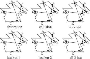
Absorption, collision, and survival random walk estimators differ by when particle hits are counted: only when they are absorbed, only when they survive impact with a surface, or always. The black dots indicate when a particle is counted; a white dot indicates hits at which it is not counted. The score, recorded when a particle is counted, reflects this choice. Absorption, collision, and survival estimation are not the only possibilities. The bottom row shows some alternatives described in the literature.
Usually, particles at the light source are not counted, because they estimate the self-emitted light distribution, which is known. We call this source term estimation suppression.
Collision Estimation
Transition sampling as described above is suboptimal. Candidate transition sampling involves an expensive ray-shooting operation. If the candidate transition is not accepted, this expensive operation has been performed in vain. This will often be the case if a dark surface is hit. It will always be more efficient to count the particles visiting a patch, whether they survive or not. The estimates (Equation 6.17) then, of course, need to be reduced in order to compensate for the fact that too many particles are counted. The resulting collision random walk estimates are
ρiC′iN≈PiPeT. (6.18)
Ci′ denotes the total number of particles hitting patch i. The expected number of particles that survive on i is ρiCi′ ≈ Ci.
Absorption Estimation
A third, related, random walk estimator only counts particles if they are absorbed. The resulting absorption random walks estimates are
ρi1−ρiC″iN≈PiPeT. (6.19)
Ci″ denotes the number of particles that are absorbed on i. It fulfills Ci’ = Ci + Ci″. The expected number of particles being absorbed on i is (1 – ρi)C’i ≈ Ci″. The collision estimator is usually, but not always, more efficient than the absorption estimator. A detailed comparison can be made by computing the variance of the random walk methods (Section 6.4.4).
6.4.3 Adjoint Systems, Importance or Potential, and Gathering Random Walk Methods for Radiosity
The estimators above are called shooting estimators, because they simulate the trajectory of imaginary particles that originate at a light source. The particles are counted whenever they hit a patch of which we want to estimate the light power. Alternatively, it is also possible to estimate the radiosity on a given patch i, by means of particles that originate at i and that are counted when they hit a light source. Such gathering random walk estimators can be derived in a brute force manner, analogous to the development of the path-tracing algorithm in Chapter 5. There is, however, also a more elegant, although slightly more abstract, interpretation of gathering random walk estimators: a gathering random walk estimator corresponds to a shooting random walk estimator for solving an adjoint system of equations.
Adjoint systems of equations. Consider a linear system of equations Cx = e, where C is the coefficient matrix of the system, with elements cij; e is the source vector; and x is the vector of unknowns. A well-known result from algebra states that each scalar product 〈x, w〉=∑ni=1xiwi of the solution x of the linear system, with an arbitrary weight vector w, can also be obtained as a scalar product 〈e, y〉 of the source term e with the solution of the adjoint system of linear equations C⊤y = w:
〈w, x〉=〈C⊤y, x〉=〈y, Cx〉=〈y, e〉.
C⊤ denotes the transpose of the matrix C: if C = {cij}, then C⊤ = {cji}. The second equality in the derivation above is a fundamental property of scalar products, which is extremely easy to verify yourself.
Adjoints of the radiosity system, and the concept of importance or potential. Adjoint systems corresponding to the radiosity system of equations (Equation 6.6) look like:
Yi=Wi+∑jYjρjFji. (6.20)
These adjoint systems and the statement above can be interpreted as follows (see Figure 6.9): Consider the power Pk emitted by a patch k. Pk can be written as a scalar product Pk = AkBk = 〈B, W〉 with Wi = Aiδik: all components of the direct importance vector W are 0, except the kth component, which is equal to Wk = Ak. The statement above implies that Pk can also be obtained as Pk = 〈Y,E〉 =∑iYiBei, which is a weighted sum of the self-emitted radiosities at the light sources in the scene. The solution Y of the adjoint system (Equation 6.20) indicates to what extent each light source contributes to the radiosity at k. Y is called the importance or potential in the literature [181], [140], [25]; see also Section 2.7.
Duality between gathering and shooting in radiosity. The light flux emitted by the patch shown in bright in the top right image can be obtained in two ways: 1) as the scalar product of radiosity B (top left) and the response or measurement function W (top right), and 2) as the scalar product of the self-emitted radiosity E (bottom left) with importance Y (bottom right).
Gathering random walk estimators for radiosity. The adjoints (Equation 6.20) of the radiosity system also have the indices of the form factors in the right order, so they can be solved using a random walk simulation with transitions sampled with local or global lines. The particles are now, however, shot from the patch of interest (πi = δki), instead of from the light sources. The transition probabilities are pji = ρjFji: First, an absorption/survival test is performed. If the particle survives, it is propagated to a new patch, with probabilities corresponding to the form factors. A nonzero contribution to the radiosity of patch k results whenever the imaginary particle hits a light source. Its physical interpretation is that of gathering.
The gathering random walk estimator described here is a collision estimator. It is possible to construct a survival or absorption gathering estimator as well. A survival gathering random walk estimator will only count particles that survive on a hit light source, for instance.
6.4.4 Discussion
Discrete random walk estimators for radiosity thus can be classified according to the following criteria:
- Whether they are shooting or gathering.
- According to where they generate a contribution: at absorption, survival, at every collision.
In order to make statements about how these variants compare with each other and with the stochastic Jacobi method discussed in the previous section, the variance of these methods needs to be computed. Except for the variance of the absorption estimators, which are simple hit-or-miss estimators, the calculation of random walk variances is fairly complicated and lengthy. The results are summarized in Table 6.1 and Table 6.2. The derivation of these results can be found in [161], [162], [15].
Score and variance of discrete shooting random walk estimators for radiosity.
estimatior |
score ˜s(j0,...,jτ) |
variance V[˜s] |
|---|---|---|
absorption |
ρkAkPeT1−ρkδjτk |
ρkAkPeT1−ρkbk−b2k |
collision |
ρkAkPeT∑τt=1δjtk |
ρkAkPeT(1+2ςk)bk−b2k |
survival |
1AkPeT∑τ−1t=1δjtk |
1AkPeT(1+2ςk)bk−b2k |
Score and variance of discrete gathering random walk estimators for radiosity.
estimatior |
score ˜s(j0 = k,...,jτ) |
variance V[˜sk] |
|---|---|---|
absorption |
ρkBejτ1−ρjτ |
ρk ∑sBes1−ρsbks−b2k |
collision |
ρk ∑τt=1Bejt |
ρk ∑s(Bes+2bs)bks−b2k |
survival |
ρk ∑τ−1t=1Bejtρjt |
ρk ∑sBes+2bsρsbks−b2k |
In Table 6.1, j0 is the patch at which a random walk originates. It is a patch on a light source in the scene, chosen with probability proportional to its self-emitted power. j1,..., jτ are the patches subsequently visited by the random walk. Transitions are sampled by first doing a survival/absorption test, with survival probability equal to the reflectivity. After survival, the next visited patch is selected with probability equal to the form factor, by tracing local or global lines. τ is the length of the random walk: The random walk is absorbed after hitting the patch jτ. The expectation of all these estimators is equal to the non-self-emitted radiosity bk = Bk — Bek at a patch k (source term estimation is suppressed). ζk is the recurrent radiosity at k: If k is the only source of radiosity, with unit strength, the total radiosity on k would be larger than 1, say Ik, because other patches in the scene reflect part of the light emitted by k back to k. The recurrent radiosity then would be ζk = Ik – 1. The recurrent radiosity also indicates the probability that a random walk visiting a patch k will return to k. Usually, this probability is very small, and the terms containing ζk can be ignored.
Table 6.2 shows the score and variance of discrete gathering random walks. The expectation is bk = Bk – Bek, as well, but this time k refers to the patch on which the random walk originates: k = j0. Transitions are sampled exactly as for shooting random walks. bks is the radiosity at k due to the light source s, received directly or via interreflections from other patches: bk = ∑s bks.
Shooting versus Gathering
The variance expressions in Table 6.1 and Table 6.2 allow us to make a detailed theoretical comparison of discrete shooting and gathering random walks. The shooting estimators have lower variance, except on small patches, which have low probability of being hit by rays shot from light sources. Unlike shooting estimators, the variance of gathering estimators does not depend on the patch area Ak. For sufficiently small patches, gathering will be more efficient. Gathering could, like in the case of stochastic relaxation methods, be used in order to “clean” noisy artifacts on small patches after shooting.
Absorption, Survival, or Collision?
The variance results in Table 6.1 and Table 6.2 also indicate that the survival estimators are always worse than the corresponding collision estimators, because the reflectivity ρk (shooting) or ρs (gathering) is always smaller than 1.
As a rule, the collision estimators also have lower variance than the absorption estimators:
- Shooting estimators: the recurrent radiosity ζk is, in general, negligible and 1 – ρk < 1.
- Gathering estimators: as a rule, self-emitted radiosity Bes of a light source is much larger than the non-self-emitted radiosity bs, and again, 1 – ρs < 1.
These results hold when transitions are sampled according to the form factors. When the transition probabilities are modulated, for instance, to shoot more rays into important directions (Section 6.6.1), an absorption estimation can sometimes be better than a collision estimator. In particular, it can be shown that a collision estimator can never be perfect, because random walks can contribute a variable number of scores. An absorption estimator always yields a single score, so it does not suffer from this source of variance. For this reason, absorption estimators can be made perfect, at least in theory.
Discrete Collision Shooting Random Walks versus Stochastic Jacobi Relaxation
According to Table 6.1, the variance of NRW discrete collision shooting random walks is approximately
VRWNRW≈1NRWρkAkPeT(Bk−Bek).
The variance of incremental power shooting (Equation 6.14) with NSR rays is approximately
VSRNSR≈1NSRρkAkPT(Bk−Bek).
It can be shown that NRW random walks result on the average in NRWPT/PeT rays to be shot. Filling in NSR = NRWPt/PeT in the expression above thus indicates that for the same number of rays, discrete collision shooting random walks and incremental power-shooting Jacobi iterations are approximately equally efficient. This observation has been confirmed in experiments [11].
This rather unexpected result can be understood as follows. Both algorithms have an intuitive interpretation in the sense of particles being shot from patches. The particles have a uniform starting position on the patches, and they have cosine-distributed directions with regard to the normal on the patches. The number of particles shot from each patch is proportional to the power propagated from the patch. Since the two methods compute the same result, the same number of particles will be shot from each of the patches. If the same random numbers are also used to shoot particles from each patch, the particles themselves can also be expected to be the same. The main difference is the order in which the particles are shot: they are shot in “breadth-first” order in stochastic relaxation and in “depth-first” order with random walks (see Figure 6.10). For the variance, this makes no difference.
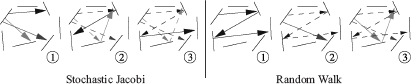
This figure illustrates the difference in order in which particles are shot in stochastic Jacobi iterations (“breadth-first” order) and in collision shooting random walk radiosity (“depth-first” order). Eventually, the shot particles are very similar.
There are, however, other, more subtle differences between the algorithms, in particular in the survival sampling: In the random walk algorithm, the decision whether a particle will survive on a patch or not is made independently for all particles. In stochastic relaxation radiosity, the decision is made once for a group of particles that landed on a patch during a previous iteration step. For instance, if 10 particles land on a patch with reflectivity 0.45, in the random walk method, any number of particles, ranging from 0 to 10, might survive on the patch. In the stochastic relaxation algorithm, the number of surviving particles will be 4 or 5. In both cases, the average will be 4.5. Experiments with very simple scenes, such as an empty cube, where recurrent radiosity ζk is important, do reveal a different performance [11].
The conclusion that stochastic Jacobi iterations and random walks are equally efficient is also no longer true when higher-order approximations are used, or with low-discrepancy sampling, or in combination with variance reduction techniques. Many variance-reduction techniques and low-discrepancy samplings are easier to implement and appear more effective for stochastic relaxation than with random walks (see Section 6.6).
6.5 Photon Density Estimation Methods
The algorithms discussed in Section 6.3 and Section 6.4 solved the radiosity system of linear equations (Equation 6.6) stochastically. By sampling according to the form factors, the numerical value for the form factors was never needed. In this section, we will discuss a number of random walk methods that are highly related to those of Section 6.4, but that solve the radiosity integral equation (Equation 6.3), or the general rendering equation (Equation 6.2), rather than the radiosity system of equations. Indeed, just like discrete random walks are used to solve linear systems, random walks in a continuous state space can be used to solve integral equations like the radiosity or rendering integral equation. They are, therefore, sometimes also called continuous random walk radiosity methods.
The random walks that are introduced in this section are nothing but simulated trajectories of photons emitted by light sources and bouncing throughout a scene, as dictated by the laws of light emission and scattering described in Chapter 2. The surface hit points of these photons are recorded in a data structure, for later use. An essential property of such particle hit points is that their density at any given location (the number of hits per unit of area) is proportional to the radiosity at that location (Section 6.5.1). This density can be estimated at any surface location where this needs to be done, by means of density estimation methods known from statistics [175]. The basic density estimation methods that have been used for global illumination are covered in Section 6.5.2, Section 6.5.3, Section 6.5.4, Section 6.5.5. In addition, the instant radiosity algorithm by Keller [91] fits in this class (Section 6.5.6).
The main benefit of this approach is that nondiffuse light emission and scattering can be taken into account to a certain extent. Just like the methods of the previous sections, the methods described here do not allow us to solve the rendering equation exactly at every surface point. Still, some world-space representation of the illumination on the surfaces in the scene needs to be chosen, with corresponding approximation errors like blurred shadow boundaries or light leaks. However, photon density estimation methods open the way to more sophisticated and pleasing representations of the illumination than the average radiosity on surface patches. For this reason, they have gained considerable importance and attention in the last years. In the photon-mapping method, for instance, [83], the representation of illumination is independent of scene geometry. This allows us to use nonpolygonized geometry representations, procedural geometry such as fractals, and object instantiation in a straightforward manner.
6.5.1 Photon Transport Simulation and Radiosity
Photon trajectory simulation, according to the laws of physics as outlined in Chapter 2, is called analog photon trajectory simulation. We start by explaining how analog photon trajectory simulation works and how it can be used for computing radiosity. Figure 6.11 illustrates this process.
We start out (1a) by selecting an initial particle location x0 on a light source. We do that with a (properly normalized) probability proportional to the self-emitted radiosity:
S(x0)=Be(x0)PeT. (6.21)
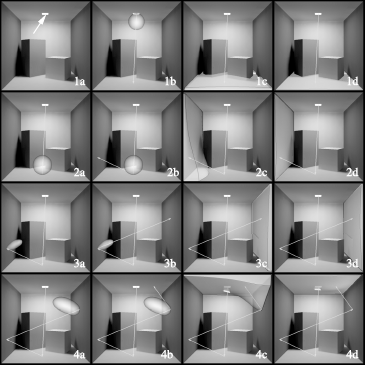
Analog photon transport simulation, from the selection of an initial particle location to absorption.
x0 is the starting point for a random walk. S(x0) is called the birth or source density.
Next, an initial particle direction Θ0 is selected using the directional light emission distribution of the light source at x0, times the outgoing cosine. For a diffuse light source (1b),
T(Θ0|x0)=cos (Θ0,Nx0)π.
Consider now a ray shot from the sampled location x0 into the selected direction Θ0. The density of hit points x1 of such rays with object surfaces depends on surface orientation, distance, and visibility with regard to x0:
T(x1|x0,Θ0)=cos (−Θ0,Nx1)r2x0x1V(x0,x1).
The transparent surface in (1c) shows this density on the bottom surface of the shown model. In (1d), the density of incoming hits is shown, taking into account these geometric factors as well as the (diffuse) light emission characteristics at x0:
Tin(x1|x0)=T(Θ0|x0)T(x1|x0,Θ0) =cos (Θ0,Nx0)cos (−Θ0,Nx1)πr2x0x1 V(x0,x1)=K(x0,x1).
Next, (2a), a survival test is carried out at the obtained surface hit point x1: A random decision is made whether or not to sample absorption (and path termination) or reflection. We take the probability σ(x1) of sampling reflection equal to the albedo ρ(x1, – Θ0), the fraction of power coming in from x0 that gets reflected at x1. For a diffuse surface, the albedo is the same as the reflectivity ρ (x1). The full transition density from x0 to x1 is thus
T(x1|x0)=Tin(x1|x0)σ(x1)=K(x0,x1)ρ(x1). (6.22)
If survival is sampled, a reflected particle direction is chosen according to the BRDF times the outgoing cosine. For a diffuse surface, again only the outgoing cosine remains (2b).
Subsequent transitions are sampled in the same way, by shooting a ray, performing a survival test, and sampling reflection if the particle is not absorbed. Image (2c) shows the influence of surface orientation, distance, and visibility on the left surface of the scene with regard to x1. (2d) shows the combined effect of the cosine distribution at x1 and the former. The third and fourth rows of Figure 6.11 illustrate the process twice more, this time for nondiffuse reflection.
Now, consider the expected number χ(x) of particle hits resulting from such a simulation, per unit of area near a surface location x. This particle hit density consists of two contributions: the density of particles being born near x, as given by S(x), and the density of particles visiting x after visiting some other surface location y. The density of particles coming from elsewhere depends on the density χ(y) elsewhere and the transition density T(x|y) to x:
χ(x)=S(x)+∫sχ(y)T(x|y)dAy.
For a diffuse environment, the birth and transition density are given by Equation 6.21 and Equation 6.22:
In other words, the number of particle hits per unit area expected near a surface location x is proportional to the radiosity B(x). We have derived this result for diffuse environments here, but also with nondiffuse light emission and scattering, the particle hit density after analog simulation will be proportional to the radiosity. This is illustrated in Figure 6.12. This is, of course, not a surprise: it is our mental model of how nature works, and which we simulate in a straightforward manner on the computer.
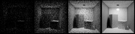
The density of particle hits after a photon transport simulation according to the physics of light emission and scattering, is proportional to the radiosity function. These images show the particle hits of 1,000, 10,000, 100,000, and 1,000,000 paths, respectively.
The problem of computing radiosity has thus been reduced to the problem of estimating particle hit densities: to estimating the number of particle hits per unit area at a given surface location. The problem of estimating a density like that, given nothing more than a set of sample point locations, has been studied intensively in statistics [175]. The next sections cover the main density estimation methods that have been applied in the context of rendering: histogram methods, orthogonal series estimation, kernel methods, and nearest neighbor methods.
An alternative, equivalent point of view is to regard the problem at hand as a Monte Carlo integration problem: we want to compute integrals of the unknown radiosity function B(x) with a given measurement, or response, function M(x) (see also Section 2.8):
The radiosity B(x), and thus the integrand, cannot be evaluated a priori, but since analog simulation yields surface points xs with density χ(xs) = B(xs)/PeT, M can be estimated as
Basically, all we have to do is simulate a number of photon trajectories and accumulate the value of measurement function M(xs) at the photon surface hit points xs.2 The measurement functions corresponding to histogram methods, orthogonal series estimation, and kernel methods are described below.
Note that the procedure explained here corresponds closely with the survival estimator in Section 6.4.1: Particles are only taken into account after surviving impact on a surface. Just like before, absorption and collision estimators can be defined, and source term estimation can be suppressed. In practice, collision estimation, that is, counting all particles that land on a surface, is preferred. Like before, this “over-counting” shall be compensated by multiplying all resulting expressions by the reflectivity.
6.5.2 Histogram Methods
The easiest, and probably most often used, way of estimating density functions is by subdividing the domain of the samples into bins—surface patches in our case—and to count the number of samples Ni in each bin (Figure 6.13). The ratio Ni/Ai yields an approximation for the particle density in each bin.
The histogram method, illustrated for the particle hits on the bottom side of the cube shown in Figure 6.12.
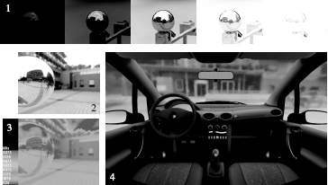
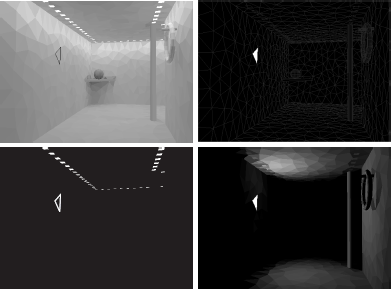
Image 4 shows the result of a real-world lighting simulation in a car model. A histogram method (Section 6.5.2) was used. Real-world lighting was captured by photographing a mirror sphere at various shutter speeds (1), and combining these images into a single high dynamic range environment map. Image 2 shows a mirror sphere, ray traced using this environment map. Image 3 shows the color-coded illumination levels from Image 2, which vary between 200 and 30,000 nits. The histogram method, like most other stochastic radiosity methods, handles arbitrary light sources such as this high dynamic range environment map with ease. (See Plate II.)
![Figure showing these images have been rendered using a histogram method [206] taking into account measured BRDFs. Specular effects have been added by ray tracing in a second pass. (Images courtesy of F. Drago and K. Myszkowski, Max-Planck-Institute for Informatics, Saarbrücken, Germany.) (See Plate III.)](http://imgdetail.ebookreading.net/software_development/6/9781439864951/9781439864951__advanced-global-illumination__9781439864951__image__190x002.png)
These images have been rendered using a histogram method [206] taking into account measured BRDFs. Specular effects have been added by ray tracing in a second pass. (Images courtesy of F. Drago and K. Myszkowski, Max-Planck-Institute for Informatics, Saarbrücken, Germany.) (See Plate III.)
An alternative explanation is as follows: Recall that the average radiosity on a patch i is by definition given by the following integral of B(x):
A random walk constructed as outlined is a technique to sample points x with density χ(x) = B(x)/PeT. With N random walks, Bi can be estimated as
where Ni is the number of visits to the patch i. The measurement functions Mhist(x) of histogram methods are the so-called characteristic functions of the surface patches: functions taking value 1 for points on the surface patch, and 0 for other points.
Histogram methods for radiosity computations have been proposed in [5], [70], [138] and by others later on. This form of density estimation is very popular because of its simplicity.
6.5.3 Orthogonal Series Estimation
Histogram methods yield a single average radiosity value for each surface patch. It is possible to obtain linear, quadratic, cubic, or other higher-order approximations for the radiosity function B(x), too. The problem of computing such higher-order approximations comes down to computing the coefficients Bi,α in the following decomposition of B(x):
The functions ψi, α(x) are called basis functions. The sum is over all basis functions defined on patch i. A constant approximation is obtained when using just one basis function ψi(x) per patch, which is 1 on the patch and 0 outside. In that case, we will again obtain the histogram method of the previous section. Figure 6.16 illustrates higher-order basis functions that can be used on quadrilaterals. The idea is to approximate B(x) as a linear combination of such functions.
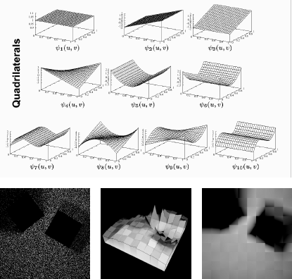
The top image shows a set of orthogonal functions, usable for orthogonal series estimation on quadrilaterals. The bottom image shows a linear approximation for the density of the particle hits on the bottom side of the cube shown in Figure 6.12.
The coefficients Bi, α can be obtained as scalar products with so-called dual basis functions ψ̃i, α:
Each dual basis function ψ̃i, α is the unique linear combination of the original basis functions ψ̃i, β that fulfills the relations (fixed α, variable β)
In the case of a constant approximation, the dual basis function is ψ̃i (x) = 1/Ai if x ∈ Si and 0 elsewhere.
With N photon trajectories, Equation 6.24 can be estimated as
The sum is over all points xs visited by the random walks. The measurement functions of orthogonal series estimation are the dual basis functions ψ̃i, α.
Radiosity computation by orthogonal series estimation, as such methods are called, has been proposed by Bouatouch et al. [18] and Feda [44].
The main advantage of orthogonal series estimation over the histogram method is that a smoother approximation of radiosity is possible on a fixed mesh. Its main disadvantage is the cost. One can show [44, 13] that the cost of computing a higher-order approximation with K basis functions to fixed statistical error is about K times the cost of computing a constant approximation. The increase in computation time for higher-order approximations is larger than in deterministic methods [69, 228], but the resulting algorithms are significantly easier to implement, still require no form factor storage, and are much less sensitive to computational errors (see Figure 6.17).
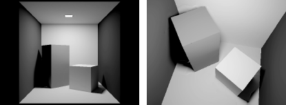
Two images generated from the same converged cubic approximation solution. Once the solution has been obtained, a new image for a new viewpoint can be generated in fractions of a second. These images illustrate that orthogonal series estimation (as well as stochastic relaxation methods for higher-order approximations) can result in very high image quality in regions where illumination varies smoothly. In the neighborhood of discontinuities, however, image artifacts may remain. Discontinuity meshing would eliminate these artifacts.
6.5.4 Kernel Methods
The radiosity B(z) at a point z could also be written as an integral involving a Dirac impulse function:
Estimating the latter integral with random walks wouldn’t work, because the Dirac pulse function is zero everywhere, except when its argument is zero. The chance of finding a particle hitting exactly the point z is zero in theory3 Even if we could find a particle hitting exactly at z, the value of the Dirac pulse is not determinate. It can’t be finite because the Dirac function is zero everywhere except at one point and its integral is equal to 1. An approximation for the radiosity at z can, however, be obtained by using a different, normalized density kernel or footprint function f(x, z) with nonzero width centered around z:
Usually, a symmetric kernel is chosen, which depends only on the distance between x and z: F(x,z) = F(z,x) = F(rxz). Examples include a cylindrical kernel (F(r) = 1/2πR if r < R and 0 otherwise) or a Gaussian bell.
With N photon trajectories, the integral in Equation 6.25 can be estimated as
The sum is again over all points xs visited by the random walks. The measurement functions this time are the kernels F(x,z), centered at the query locations z.
For symmetric kernels, one can also interpret this result as follows: A kernel Fs(z) = F(xs, z) is placed at every particle hit point xs. The radiosity estimate at a surface point z is then obtained by summing the value of these kernels at z.
This form of kernel density estimation has been used by Chen [24], Collins [32], and Shirley and Walter et al. [166, 210].
The main advantage of kernel methods is that they allow a representation of illumination that is not necessarily mesh-based, or that allows a suitable mesh to be constructed a posteriori. This allows us to get rid of edge discontinuities (see Figure 6.2). On the other hand, the choice of the kernel bandwidth is a difficult problem, and a lot of effort is required in order to avoid underestimation at surface edges, called boundary bias (see Figure 6.18). The cost of kernel evaluation can be considerable too, for instance, for a Gaussian kernel.
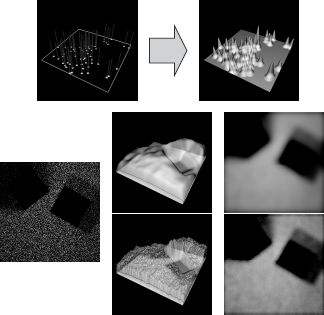
Kernel methods can be viewed as follows: A normalized kernel function is placed centered at each particle hit point. Radiosity is estimated by summing these kernels. The bottom rows of this figure show the result with a cylindrical kernel (middle row) and a Gaussian kernel (bottom row). The kernels have the same bandwidth. A Gaussian kernel results in a smoother result but at a higher computation cost than a cylindrical kernel. Note that the resulting radiosity estimates at the edges are only half of what they should be. This effect, due to the fact that the area on which particles are found around a query location is constrained (no particles beyond the edge), is called boundary bias.
![Figure showing images obtained with the kernel density estimation method from [210]. Kernel density estimation allows for a posteriori meshing: A mesh capturing the illumination variations in the scene accurately is constructed after particle tracing and density estimation. The resulting mesh can be rendered in real time using graphics hardware.](http://imgdetail.ebookreading.net/software_development/6/9781439864951/9781439864951__advanced-global-illumination__9781439864951__image__195x002.png)
Images obtained with the kernel density estimation method from [210]. Kernel density estimation allows for a posteriori meshing: A mesh capturing the illumination variations in the scene accurately is constructed after particle tracing and density estimation. The resulting mesh can be rendered in real time using graphics hardware.
(Images courtesy of B. Walter, Ph. Hubbard, P. Shirley, and D. Greenberg, Cornell Program of Computer Graphics.) (See Plate IV.)
6.5.5 Nearest Neighbor Methods
The photon-mapping algorithm by Jensen et al. [81] and Keller’s instant radiosity algorithm [91] are based on a similar principle.
Photon mapping uses a technique called nearest neighbor estimation. Nearest neighbor estimation can be understood as follows (see Figure 6.20): Rather than fixing a certain area A and counting the number of particles N on that area like in the histogram method, one fixes a number of particles N and looks for an area that contains this number of particles. If N particles can be found on a small area, the density (N/A) will be high. If they are only found on a large area, the density will be low. The main advantage of nearest neighbor estimation is that one can entirely get rid of surface meshes. All one needs to store is the set of particle hit-point locations. Photon mapping will be explained in detail in Section 7.6.
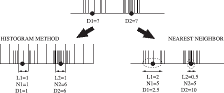
Two ways to estimate the density of samples D1 and D2 near the indicated locations (top row): 1) histogram methods (bottom left) first subdivide the domain into bins (the size of the bins here is L = 1) and count the number of samples N1 and N2 in the bins where density needs to be estimated; and 2) nearest neighbor estimation methods (bottom right) fix a number of samples N (here: N = 5) and find regions at the query locations that contain this number of samples (size L1 and L2). In both cases, density is estimated as the number of samples N over the size L of the considered regions. In the limit for a large number of samples and small bins, these methods will yield identical results.
The measurement functions corresponding to nearest neighbor estimation are more complex than for the previous density estimation methods. They depend on the whole set of sample locations and therefore can only be evaluated a posteriori [175, Chapter 1].
6.5.6 Instant Radiosity
Instant radiosity [91] is based on the following observation: The right-hand side of the radiosity integral equation (Equation 6.3) is also an integral containing the radiosity function
Here too, this integral can be estimated by tracing a number of photon trajectories. This results in estimates for B(z) of the following form:
The sum in the right-hand side can be interpreted as the direct illumination at z due to point light sources with strength PeT/N placed at every photon hit point xs. Instant radiosity will be explained in more detail in Section 7.7.
6.5.7 Discussion
We now discuss gathering variants and compare the algorithms with each other and with discrete random walk methods for radiosity.
Continuous Gathering Random Walks
The algorithms explained in this section are shooting algorithms. Just like with discrete random walk methods (Section 6.4.3), gathering variants can be obtained by introducing adjoints of an integral equation. Adjoints of the radiosity integral equation, for instance, look like
Their interpretation is exactly the same as explained in Section 6.4.3. Continuous gathering random walks are the basis of path-tracing algorithms discussed in Chapter 5. They have received little attention for the computation of world-space illumination representations. They may, however, help to “clean up” noisy artifacts on small patches in the histogram method, or when orthogonal series estimation is used. They might also be valuable in the context of bidirectional algorithms for object-space illumination computation, complementing shooting random walks.
Variance
A detailed comparison of various continuous random walk estimators among each other, or continuous versus discrete random walks, requires that the variance of the continuous random walk estimators be calculated. The calculation of continuous random walk variances can be done in exactly the same way as for a discrete random walk. A compact derivation, based on Green’s function for the radiosity integral equation, can be found in [11]. The result for a continuous collision shooting random walk method with source term estimation suppression and using measurement function M(x) is
In this equation, ζ(x) = I(x) – M(x), with I(x) the solution of the adjoint integral equation (Equation 6.26) with source term M(x). Most often, ζ(x) is much smaller than 1, so it can be ignored. The expected value is bM = ∫ M(x)b(x)dAx with b(x) = B(x) – Be(x), the non-self-emitted radiosity. By filling in the appropriate response functions M(x), the variance can be computed for any of the aforementioned density estimation methods.
Bias
All density estimation algorithms described here compute a kind of convolution of the radiosity function:
The approximations are visible in the images in the form of artifacts such as blurred shadow boundaries, edge discontinuities and light or shadow leaks, and boundary bias artifacts. For this reason, the density estimates are often not directly visualized, but a final gathering step is performed in order to avoid artifacts. Final gathering, and other hybrid methods, are the topic of Chapter 7.
It can be shown that all density estimation methods discussed here share a similar bias versus variance trade-off (see Figure 6.21 and Figure 6.22): A response function with a large support, for instance, a histogram method on large patches, or a kernel method with wide kernels, will yield a lower variance. On the down side, however, a large support in general also means worse blurring of the radiosity function. The converse is true as well: narrow response functions reduce blurring and therefore result in, for instance, sharper shadow boundaries, but at the cost of a higher variance.
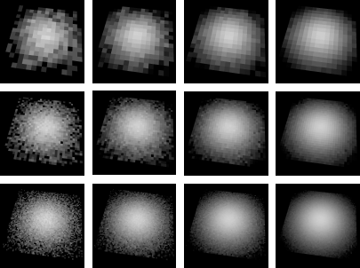
Variance versus bias trade-off of density estimation algorithms: The same scene is shown in all images, with increasingly fine discretization top-to-bottom and increasing number of samples left-to-right. The number of patches is 256 in the top row, 1024 in the middle row, and 4096 in the bottom row. The number of samples has been taken proportional to the number of patches: 10 times the number of patches (left), 40 times, 160 times, and 640 times (right). These images illustrate that the variance of the histogram method is inversely proportional to the patch area: images in the same column have the same variance. All other photon density estimation algorithms exhibit a similar variance versus bias trade-off as well.
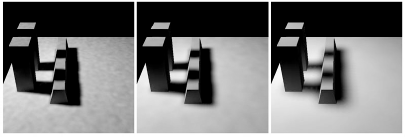
Variance versus bias trade-off in a kernel density estimation method: The number of particles is kept the same. The kernel bandwidth has been increased from left to right. A large bandwidth (right) yields low noise but blurred radiosity results.
(Image courtesy of B. Walter, Ph. Hubbard, P. Shirley, and D. Greenberg, Cornell Program of Computer Graphics).
Continuous versus Discrete Random Walks
Continuous random walks with the histogram method and discrete random walks solve different problems. Continuous random walks with the histogram method estimate the area average of the continuous radiosity function B(x) over a patch. Discrete random walks estimate the solution of a linear system of equations. The difference in practice, however, is only rarely noticeable: both methods can suffer from light leaks, for instance, but leaked light will illuminate other surfaces with a discrete random walk, whereas it won’t with a continuous random walk method.
The algorithmic difference is quite small, also, with a continuous random walk; a particle is always reflected from its point of incidence on a patch. In a discrete random walk, a particle is reflected from a uniformly chosen different location on the patch on which it lands (see Figure 6.23).
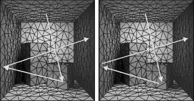
Continuous (left) versus discrete (right) random walks differ slightly in the way particles are reflected: Particles reflect off their point of incidence in continuous random walks. In discrete random walks, they emerge from a uniformly chosen new location on the patch they hit.
Experiments in which a continuous and discrete collision shooting random walk have been compared indicate that there is also no significant difference in variance. This can be explained by comparing Equation 6.27 to the histogram method with the variance of the discrete collision shooting random walk in Table 6.1 on page 181. The response function for the histogram method is M(x) = χk(x)/Ak with χk(x), the characteristic function of a patch k.
Low-discrepancy sampling, however, appears to be significantly more effective with the discrete random walk than with the continuous random walk [15].
6.5.8 Stochastic Iteration Variants of Density Estimation Algorithms
The stochastic Jacobi method of Section 6.3 only allows us to compute the average radiosity on surface patches. The continuous random walk methods in this section allow for more advanced radiosity representations. In this paragraph, we show how to extend the stochastic Jacobi method to compute more advanced radiosity representations as well. By doing so, low-discrepancy sampling becomes more effective, and variance reduction is easier to obtain.
A general recipe for designing stochastic Jacobi methods based on the radiosity measurement equation,
is as follows. We first replace B(x) by the right-hand side of the radiosity equation,
This yields
Now suppose that some approximation BM(k) (y) for B(y) is available. We substitute this approximation in the right-hand side of the expression above. What comes out on the left-hand side then becomes the next approximation BM(k + 1) (z):
This iteration formula can be used in order to construct stochastic iterative algorithms in the same way as explained in Section 6.3. In particular, the double integral on the right-hand side suggests the following sampling approach:
- Sample points y on the surfaces of the scene with a probability density proportional to BM(k) (y).
- Sample a point x conditional on y according to the conditional probability density K(y,x) = K(x,y). This can be done by shooting a cosine-distributed ray from y. The first surface point hit by this ray is x.
- The score contributed by each sample is essentially M(z,x)ρ(x). There’s a nonzero score to every z for which M(z,x) is nonzero.
This approach has been shown to work very well for computing higher-order radiosity approximations [13]. Similar stochastic iterative methods have also been proposed for nondiffuse illumination [193].
6.6 Variance Reduction and Low-Discrepancy Sampling
The basic algorithms in the previous sections can be made more effective by using variance reduction techniques and low-discrepancy sampling. In this section, we will discuss variance reduction by view-importance sampling, by control variates, by combining gathering and shooting estimators using the same random walks or rays, and by weighted importance sampling. The material covered in this section is of a great practical importance and also serves as an illustration of the variance reduction techniques discussed in Chapter 3.
6.6.1 View-Importance-Driven Shooting
View Importance
In the basic algorithms in the previous sections, transitions are sampled using probabilities that reflect the laws of physics. The quality of the computed result mainly depends on the area and reflectivity of the patches but is furthermore uniform in the whole scene. Sometimes, however, one would like to save computation time by having high quality only in a part of the scene, for instance, the part of the scene that is visible in a view, while compromising on the quality in unimportant parts of the scene (see Figure 6.24). For example, when computing an image inside a single room in a large building with several floors, each containing many rooms, the basic estimators would spend a lot of work in computing the illumination in all rooms on all floors to similar quality. One might prefer to concentrate the computation work on the room one is in, at the expense of a lower quality of the radiosity solution in other rooms and other floors of the building. With view-importance sampling, the sampling probabilities in our Monte Carlo radiosity algorithms are modulated in such a way that more samples are taken in important regions of a scene and fewer in less important regions.
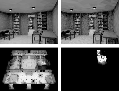
View-importance–driven stochastic Jacobi radiosity. The top images have been obtained using approximately the same total amount of work (3.3 10 rays, under 1 minute of computation time). The top left image, computed with view importance, is significantly less noisy than the top right image, which has been obtained without computing and taking advantage of view importance. The bottom left image shows an overview of the scene in which the view was taken. The scene was subdivided into 162,000 patches. The bottom-right image shows the importance distribution for the view. High intensity indicates high view importance. The model shown is an edited part of the Soda Hall VRML model, available from the University of California at Berkeley.
This requires a measure for the importance of the illumination across the surfaces in the scene. As explained in Section 6.4.3, the adjoints of the radiosity system of equations yield such a measure. Here, it will be more convenient to use adjoints of the power system of equations (Equation (6.8):
The importance Ii is always defined with regard to some direct importance distribution Vi. When choosing Vi = 1 for the patches i that are visible in a view and Vi = 0 for patches that are not visible in a view, Ii is called view importance and indicates what fraction of the radiosity Bi will be contributed to the patches visible in a view, directly or via interreflections.
A continuous view-importance function I(x) on the surfaces of the scene can be defined in a very similar way by means of adjoints of the radiosity integral equation (Equation 6.3):
The equations from which importance is to be solved are of the same form as the equations that describe light transport, and therefore the same algorithms as for light transport can be used for computing importance in a scene. This can happen either in separate phases or at the same time. Moreover, the computation of importance can possibly be sped up by taking advantage of the adjoint of importance: the radiosity. In practice, one should take care that importance is only used for computing radiosity (and vice versa) if the importance solution is sufficiently stable.
View-Importance-Driven Shooting Random Walks
View importance Ii can be used in various ways during random walk sampling:
- For modulating the transition probabilities, so that random walks are scattered preferentially towards regions of high importance. Unfortunately, this can no longer be done using uniformly distributed local or global lines and requires that incoming importance at every patch is stored or can be queried efficiently in some way [103, 192].
- For modulating the survival probabilities only, so particles near important regions get a higher chance of survival. In regions of low importance, particles will be killed off with a higher probability than according to the reflectivity (Russian roulette). In interesting regions, it is even possible to split a particle into two or more new particles of which the scores are appropriately combined (splitting).
- For modulating the birth probabilities, so that more random walks are started from important light sources and fewer from unimportant sources. This can be combined with importance-modulated transition sampling or can be done with analog transition sampling. In the latter case, the best results are obtained by modulating the analog birth probabilities at light sources (proportional to self-emitted power) by the square root of view importance [163].
In order to keep the estimation unbiased, scores shall be decreased when probabilities are increased and vice versa. If the survival chance of a particle is reduced in Russian roulette, for instance, the contribution of a particle that survives the test shall be increased in order to compensate. View-importance-based sampling has been studied for continuous as well as discrete random walks [140, 42, 163, 158, 15].
View-Importance-Driven Stochastic Relaxation Radiosity
In the context of incremental and regular power shooting (Section 6.3.2), view importance can be used to:
- Aim particles preferentially towards interesting regions. The problem is the same as with random walks: local or global line sampling is no longer helpful, and incoming importance needs to be stored with each patch.
- Increase or decrease the probability of shooting a ray from a given patch: this yields the same effect as Russian roulette, splitting and modulating birth probabilities together in random walks. It is very easy to implement with local line sampling.
In general, view-importance-driven stochastic relaxation methods can be derived in exactly the same way as analog stochastic relaxation methods by considering the power system of equations (Equation 6.8) modified as
Non-view-importance-driven stochastic relaxation radiosity corresponds with the choices Ii = 1/ρi and Vi = 1/ρi — 1 (these choices are always a valid solution of Equation 6.28 in closed environments). Figure 6.24 shows some results, obtained with algorithms developed by Neumann and Bekaert [126, 15].
6.6.2 Control Variates
Recall that the main idea of control variate variance reduction (Section 3.6.6) is as follows. Suppose a function f(x) is to be numerically integrated and that we know the integral G of a similar function g(x). If the difference f(x) – g(x) is to good approximation constant, it will be more efficient to use a Monte Carlo method for integrating the difference f(x) – g(x) and add G afterwards. The function g(x) is called a control variate. Control variates have been proposed for variance reduction in stochastic ray tracing by Lafortune [101]. We discuss here the application to discrete random walks and stochastic relaxation.
Control Variates for Linear Systems
This idea can be applied to the solution of linear systems (and integral equations) in the following way: Suppose we know an approximation x̃ for the solution x of x = e + Ax. The correction Δx = x – x̃ then fulfills
Proof:
This is true regardless of the error in the approximation x̃. Now suppose Δx is computed using, for instance, a random walk method. The resulting estimate Δx̃ for the correction Δx will not be exact, so that will not be exactly equal to the solution x of the system to be solved, either. However, regardless of the error on the first approximation x̃, the error on the new approximation x̃ is only determined by the error on the computed correction Δx̃! Sometimes, the correction Δx̃ can be estimated more efficiently than x itself.
Constant Control Variates in Random Walk Radiosity
The only choice for x̃ that allows Ax̃ to be calculated analytically in the case of radiosity is the constant choice B̃i = β. With this choice, we get
The question now is how to determine an optimal value for β. Heuristics for choosing β can be derived by minimizing the expected mean square error of random walk estimators. Several crude approximations need to be made, however, and the benefits are not very significant in practice.
Constant Control Variates in Stochastic Relaxation Radiosity
In stochastic Jacobi relaxation, however, constant control variate variance reduction is easier to obtain and more effective. Monte Carlo summation shall be applied to the following modified power equation:
A good value for the control radiosity β can be obtained by numerical optimization of F(β) = ∑s As |Bs – β| [15, 125].
One disadvantage of constant control variates in radiosity is that the scene being rendered needs to fulfill certain requirements:
- It needs to be closed, because otherwise ∑j Fijβ ≠ β for some patches i in the scene.
- There cannot be closed “holes” in a scene that do not receive any light, e.g., the interior of a box.
The speed-up that can be obtained with a constant control variate typically is in the range of 5-50%.
6.6.3 Gathering for Free
If more than one Monte Carlo estimator is at hand for a given quantity, their combination can also reduce variance considerably. In Monte Carlo radiosity in particular, one will always find a gathering estimator corresponding with each shooting estimator. Gathering is, in general, less efficient than shooting except on small patches, but by combining gathering and shooting over random walks and rays sampled for shooting, variance reduction is possible at negligible additional cost.
Recall that there are basically two ways to combine estimators (see Section 3.6.5).
The classic way. The classic way of combining two estimators Ŝ1 and Ŝ2 for a quantity S is based on the observation that any linear combination w1Ŝ1 + w2Ŝ2 with constant weights w1 + w2 = 1 will also be an unbiased estimator for S. For independent estimators, the optimal combination weights can be shown to be inversely proportional to the variance:
In practice, the weights can be obtained in two different ways:
- Using analytical expressions for the variance of the involved estimators (such as presented in this text).
- Using a posteriori estimates for the variances based on the samples in an experiment themselves (Section 3.4.5). By doing so, a slight bias is introduced. As the number of samples is increased, the bias vanishes: the combination is asymptotically unbiased or consistent.
In general, the combination of M estimators, with Nm samples each, looks like
Multiple importance sampling. It is neither necessary, nor optimal, to take the combination weights wm the same for all samples. By using potentially different sets of weights wmk for each sample k, more robust combination will often be possible:
The result is unbiased as long as for every sample.
An often-used heuristic for choosing the combination weights is the balance heuristic. With this heuristic, the weights wmk are chosen proportional to the probability that the sample k would be generated with the mth technique Ŝm times Nm.
Combining Gathering and Shooting in Discrete Random Walk Radiosity
Combining gathering and shooting over a single set of random walks can be done in several ways:
Using multiple importance sampling. The basic observation is that gathering radiosity over a path segment jt,jt+1, . . . ,js is identical to shooting power over the reverse segment js, js−1, . . . ,jt. Multiple importance sampling can be applied if the probability of having a subpath originating at the endpoints jt and js are both known. In practice, combined gathering and shooting based on multiple importance sampling is useful only with global lines, in global multipath algorithms [157, 161]. With local lines, the required probabilities are unfortunately not known in advance.
Using a posteriori variance estimates. Such estimates can be obtained by approximating analytical expressions [159]. Alternatively, sample-based variance estimation is also possible [15]. Sample-based variance estimation yields very good weights eventually, but the weights are unreliable in the beginning of the computations, when only few random walks have been visiting a patch. A posteriori variance estimation allows us to combine shooting and gathering also with local line sampling. Figure 6.25 shows the shooting and gathering contributions associated with a single path.
Combining gathering and shooting in random walk radiosity yields moderate variance reduction, again 5–50%, but the additional computation cost is negligible.
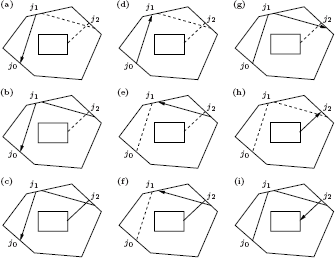
The main idea of “gathering for free.” A single random walk j0, j1, j2, j3 yields multiple scores, which are combined in a provable good way, yielding lower variance at a negligible additional computation cost: (a, b, c) gathering at j0; (d) shooting at j1; (e, f) gathering at j1; (g) shooting at j2; (h) gathering at j2; and (i) shooting at j3.
Combining Gathering and Shooting in Stochastic Jacobi Radiosity
Combining gathering and shooting in stochastic Jacobi iterations is again very simple [15]. Each line shot in power-shooting iterations (Section 6.3.2) yields a contribution to the patch that it hits, while in gathering iterations, the line yields a contribution to the patch from where it was shot. Also here, gathering corresponds with shooting over the reverse line. Unlike with random walks, the probability of shooting a line from every patch is known, so multiple importance sampling can be used. The result is that a score can be recorded at both ends of each shot line. For a line connecting the patches i and j, the scores at both endpoints are
As before, pi and pj indicate the probability of shooting a line from i and j. With local lines, we can choose pi proportional to the power to be shot from i. With global lines, pi is proportional to the patch area Ai.
The technique is extremely simple to implement, it is always safe to use, it comes at no additional cost, and can yield fair speed-ups: up to a factor of 2.
In Section 7.3, we will discuss bidirectional path tracing. Bidirectional path tracing combines light tracing and path tracing (Chapter 5), which are also a pair of shooting and corresponding gathering algorithms. The techniques just described use single shooting or gathering paths for shooting and gathering at the same time. In bidirectional path tracing, separate pairs of a shooting path and a gathering path will be combined.
6.6.4 Weighted Importance Sampling
The basic idea of weighted importance sampling can be explained intuitively as follows: Suppose one needs to compute an integral F = ∫ f(x)dx and that one knows a second, similar, integral G = ∫ g(x)dx with the same domain. Both integrals can then be estimated using the same samples. The resulting Monte Carlo estimate G̃ for G can then be compared with the true, known value of G. Due to its random nature, the estimate G̃ will sometimes be larger than G and sometimes be smaller. Suppose that one knows that the corresponding estimate F̃ for F will also be larger than F in case G̃ is larger than G, a more accurate estimate for F than may be F̃G/̃G: F is decreased if G > G and it is increased if G̃ < G. In short, weighted importance sampling is a multiplicative rather than an additive control variate variance reduction technique.
Unlike the variance reduction techniques described before, weighted importance sampling is biased, but it is consistent if f and g fulfill certain requirements. The bias vanishes as 1/N (N is the number of samples). This is much faster than the statistical error, which vanishes as . A more elaborate exposition of this idea, with application to form factor integration and stochastic relaxation radiosity can be found in [14].
6.6.5 Low-Discrepancy Sampling
As discussed in Section 3.6.7, it is often possible to obtain convergence rates considerably faster than ?() by using low-discrepancy sampling [132]. The main idea of low-discrepancy sampling is to use sample number sequences that are more uniform than random numbers.5 Integration using low-discrepancy number sequences is also called quasi-Monte Carlo integration. Unlike Monte Carlo integration, which is based on statistics, quasi–Monte Carlo methods have a very different origin, in number theory.
In practice, however, improved convergence rates are often obtained by little more than replacing the random number generator by a low-discrepancy number sequence. Local line sampling (Section 6.2.3), for instance, requires four-dimensional random vectors: two random numbers are needed for choosing a ray origin and two more for sampling a cosine-distributed direction. Keller [89] showed that using four-dimensional low-discrepancy vectors instead yields speed-ups of about an order of magnitude when computing form factors with local lines. Neumann et al. observed a similar speed-up when using quasi-random numbers instead of random numbers in stochastic relaxation radiosity [127]. The speed-up obtained with quasi-random sampling in continuous shooting random walk radiosity [90] is much smaller. In discrete shooting random walk radiosity, it is of the same magnitude as in stochastic relaxation radiosity, and often much higher than in continuous random walks [15]. A theoretical study of the convergence rate of quasi-random sampling in radiosity has been carried out by Szirmay-Kalos [190].
There are several important differences between random and quasi-random sampling. The main difference in practice is that quasi-random samples are not statistically independent. They can even be very strongly correlated, leading to disturbing aliasing patterns. Fortunately, there exist very simple and effective techniques to break these correlations, while still maintaining fast convergence [96, 127].
6.7 Hierarchical Refinement and Clustering
All mesh-based algorithms covered so far in this chapter share a common drawback, illustrated in Figure 6.26. If patches are chosen too small, variance will be high. If they are chosen too large, however, disturbing discretization artifacts, such as too smooth illumination and blurred shadow boundaries, result. We discuss here how hierarchical refinement [30], [64], [164] and clustering [182, 174] can be incorporated in stochastic radiosity algorithms. Doing so significantly reduces these problems and considerably boosts the performance of stochastic radiosity algorithms.
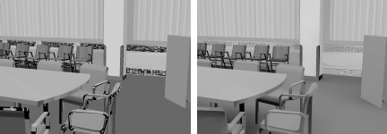
The left image illustrates meshing difficulties with stochastic radiosity. On the one hand, high variance on small patches leads to disturbing noisy artifacts: some of these patches will receive no rays, so that they will be rendered black, while other small patches appear overly bright. Large patches, such as the walls and floor in this image, for instance, appear too smooth as only a single radiosity value is computed for the whole patch. Adaptive meshing, hierarchical refinement, and clustering reduce these problems (right image).
(The conference room model shown is by Anat Grynberg and Greg Ward, Lawrence Berkeley Laboratory, Berkeley, California).
Hierarchical refinement and clustering have been introduced in radiosity with two goals in mind: automatic, adaptive meshing and a reduction of the number of form factors. First, it splits up large patches into smaller ones so that a more accurate radiosity solution is obtained where necessary. Collections of small patches, on the other hand, can also be grouped into single cluster elements behaving like a larger patch. The second key idea is to compute a multiresolution representation of radiosity. A so-called oracle function predicts whether or not light transport can be computed accurately enough between a given pair of elements (patches or clusters) in this multiresolution representation. It ensures that light transport will always be computed at the right level of detail. Doing so leads to significant reduction of the number of form factors to be computed compared to the classic radiosity method: ?(N log N) rather than ?(N2), with N the number of patches.
Adaptive meshing has been integrated with local line form factor computation (Section 6.2.3) by several authors [106], [94], [92]. The basic idea in these three proposals is identical: A large number of rays is shot from the source patch. The surrounding scene is subdivided into receiver elements so that each receiver element (a surface or cluster) receives the same number of rays. The disadvantage is that these techniques will only work if a large number of rays is shot simultaneously from the shooting patch. This is not the case in more recent stochastic relaxation algorithms.
Tobler et al. [197] have presented an adaptive meshing scheme for the histogram method (Section 6.5.2). By simultaneously keeping track of incident particles on successive hierarchical element levels, smoothness assumption violations can be detected. Also, Myszkowski et al. have proposed adaptive meshing for the histogram method [121].
A truly multiresolution Monte Carlo radiosity algorithm was proposed in [12]. The basic observation is that each line cast in nonhierarchical stochastic Jacobi radiosity carries some light flux from the patch containing its origin to the patch containing its destination point (see Figure 6.27). With hierarchical refinement, a whole stack of elements is located at both endpoints. The same refinement oracles as in deterministic hierarchical radiosity can be used in order to predict for each cast line, at what level of the element stack containing the destination point of a line, the flux carried by the line shall be deposited. Elements are refined lazily, on the fly during the computations.
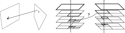
Per-ray hierarchical refinement in stochastic Jacobi radiosity. For each ray shot, connecting two points x and y, the algorithm will determine which level of the element hierarchies at x and y is appropriate for computing light transport from x to y. The element hierarchies are lazily constructed. In non-hierarchical Monte Carlo radiosity, light transport would always be computed between the top-level patches containing the endpoints x and y of the ray.
Per-ray refinement works extremely well with a cheap oracle, such as based on transported power [64]. Some results are presented in Figure 6.28. Hierarchical stochastic Jacobi radiosity has been used in order to rapidly compute radiosity solutions in scenes containing millions of polygons, such as entire building and car models, on commodity PCs.
![Figure showing images rendered with hierarchical Monte Carlo radiosity [12]. The number of elements in the shown images varies from 88,000 (theater) to more than 500,000 (cubicle office space). The radiosity computations for these images took less than 1 minute on a 2GHz Pentium-4 PC with 256MB of RAM. Once computed, the illuminated model can be rendered from new viewpoints in real time, using a low-cost PC three-dimensional graphics accelerator. Model credits: Candlestick Theater. Design: Mark Mack Architects. Three-dimensional model: Charles Ehrlich and Greg Ward (work conducted as a research project during the Architecture 239X course taught by Kevin Matthews formerly at UC Berkeley, College of Environmental Design). Conference room and cubicle space models by Anat Grynberg and Greg Ward.](http://imgdetail.ebookreading.net/software_development/6/9781439864951/9781439864951__advanced-global-illumination__9781439864951__image__213x001.png)
Images rendered with hierarchical Monte Carlo radiosity [12]. The number of elements in the shown images varies from 88,000 (theater) to more than 500,000 (cubicle office space). The radiosity computations for these images took less than 1 minute on a 2GHz Pentium-4 PC with 256MB of RAM. Once computed, the illuminated model can be rendered from new viewpoints in real time, using a low-cost PC three-dimensional graphics accelerator.
Model credits: Candlestick Theater. Design: Mark Mack Architects. Three-dimensional model: Charles Ehrlich and Greg Ward (work conducted as a research project during the Architecture 239X course taught by Kevin Matthews formerly at UC Berkeley, College of Environmental Design). Conference room and cubicle space models by Anat Grynberg and Greg Ward.
(Courtesy of Lawrence Berkeley Laboratory, Berkeley, California.) (See Plate I.)
6.8 Exercises
Compute the form factor for the following configuration. Two identical rectangular plates are positioned parallel to each other (Figure 6.29). Compute the form factor using Monte Carlo integration and compare with the analytical solution. Make a plot of absolute error as a function of the number of sample lines used. Compare empirically stratified, non-stratified, and low-discrepancy sampling (e.g., Halton or Niederreiter; see Section 3.6.7).
Repeat the Exercise 1, but now the plates are perpendicular to each other (Figure 6.30).
- When comparing the Monte Carlo results of the configurations in Exercises 1 and 2, is there a difference in the convergence speed for the two cases? If there is, explain this difference. If there is no difference in convergence speed, why not?
Given is the scene in Figure 6.31 containing 3 diffuse polygons with diffuse reflectivity values of 0.3, 0.4 and 0.5; and 1 diffuse light source emitting 500 watts, covering the complete ceiling.
Compute the relevant form factors using the analytic expressions given above, and compute the radiosity solution for this scene. You can solve the linear system by hand or use a mathematical software tool.
- Increase the diffuse reflectivity for all surfaces in the scene by 10%. What is the result on the new radiosity values? Do the new radiosity values increase by more or less than 10%.? Why?
- Compare the radiosity solution for the scene given above to a solution that only computes direct illumination (assume all form factors are zero except the ones encoding transport starting at the light source).
- Instead of using analytic form factors, insert the form factors computed with Monte Carlo integration. If the Monte Carlo evaluation of form factors in a general scene results in overestimates for the form factors, what could the resulting effect be for the radiosity algorithm?
- Consider a closed environment (there is no loss of radiative energy), for which the average reflectivity ρaverage over all surfaces is known. Find a general expression for the total amount of emitted and reflected power over all surfaces in the scene.
- Write a basic radiosity program, using deterministic shooting Jacobi iterations for system solution, as explained in Section 6.3.1. Use the local lines approach described in Section 6.2.3 for computing the form factors. Compare with pairwise form factor Monte Carlo integration as in the previous exercises. (Hint: since most of the work in this exercise is in writing the code for reading in a 3D model, for tracing rays, and for displaying images, it is a good idea to start with a simple ray-tracing program and extend that.)
- Adapt the basic radiosity program of the previous exercise to compute radiosity in other ways discussed in the radiosity chapter, for instance:
- Implement stochastic regular shooting, incremental shooting, and regular gathering by means of local lines. Compare empirically.
- Implement and compare local and global line sampling.
- Implement discrete random walk radiosity: compare shooting and gathering, absorption versus survival versus collision sampling.
- Implement photon density estimation algorithms. Compare the histogram method with discrete random walk radiosity. In orthogonal series estimation, compare image quality and computation times with constant, linear, quadratic, and cubic approximation. (Hint: display the resulting images either through ray casting or by means of a fragment shader on a GPU). Experiment with the kernel method comparing a cylindrical, Gaussian, Epanechnikov, and other kernels you find in cited literature.
- Try out view-importance–driven sampling in its variants, control variates, and gathering for free in discrete random walk radiosity and stochastic Jacobi.
- For the math-inclined: Familiarize yourself with variance calculation by starting with some simple cases. For instance, derive the variance of:
- regular gathering stochastic Jacobi radiosity;
- absorption random walk radiosity: compare shooting versus gathering, discrete versus continuous.
- Give an intuitive explanation of why collision random walks are generally more efficient than absorption or survival random walks.
- Give an intuitive explanation of why shooting is generally more efficient than gathering.
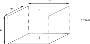
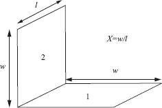
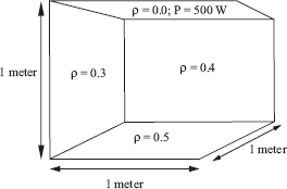
1Similar algorithms based on global line sampling have been proposed as well [157, 161].
2Note that the sum is over the sample points, while division is by the number of photon trajectories!
3In practice, the chance is not zero because of finite-precision arithmetic.
4Adjoint radiosity systems (Equation 6.20) are obtained by multiplying the left- and right-hand side of Equation 6.28 with the patch area Ai. Yi and Wi in Equation 6.20 are related to Ii and Vi here as Yi = AiIi and Wi = AiVi.
5Numbers generated with so-called random number algorithms are not truly random. They merely pass a certain set of statistical tests that truly random numbers would pass as well. Truly random numbers can only be generated with specialized electronic devices (or on certain defective computer equipment).