
Chapter 5
Stochastic Path-Tracing Algorithms
This chapter discusses a class of algorithms for computing global illumination pictures known as path-tracing algorithms1. The common aspect of these algorithms is that they generate light transport paths between light sources and the points in the scene for which we want to compute radiance values. Another, although less vital, characteristic is that they usually compute radiance values for each individual pixel directly. As such, these algorithms are pixel-driven, but many of the principles outlined here can be equally applied to other classes of light transport algorithms, such as finite element techniques (to be discussed in the next chapter).
First, we present a brief history of path-tracing algorithms in the context of global illumination algorithms (Section 5.1). Then, we discuss the camera set-up that is common to most pixel-driven rendering algorithms (Section 5.2) and introduce a simple path-tracing algorithm in Section 5.3. In Section 5.4, we introduce various methods for computing the direct illumination in a scene, followed by similar sections for the special case of environment map illumination (Section 5.5) and indirect illumination (Section 5.6). Finally, in Section 5.7, the light-tracing algorithm is discussed, which is the dual algorithm of ray tracing.
5.1 Brief History
Path-tracing algorithms for global illumination solutions started with the seminal paper on ray tracing by Whitted [194]. This paper described a novel way for extending the ray-casting algorithm to determine visible surfaces in a scene [4] to include perfect specular reflections and refractions. At the time, ray tracing was a very slow algorithm due to the number of rays that had to be traced through the scene, such that many techniques were developed for speeding up the ray-scene intersection test (see [52] for a good overview).
In 1984, Cook et al. [34] described stochastic ray tracing. Rays were distributed over several dimensions, such that glossy reflections and refractions, and other effects such as motion blur and depth of field, could be simulated in a coherent framework.
The paper of Kajiya [85] applied ray tracing to the rendering equation, which described the physical transport of light (see Chapter 2). This technique allowed full global illumination effects to be rendered, including all possible interreflections between any types of surfaces.
Other Monte Carlo sampling techniques were applied to the rendering equation, the most complete being bidirectional ray tracing, introduced by Lafortune [100] and Veach [200].
5.2 Ray-Tracing Set-Up
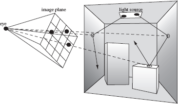
In order to compute a global illumination picture, we need to attribute a radiance value Lpixel to each pixel in the final image. This value is a weighted measure of radiance values incident on the image plane, along a ray coming from the scene, passing through the pixel, and pointing to the eye (Figure 5.1). This is best described by a weighted integral over the image plane:
Lpixel=∫imageplaneL(p→eye)h(p)dp =∫imageplaneL(x→eye)h(p)dp, (5.1)
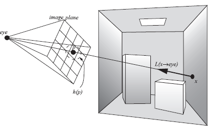
with p being a point on the image plane, and h(p) a weighting or filtering function. x is the visible point seen from the eye through p. Often, h(p) equals a simple box filter such that the final radiance value is computed by uniformly averaging the incident radiance values over the area of the pixel. A more complex camera model is described in [95].
The complete ray-tracing set-up refers to the specific configuration of scene, camera, and pixels, with the specific purpose to compute radiance values for each pixel directly. We need to know the camera position and orientation, and the resolution of the target image. We assume the image is centered along the viewing axis. To evaluate L(p → eye), a ray is cast from the eye through p, in order to find x. Since L(p→eye)=L(x→→xp), we can compute this radiance value using the rendering equation.
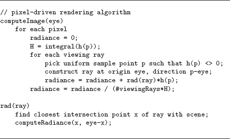
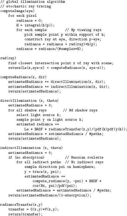
A complete pixel-driven rendering algorithm (see Figure 5.2) consists of a loop over all pixels, and for each pixel, the integral in the image (Equation 5.1) plane is computed using an appropriate integration rule. A simple Monte Carlo sampling over the image plane where h(p) ≠ 0 can be used. For each sample point p, a primary ray needs to be constructed. The radiance along this primary ray is computed using a function rad(ray). This function finds the intersection point x, and then computes the radiance leaving surface point x in the direction of the eye. The final radiance estimate for the pixel is obtained by averaging over the total number of viewing rays, and taking into account the normalizing factor of the uniform PDF over the integration domain (h(p) ≠ 0).
5.3 Simple Stochastic Ray Tracing
5.3.1 Truly Random Paths
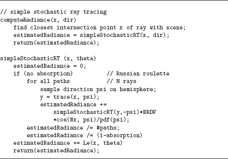
The function compute_radiance(x, eye-x) in the pixel-driven rendering algorithm uses the rendering equation to evaluate the appropriate radiance value. The most simple algorithm to compute this radiance value is to apply a basic and straightforward Monte Carlo integration scheme to the standard form of the rendering equation. Suppose we want to evaluate the radiance L(x → Θ) at some surface point x (Section 2.6):
L(x→Θ)=Le(x→Θ)+Lr(x→Θ) =Le(x→Θ)+∫ΩxL(x←Ψ)fr(x,Θ↔Ψ)cos (Ψ,Nx)dωΨ.
The integral can be evaluated using Monte Carlo integration, by generating N random directions Ψi over the hemisphere Ωx, distributed according to some probability density function p(Ψ). The estimator for Lr(x → Θ) is then given by
〈Lr(x→Θ)〉=1NN∑i=1L(x←Ψi)fr(x,Θ↔Ψi)cos (Ψi,Nx)p(Ψi).
The cosine and BRDF terms in the integrand can be evaluated by accessing the scene description. L(x ← Ψi), the incident radiance at x, is however unknown. Since
L(x←Ψi)=L(r(x,Ψi)→−Ψi),
we need to trace the ray leaving x in direction Ψi through the environment to find the closest intersection point r(x, Ψ). At this point, another radiance evaluation is needed. Thus, we have a recursive procedure to evaluate L(x ← Ψi), and a path, or a tree of paths, is traced through the scene.
Any of these radiance evaluations will only yield a nonzero value if the path hits a surface for which Le is different from 0. In other words, the recursive path needs to hit one of the light sources in the scene. Since the light sources usually are small compared to the other surfaces, this does not occur very often, and very few of the paths will yield a contribution to the radiance value to be computed. The resulting image will mostly be black. Only when a path hits a light source will the corresponding pixel be attributed a color. This is to be expected, since the algorithm generates paths in the scene, starting at the point of interest, and slowly working towards the light sources in a very uncoordinated manner.
In theory, this algorithm could be improved somewhat by choosing p(Ψ) to be proportional to the cosine term or the BRDF, according to the principle of importance sampling (see Section 3.6.1). In practice, the disadvantage of picking up mostly zero-value terms is not changing the result considerably. Note, however, that this simple approach will produce an unbiased image if a sufficient number of paths per pixel are generated.
5.3.2 Russian Roulette
The recursive path generator described in the simple stochastic ray-tracing algorithm needs a stopping condition. Otherwise, the generated paths would be of infinite length and the algorithm would not come to a halt. When adding a stopping condition, one has to be careful not to introduce any bias to the final image. Theoretically, light reflects infinitely in the scene, and we cannot ignore these light paths of a long length, which might be potentially very important. Thus, we have to find a way to limit the length of the paths but still be able to obtain a correct solution.
In classic ray-tracing implementations, two techniques are often used to prevent paths from growing too long. A first technique is cutting off the recursive evaluations after a fixed number of evaluations. In other words, the paths are generated up to a certain specified length. This puts an upper bound on the number of rays that need to be traced, but important light transport might have been ignored. Thus, the image will be biased. A typical fixed path length is set at 4 or 5 but really should be dependent on the scene to be rendered. A scene with many specular surfaces will require a larger path length, while scenes with mostly diffuse surfaces can usually use a shorter path length. Another approach is to use an adaptive cut-off length. When a path hits a light source, the radiance found at the light source still needs to be multiplied by all cosine factors and BRDF evaluations (and divided by all PDF values) at all previous intersection points before it can be added to the final estimate of the radiance through the pixel. This accumulating multiplication factor can be stored along with the lengthening path. If this factor falls below a certain threshold, recursive path generation is stopped. This technique is more efficient compared to the fixed path-length, because many paths will be stopped before, and fewer errors are made, but the final image will still be biased.
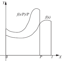
Russian roulette is a technique that addresses the problem of keeping the lengths of the paths manageable but at the same time leaves room for exploring all possible paths of any length. Thus, an unbiased image can still be produced. To explain the Russian roulette principle, let us look at a simple example first. Suppose we want to compute the following one-dimensional integral:
I=∫10f(x)dx.
The standard Monte Carlo integration procedure generates random points xi in the domain [0, 1] and computes the weighted average of all function values f(xi). Assume that for some reason f(x) is difficult or complex to evaluate (e.g., f(x) might be expressed as another integral), and we would like to limit the number of evaluations of f(x) necessary to estimate I. By scaling f(x) by a factor of P horizontally and a factor of 1/P vertically, we can also express the quantity I as
IRR=∫P01Pf(xP)dx,
with P ≤ 1. Applying Monte Carlo integration to compute the new integral, using a unform PDF p(x) = 1 to generate the samples over [0,1], we get the following estimator for IRR:
〈IRR〉={1Pf(xP)if x≤ P0if x > P.
It is easy to verify that the expected value of 〈IRR〉 equals I. If f(x) would be another recursive integral (as is the case in the rendering equation), the result of applying Russian roulette is that recursion stops with a probability equal to α = 1 — P for each evaluation point. α is called the absorption probability. Samples generated in the interval [P, 1] will generate a function value equal to 0, but this is compensated by weighting the samples in [0, P] with a factor 1/P. Thus, the overall estimator still remains unbiased.
If α is small, the recursion will continue many times, and the final estimator will be more accurate. If α is large, the recursion will stop sooner, but the estimator will have a higher variance. For our simple path-tracing algorithm, this means that either we generate accurate paths having a long length, or very short paths, which provide a less accurate estimate. However, the final estimator will be unbiased.
In principle, we can pick any value for α, and we can control the execution time of the algorithm by picking an appropriate value. In global illumination algorithms, it is common for 1 — a to be equal to the hemispherical reflectance of the material of the surface. Thus, dark surfaces will absorb the path more easily, while lighter surfaces have a higher chance of reflecting the path. This corresponds to the physical behavior of light incident on these surfaces.
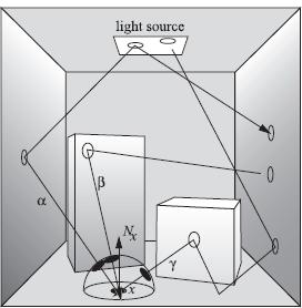
The complete algorithm for simple stochastic ray tracing is given in Figure 5.4 and is illustrated in Figure 5.5. Paths are traced starting at point x. Path α contributes to the radiance estimate at x, since it reflects off the light source at the second reflection and is absorbed afterwards. Path γ also contributes, even though it is absorbed at the light source. Path β does not contribute, since it gets absorbed before reaching the light source.
5.4 Direct Illumination
The simple stochastic path tracer described in Section 5.3 is rather inefficient, since directions around each surface point are sampled without taking the position of the light sources into account. It is obvious that light sources contribute significantly to the illumination of any surface point visible to them. By sending paths to the light sources explicitly, accurate pictures are obtained much faster.
5.4.1 Direct and Indirect Illumination
As explained in Section 2.6, the reflected radiance term of the rendering equation can be split into two parts: a term that describes the direct illumination due to the light sources and one that describes the indirect illumination. We first write the reflected radiance integral using exitant radiance only:
Lr(x→Θ)=∫ΩxL(x←Ψ)fr(x,Θ↔Ψ,Nx)dωΨ =∫ΩxL(r(x,Ψ)→−Ψ)fr(x,Θ↔Ψ)cos (Ψ,Nx)dωΨ.
Rewriting L(r(x, Ψ) → — Ψ) as a sum of self-emitted and reflected radiance at r(x, Ψ) gives us
Lr(x→Θ)=∫ΩxLe(r(x,Ψ)→−Ψ)fr(x,Θ↔Ψ)cos (Ψ,Nx)dωΨ+∫ΩxLr(r(x,Ψ)→−Ψ)fr(x,Θ↔Ψ)cos (Ψ,Nx)dωΨ =Ldirect(x→Θ)+Lindirect(x→Θ). (5.2)
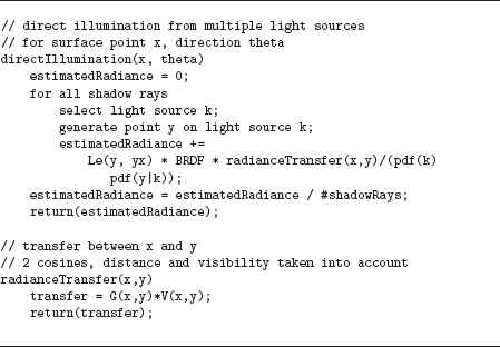
The direct term Ldirect(x → Θ) expresses the contribution to Lr(x → Θ) directly from the light sources. Since the integrand of Ldirect(x → Θ) contains Le(r(x, Ψ) → — Ψ), which only differs from zero at the light sources, we can transform the hemispherical integral to an integral over the area of the light sources only (Figure 5.6),

Ldirect(x→Θ)=∫AsourcesLe(y→→yx)fr(x,Θ↔→xy)G(x,y)V(x,y)dAy, (5.3)
or by explicitly summing over all NL light sources in the scene,
Ldirect(x→Θ)=NL∑k=1∫AkLe(y→→yx)fr(x,Θ↔→xy)G(x,y)V(x,y)dAy.
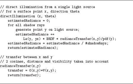
This integral over all light sources can now be computed using a very efficient sampling scheme. By generating surface points on the area of the light sources, we are sure that, if the light source is visible to the point x, a nonzero contribution is added to the Monte Carlo estimator for x. If x is in a shadow, the contribution to the estimator equals 0.
There are two options to sample surface points on the light sources: we can compute the direct illumination for each light source separately or we can consider the combined light sources as one large light source, treating it as a single integration domain. Surface points yi on the light sources will be generated, and for each sample yi, the integrand Le(yi → x) fr(x,Θ↔→xyi)G(x,yi)V(x,yi) has to be evaluated. Since V(x, yi) requires a visibility check and represents whether the point x is in shadow relative to yi, the paths generated between x and yi are often called shadow rays.
The following choices of settings will determine the accuracy of the direct illumination computation:
- Total number of shadow rays. Increasing the number of shadow rays will produce a better estimate.
- Shadow rays per light source. According to the principle of importance sampling, the number of shadow rays per light source should be proportional to the relative contribution of the light source to the illumination of x.
- Distribution of shadow rays within a light source. More shadow rays should be generated for the parts of the light source that have a greater impact on the direct illumination. For example, large area light sources will have areas that are close to the surface points to be illuminated. These areas should receive more shadow rays to obtain a more accurate estimator for direct illumination.
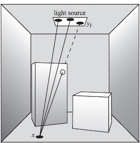
5.4.2 Single Light Source Illumination
To compute the direct illumination due to a single light source in the scene, i.e., a light source that consists of one continuous area, we need to define a probability density function P(y) over the area of the light source, which generates the shadow rays. We assume that such a PDF can be constructed, irrespective of the geometrical nature of the light source.
Applying Monte Carlo integration (using NS shadow rays) to Equation 5.3 yields the following estimator:
〈Ldirect(x→Θ)〉=1NsNs∑i=1Le(yi→→yix)fr(x,Θ↔→xyi)G(x,yi)V(x,yi)p(yi).
For each surface point yi sampled on the light source, the energy transfer between yi and x needs to be computed. This requires evaluations of the BRDF at x, a visibility check between x and yi, the geometric coupling factor, and the emitted radiance at yi. The whole energy transfer has to be weighted by p(yi). An overview of the sampling procedure is given in Figure 5.7.
The variance of this Monte Carlo integration, and thus the noise in the final image, is mainly determined by the choice of p(y). Ideally, p(y) equals the contribution each point y contributes to the final estimator, but in practice, this is almost never possible, and more pragmatic choices have to be made, mainly driven by ease of implementation. Interesting, and often used, choices for p(y) are:
Uniform sampling of light source area. In this case, the points yi are distributed uniformly over the area of the light source, and p(y) = 1/Asource. This is the easiest way of sampling a light source, and optimizations such as stratified sampling can easily be used (Figure 5.8). Using this sampling scheme, there are several sources of noise in the image. If a point x is located in the penumbra region of a shadow, some of its shadow rays will yield V (x, yi) = 0, and some will not. This causes most of the noise in these soft-shadowed areas. On the other hand, if x is located outside any shadow area, all the noise is caused in variations of the cosine terms, but most importantly, variations in 1/r2xy. This is especially noticeable if the light sources are large. The pictures in Figure 5.9 show a simple scene rendered with 1, 9, 36, and 100 shadow rays, respectively. For each pixel, a single viewing ray is cast through the center of the pixel, which produces the closest intersection point x for which a radiance value needs to be computed. It is obvious that when only one shadow ray is used, surface points either lie in shadow or are visible for the light source. Some pixels in which the penumbra is visible are therefore completely black, hence, the high amount of noise in the soft shadow regions.
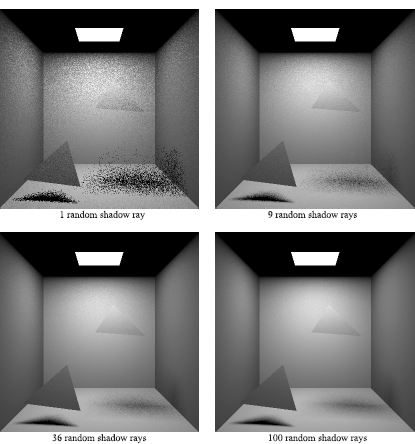
Uniform light source sampling. The images are generated with 1 viewing ray per pixel and 1, 9, 36, and 100 shadow rays. The difference in quality between soft shadows and hard shadows is noticeable.
Uniform sampling of solid angle subtended by light source. To eliminate noise caused by either the cosine terms or the inverse distance squared factor, sampling according to solid angle is an option. This requires rewriting the integral over the area of the light source as an integral over the solid angle subtended by the light source. This would remove one cosine term and the distance factor from the integrand. However, the visibility term is still present. This sampling procedure is useful for light sources that have a significant foreshortening with regard to x, making sure these important areas are not undersampled. This sampling technique is usually difficult to implement, since generating directions over an arbitrary solid angle is not straightforward [6].
Many scenes only contain diffuse light sources, and thus Le(y→→yx) does not add to any noise in the estimation of Ldirect(x → Θ). If the light source is nondiffuse, Le(y→→yx) is not a constant function. There might be areas or directions of the light source emission pattern that are much brighter than others. It could be useful to apply importance sampling based on the emission term, but in practice, this is difficult, since only directions towards x need to be considered. However, a spatially variant light source thbat is diffuse in its angular component could be importance-sampled, reducing variance.
5.4.3 Multiple Light Source Illumination
When there are multiple light sources in the scene, the most simple way is to compute the direct illumination separately for each of the light sources in turn. We generate a number of shadow rays for each light source and afterwards sum up the total contributions of each source. This way, the direct illumination component of each light source will be computed independently, and the number of shadow rays for each light source can be chosen according to any criterion (e.g., equal for all light sources, proportional to the total power of the source, proportional to the inverse distance squared between the point and the point x, etc.)
However, it is often better to consider all combined light sources as a single integration domain and apply Monte Carlo integration to the combined integral. When shadow rays are generated, they can be directed to any of the light sources. It is, therefore, possible to compute the direct illumination of any number of light sources with just a single shadow ray and still obtain an unbiased picture (although, in this case, the noise in the final image will probably be very high). This approach works because we make complete abstraction of light sources as separate, disjunct surfaces and just look at the entirety of the integration domain. However, in order to have a working sampling algorithm, we still need access to any of the light sources separately, because any individual light source might require a separate sampling procedure for generating points over its surface.
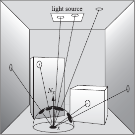
Generally, a two-step sampling process is used for each shadow ray (Figure 5.10):

- First, a discrete probability density function pL(k) is used to select a light sources ki. We assign to each of NL light source a probability value with which it will be chosen to send a shadow ray to. Typically, this probability function is the same for all shadow rays we want to cast but can be different for each different surface point x for which we want to compute a radiance value.
- During the second step, a surface point yi on the light source k selected during the previous step is generated using a conditional PDF p(y|ki). The nature of this PDF is dependent on light source ki. For example, some light sources might be sampled using uniform area sampling, while others might be sampled by generating shadow rays over the subtended solid angle.
The combined PDF for a sampled point yi on the combined area of all light sources is then pL(k)p(y|k). This produces the following estimator for N shadow rays:
〈Ldirect(x→Θ)〉=1NN∑i=1Le(yi→→yix)fr(x,Θ↔→xyi)G(x,yi)V(x,yi)pL(ki)p(yi|ki). (5.4)
Figure 5.11 shows the algorithm for computing the direct illumination due to multiple light sources. Note, however, that the algorithm for computing the illumination due to a single source could be used as well, repeating it for each individual light source.
Although any PDFs pL(k) and p(y|k) will produce unbiased images, the specific choice for which PDFs to use will have an impact on the variance of the estimators and the noise in the final picture. Some of the more popular choices are:
Uniform source selection, uniform sampling of light source area. Both PDFs are uniform: pL(k) = 1/NL and P(y|k) = 1/ALk. Every light source will receive, on average, an equal number of shadow rays, and these shadow rays are distributed uniformly over the area of each light source. This is easy to implement, but the disadvantages are that the illumination of both bright and weak light sources are computed with an equal number of shadow rays and that light sources that are far away or invisible receive an equal number of shadow rays as light sources that are close-by. Thus, the relative importance of each light source is not taken into account. Substituting the PDFs in Equation 5.4 gives the following estimator for the direct illumination:
〈Ldirect(x→Θ)〉=NLNN∑i=1ALkLe(yi→→yix) fr(x,Θ↔→xyi)G(x,yi)V(x,yi).
Power-proportional source selection, uniform sampling of light source area. Here, the PDF pL(k) = Pk/Ptotal with Pk the power of light source k and Ptotal the total power emitted by all light sources. Bright sources would receive more shadow rays, and very dim light sources might receive very few. This is likely to reduce variance and noise in the picture.
〈Ldirect(x→Θ)〉=PtotalNN∑i=1ALkLe(yi→→yix)fr(x,Θ↔→xyi)G(x,yi)V(x,yi)Pk
If all light sources are diffuse, Pk = πAkLe,k, and thus
〈Ldirect(x→Θ)〉=PtotalπNN∑i=1fr(x,Θ↔→xyi)G(x,yi)V(x,yi).
This approach is typically superior since it gives importance to bright sources, but it could result in slower convergence at pixels where the bright lights are invisible and illumination is dominated by less bright lights at these pixels. This latter occurrence can only be solved by using sampling strategies that use some knowledge about the visibility of the light sources.
No matter what pL(k) is chosen, one has to be sure not to exclude any light sources that might contribute to Ldirect(x → Θ). Just dropping small, weak, or faraway light sources might result in bias, and for some portions of the image, this bias can be significant.
One of the drawbacks of the above two-step procedure is that three random numbers are needed to generate a shadow ray: one random number to select the light source k, and two random numbers to select a specific surface point yi within the area of the light source. This makes stratified sampling more difficult to implement. In [170], a technique is described that makes it possible to use only two random numbers when generating shadow rays for a number of disjunct light sources. The two-dimensional integration domain covering all light sources is mapped on the standard two-dimensional unit square. Each light source corresponds to a small subdomain of the unit square. When a point is sampled on the unit square, we find out what subarea it is in, and then transform the location of the point to the actual light source. Sampling in a three-dimensional domain has now been reduced to sampling in a two-dimensional domain, which makes it easier to apply stratified sampling or other variance-reduction techniques.
5.4.4 Alternative Shadow Ray Sampling
Area sampling of the light sources is the most intuitive and best known algorithm for computing direct illumination in a scene. We expect the variance to be low, since knowledge is used in the sampling procedure about where light is coming from in the scene. However, some other sampling techniques can be used to compute the direct illumination, which are often less efficient, but are interesting from a theoretical point of view. These techniques offer alternative ways of constructing paths between the point of interest and the light source.
Shadow rays by hemisphere sampling. This sampling procedure is related to the simple stochastic ray-tracing algorithm, explained in Section 5.3. Directions Ψi are generated over the hemisphere Ωx, after which the nearest intersection point r(x, Ψi) is found. If r(x, Ψi) belongs to a light source, a contribution to the direct illumination estimator is recorded. In Figure 5.12, only two out of seven rays reach the light source and yield a contribution different from 0. This is actually the simple stochastic ray-tracing algorithm, in which the recursion is ended after one level. Many rays will be oriented towards surfaces that are not light sources. The noise and variance are mostly caused by this fact and not by any visibility considerations, since the visibility will not be present in the final estimator. The visibility term is implicitly contained in the computation of the nearest visible point r(x, Ψi).
Shadow rays by global area sampling. The integral describing global illumination (Equation 5.3) integrates over the area of all light sources. It is also possible to write this integral as an integration over all surfaces in the scene, since the self-emitted radiance equals 0 over surfaces that are not a light source (Figure 5.13). Using this formulation, surface points can be sampled over any surface in the scene. The evaluation is the same as for regular shadow rays, except that the Le(yi) factor might be equal to 0, introducing an extra source of noise.
Although these methods do not make much sense from an efficiency point of view, they emphasize the basic principle of computing light transport: paths need to be generated between the light sources and the receiving point. The methods merely differ in how the paths are generated, but this has a drastic impact on the accuracy of their corresponding estimators.
5.4.5 Further Optimizations
Many optimizations have been proposed to make the computation of direct illumination more efficient. Most of these deal with trying to make the evaluation of V (x, y) more efficient, or by preselecting the light sources to which to send shadow rays.
Ward [223] accelerates the direct illumination due to multiple light sources using a user-specified threshold to eliminate lights that are less important. For each pixel in the image, the system sorts the lights according to their maximum possible contribution, assuming the lights are fully visible. Occlusion for each of the largest possible contributors at the pixel is tested, measuring their actual contribution to the pixel and stopping at a predetermined energy threshold. This approach can reduce the number of occlusion tests; however, it does not reduce the cost of occlusion tests that do have to be performed and does not do very well when illumination is uniform.
The approach of Shirley et al. [230] subdivides the scene into voxels and, for each voxel, partitions the set of lights into an important set and an unimportant set. Each light in the important set is sampled explicitly. One light is picked at random from the unimportant set as a representative of the set and sampled. The assumption is that the unimportant lights all contribute the same amount of energy. To determine the set of important lights, they construct an influence box around each light. An influence box contains all points on which the light could contribute more than the threshold amount of energy. This box is intersected with voxels in the scene to determine for which voxels the light is important. This is an effective way to deal with many lights. However, the approach is geared towards producing still images since many samples per pixel are required to reduce the noise inherent in sampling the light set.
Paquette et al. [136] present a light hierarchy for rendering scenes with many lights quickly. This system builds an octree around the set of lights, subdividing until there is less than a predetermined number of lights in each cell. Each octree cell then has a virtual light constructed for it that represents the illumination caused by all the lights within it. They derive error bounds that can determine when it is appropriate to shade a point with a particular virtual light representation and when traversal of the hierarchy to finer levels is necessary. Their algorithm can deal with thousands of point lights. One major limitation of this approach is that it does not take visibility into consideration.
Haines et al. [60] substantially accelerated shadow rays by explicitly keeping track of occluding geometry and storing it in a cube around the light source. However, their technique does not work for area lights and also does no specific acceleration for many lights.
Fernandez et al. [45] use local illumination environments. For each pixel in the image, and for each light source, a list of possible occluders is built adaptively by casting shadow rays. Their technique works well for interactive speeds. Hart et al. [65] use a similar approach, but information about what geometry causes shadows in pixels is distributed in the image using a flood-fill algorithm.
5.5 Environment Map Illumination
The techniques outlined in the previous section are applicable to almost all types of light sources. It is sufficient to choose an appropriate PDF to select one light source from amongst all light sources in the scene, and to choose a PDF to sample a random surface point on the selected light source. The total variance, and hence the stochastic noise in the image, will be highly dependent on the types of PDFs chosen.
Environment maps (sometimes also called illumination maps or reflection maps) are a type of light source that has received significant attention. An environment map encodes the total illumination present on the hemisphere of directions around a single point. Usually, environment maps are captured in natural environments using digital cameras.
An environment map can be described mathematically as a stepwise-continuous function, in which each pixel corresponds to a small solid angle ΔΩ around the point x at which the environment map is centered. The intensity of each pixel then corresponds to an incident radiance value L(x ← Θ), with Θ ∈ ΔΩ.
5.5.1 Capturing Environment Maps
Environment maps usually represent real-world illumination conditions. A light probe in conjunction with a digital camera or a digital camera equipped with a fisheye lens are the most common techniques for capturing environment maps.
Light Probe
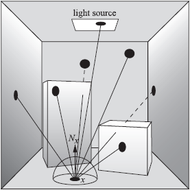
A practical way to acquire an environment map of a real environment is the use of a light probe. A light probe is nothing more than a specular reflective ball that is positioned at the point where the incident illumination needs to be captured. The light probe is subsequently photographed using a camera equipped with an orthographic lens, or alternatively, a large zoom lens such that orthographic conditions are approximated as closely as possible.
The center pixel in the recorded image of the light probe corresponds with a single incident direction. This direction can be computed rather easily, since the normal vector on the light probe is known, and a mapping from pixel coordinates to incident directions can be used. A photograph of the light probe can therefore results in a set of samples L(x ← Θ) (Figure 5.14).

Photographing a light probe produces an environment map representing incident radiance from all directions.
(Photograph courtesy of Vincent Masselus.)
Although the acquisition process is straightforward, there are a number of issues to be considered:
- The camera will be reflected in the light probe and will be present in the photograph, thereby blocking light coming from directions directly behind the camera.
- The use of a light probe does not result in a uniform sampling of directions over the hemisphere. Directions opposite the camera are sampled poorly, whereas directions on the same side of the camera are sampled densely.
- All directions sampled at the edge of the image of the light probe represent illumination from the same direction. Since the light probe has a small radius, these values may differ slightly.
- Since the camera cannot capture all illumination levels due to its nonlinear response curve, a process of high dynamic range photography needs to be used to acquire an environment map that correctly represents radiance values.
Some of these problems can be alleviated by capturing two photographs of the light probe 90 degrees apart. The samples of both photographs can be combined into a single environment map as is shown in Figure 5.15.
Photographing a light probe twice, 90 degrees apart. The camera positions are indicated in blue. Combining both photographs produces a well-sampled environment map without the camera being visible.
(Photographs courtesy of Vincent Masselus.) (See Plate XIX.)
Fisheye Lens
An alternative for capturing an environment map is to make use of a camera equipped with a fisheye lens. Two photographs taken from opposite view directions result in a single environment map as well. However, there are some limitations:
- Good fisheye lenses can be very expensive and hard to calibrate.
- Both images need to be taken in perfect opposite view directions, otherwise a significant set of directions will not be present in the photograph.
If the incident illumination of directions in only one hemisphere needs to be known instead of the full sphere of directions, the use of a fisheye lens can be very practical.
5.5.2 Parameterizations
When using environment maps in global illumination algorithms, they need to be expressed in some parameter space. Various parameterizations can be used, and the effectiveness of how well environments maps can be sampled is dependent on the type of parameterization used. In essence, this is the same choice one has to make when computing the rendering equation as an integral over the hemisphere.
Various types of parameterizations are used in the context of environment maps, and we provide a brief overview here. A more in-depth analysis can be found in [118].
- Latitude-longitude parameterization. This is the same parameterization as the hemispherical coordinate system describes in Appendix A but extended to the full sphere of directions. The advantage is an equal distribution of the tilt angle θ, but there is a singularity around both poles, which are represented as lines in the map. Additional problems are that the pixels in the map do not occupy equal solid angles and that the ϕ = 0 and ϕ = 2π angles are not mapped continuously next to each other (Figure 5.16(a)).
- Projected-disk parameterization. This parameterization is also known as Nusselt embedding. The hemisphere of directions is projected on a disk of radius 1. The advantages are the continuous mapping of the azimuthal angle ϕ, and the pole being a single point in the map. However, the tilt angle θ is nonuniformly distributed over the map (Figure 5.16(b)). A variant is the paraboloid parameterization, in which the tilt angle is distributed more evenly [72] (Figure 5.16(c)).
- Concentric-map parameterization. The concentric map parameterization transforms the projected unit disk to a unit square [165]. This makes sampling of directions in the map easier and keeps the continuity of the projected-disk parameterizations (Figure 5.16(d)).
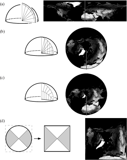
Different parameterizations for the (hemi)sphere: (a) latitudelongitude parameterization; (b) projected-disk parameterization; (c) paraboloid parameterization; (d) concentric-map parameterization.
(Diagrams courtesy of Vincent Masselus.)
5.5.3 Sampling Environment Maps
The direct illumination of a surface point due to an environment map can be expressed as follows:
Ldirect(x→Θ)=∫ΩxLmap(x←Ψ)fr(x,Θ↔Ψ)cos (Ψ,Nx)dωΨ.
The integrand contains the incident illumination Lmap(x ← Ψ) on point x, coming from direction Ψ in the environment map.
Other surfaces present in the scene might prevent the light coming from direction Ψ reaching x. These surfaces might belong to other objects, or the object to which x belongs can cast self-shadows onto x. In these cases, a visibility term V(x, Ψ) has to be added:
Ldirect(x→Θ)=∫ΩxLmap(x←Ψ)fr(x,Θ↔Ψ)V(x,Ψ)cos (Ψ,Nx)dωΨ. (5.5)
A straightforward application of Monte Carlo integration would result in the following estimator:
〈Ldirect(x→Θ)〉=1NN∑i=1Lmap(x←Ψi)fr(x,Θ↔Ψi)V(x,Ψi)cos (Ψi,Nx)p(Ψi),
in which the different sampled directions Ψi are generated directly in the parameterization of the environment map using a PDF p(Ψ).
However, various problems present themselves when trying to approximate this integral using Monte Carlo integration:
- Integration domain. The environment map acting as a light source occupies the complete solid angle around the point to be shaded, and thus, the integration domain of the direct illumination equation has a large extent, usually increasing variance.
- Textured light source. Each pixel in the environment map represents a small solid angle of incident light. The environment map can therefore be considered as a textured light source. The radiance distribution in the environment map can contain high frequencies or discontinuities, thereby again increasing variance and stochastic noise in the final image. Especially when capturing effects such as the sun or bright windows, very high peaks of illumination values can be present in the environment map.
- Product of environment map and BRDF. As expressed in Equation 5.5, the integrand contains the product of the incident illumination Lmap(x ← Ψ) and the BRDF fr(x, Θ ↔ Ψ). In addition to the discontinuities and high-frequency effects present in the environment map, a glossy or specular BRDF also contains very sharp peaks. These peaks on the sphere or hemisphere of directions for both illumination values and BRDF values are usually not located at the same directions. This makes it very difficult to design a very efficient sample scheme that takes these features into account.
- Visibility. If the visibility term is included, additional discontinuities are present in the integrand. This is very similar to the handling of the visibility term in standard direct illumination computations but might complicate an efficient sampling process.
Practical approaches try to construct a PDF p(Ψ) that addresses these problems. Roughly, these can be divided in three categories: PDFs based on the distribution of radiance values Lmap(x ← Ψ) in the illumination map only, usually taking into account cos(Ψ, Nx) that can be pre-multiplied into the illumination map; PDFs based on the BRDF fr(x, Θ ↔ Ψ), which are especially useful if the BRDF is of a glossy or specular nature; and PDFs based on the product of both functions, but which are usually harder to construct.
Direct illumination map sampling. A first approach for constructing a PDF based on the radiance values in the illumination map can be simply to transform the piecewise-constant pixel values into a PDF by computing the cumulative distribution in two dimensions and subsequently inverting it. This typically results in a 2D look-up table, and the efficiency of the method is highly dependent on how fast this look-up table can be queried.
A different approach is to simplify the environment map by transforming it to a number of well-selected point light sources. This has the advantage that there is a consistent sampling of the environment map for all surface points to be shaded, but can possibly introduce aliasing artifacts, especially when using a low number of light sources. In [97], an approach is presented in which a quadrature rule is generated automatically from a high dynamic range environment map. Visibility is taken into account in the structured importance sampling algorithm, in which the environment map is subdivided into a number of cells [1].
BRDF sampling. The main disadvantage of constructing a PDF based only on the illumination map is that the BRDF is not included in the sampling process but is left to be evaluated after the sample directions have been chosen. This is particularly problematic for specular and glossy BRDFs, and if this is the case, a PDF based on the BRDF will produce better results.
This of course requires that the BRDF can be sampled analytically, which is not always possible, except for a few well-constructed BRDFs (e.g., a Phong BRDF or Lafortune BRDF). Otherwise, the inverse cumulative distribution technique will have to be used for the BRDF as well.
- Sampling the product. The best approach is to construct a sampling scheme based on the product of both the illumination map and the BRDF, possibly including the cosine and some visibility information as well. In [21], bidirectional importance sampling is introduced, which constructs a sampling procedure based on rejection sampling. The disadvantage is that it is difficult to predict exactly how many samples will be rejected, and hence the computation time. Resampled importance sampling is a variant of this approach [195]. Wavelet importance sampling [27] constructs a PDF based on the wavelet representation of both the illumination map and the BRDF, but this implies some restrictions on what type of map and BRDF can be used.
5.6 Indirect Illumination
This section deals with the computation of indirect illumination in a scene. As opposed to direct illumination computations, this problem is usually much harder, since indirect light might reach a surface point x from all possible directions. For this reason, it is very hard to optimize the indirect illumination computations along the same lines as was done for direct illumination.
Indirect illumination consists of the light reaching a target point x after at least one reflection at an intermediate surface between the light sources and x. The indirect illumination is a very important component of the total light distribution in a scene and usually takes the largest amount of work in any global illumination algorithm. A realistic rendering of the indirect illumination is often necessary to judge any computer-generated picture as being photorealistic.
5.6.1 Uniform Sampling for Indirect Illumination
In Section 5.4.1, the rendering equation was split into a direct and indirect part. The indirect illumination contribution to L(x → Θ) is expressed as
Lindirect(x→Θ)=∫ΩxLr(r(x,Ψ)→−Ψ)fr(x,Θ↔Ψ)cos (Ψ,Nx)dωΨ.
The integrand contains the reflected radiances Lr from other points in the scene, which are themselves composed of a direct and indirect illumination part (according to Equation 5.2). Unlike what was done with the direct illumination equation, we cannot reformulate this integral to a smaller integration domain. Lr(r(x, Ψ) → — Ψ) has (in a closed environment) a nonzero value for all (x, Ψ) pairs. So, the entire hemisphere needs to be considered as the integration domain and needs to be sampled accordingly.
The most general Monte Carlo procedure to evaluate the indirect illumination is to use an arbitrary, hemispherical PDF p(Ψ) and to generate N random directions Ψi. This produces the following estimator:
〈Ldirect(x→Θ)〉=1NN∑i=1Lr(r(x,Ψi)→−Ψi)fr(x,Θ↔Ψi)cos (Ψi,Nx)p(Ψi).
To evaluate this estimator, for each generated direction Ψi, we need to evaluate the BRDF and the cosine term, trace a ray from x in the direction of Ψi, and evaluate the reflected radiance Lr(r(x, Ψi) → —Ψi) at the closest intersection point r(x, Ψi). This last evaluation shows the recursive nature of indirect illumination, since this reflected radiance at r(x, Ψi) can be split again into a direct and indirect contribution. The algorithm for evaluating the indirect illumination is given in Figure 5.17 and graphically shown in Figure 5.18.

Paths generated during indirect illumination computations. Shadow rays for direct illumination are shown as dashed lines.
The recursive evaluation can be stopped using Russian roulette, in the same way as was done for simple stochastic ray tracing. Generally, the local hemispherical reflectance is used as an appropriate absorption probability. This choice can be explained intuitively: we only want to spend work (i.e., tracing rays and evaluating Lindirect(x)) proportional to the amount of energy present in different parts of the scene.
5.6.2 Importance Sampling for Indirect Illumination
The simplest choice for p(Ψ) is a uniform PDF p(Ψ) = 1/2π, such that directions are sampled proportional to solid angles. This is easy and straightforward to implement. Noise in the resulting picture will be caused by variations in the BRDF and cosine evaluations, and variations in the reflected radiance Lr at the distant points.
Uniform sampling over the hemisphere does not take into account any knowledge we might have about the integrand in the indirect illumination integral. In order to reduce noise, some form of importance sampling is needed. We can construct a hemispherical PDF proportional (or approximately proportional) to any of the following factors:
- The cosine factor cos(Ψi, Nx).
- The BRDF fr(x,Θ ↔ Ψi).
- The incident radiance field Lr(r(x,Ψi).
- A combination of any of the above.
Cosine Sampling
Sampling directions proportional to the cosine lobe around the normal Nx prevents too many directions from being sampled near the horizon of the hemisphere where cos(Ψ, Nx) equals 0. We can expect the noise to decrease, since we reduce the probability of directions being generated that contribute little to the final estimator. So
p(Ψ)=cos (Ψ,Nx)/π.
If we also assume that the BRDF fr is diffuse at x, we obtain the following estimator:
〈Ldirect(x→Θ)〉=πfrNN∑i=1Lr(r(x,Ψi)→−Ψi).
In this estimator, the only sources of noise left are variations in the incident radiance field.
BRDF Sampling
When sampling directions Ψ over the hemisphere proportional to the cosine factor, we do not take into account that due to the nature of the BRDF at x, some directions contribute much more to the value of Lindirect(x → Θ). Ideally, directions with a high BRDF value should be sampled more often.
BRDF sampling is a good noise-reducing technique when a glossy or highly specular BRDF is present. It diminishes the probability that directions are sampled where the BRDF has a low or zero value. Only for a few selected BRDF models, however, is it possible to sample exactly proportional to the BRDF.
Even better would be trying to sample proportional to the product of the BRDF and the cosine term. Analytically, this is even more difficult to do, except in a few rare cases where the BRDF model has been chosen carefully. Usually, a combination with rejection is needed to sample according to such a PDF.
A time-consuming alternative is to build a numerical table of the cumulative probability function and generate directions using this table. The PDF value will not be exactly equal to the product of BRDF and cosine factors, but a significant variance reduction can nevertheless be achieved.
A perfect specular material can be modeled using a Dirac impulse for the BRDF. In this case, sampling the BRDF simply means we only have one possible direction from which incident radiance contributes to the indirect illumination. However, such a Dirac BRDF is difficult to fit in a Monte Carlo sampling framework, and a special evaluation procedure usually needs to be written.
As an example to illustrate proportional BRDF sampling, let’s consider the modified Phong BRDF,
fr(x,Θ↔Ψ)=kd+kscosn(Ψ,Θs),
where Θs is the perfect specular direction of Θ relative to Nx. This BRDF has a diffuse part kd and a glossy part ks cosn(Ψ, Θs). The indirect illumination integral can now be split into two parts, according to those terms of the BRDF:
Lindirect(x→Θ)=∫ΩxLr(r(x,Ψ)→−Ψ)kdcos (Ψ,Nx)dωΨ+∫ΩxLr(r(x,Ψ)→−Ψ)kscosn (Ψ,Θs)cos (Ψ,Nx)dωΨ.
Sampling this total expression proceeds as follows:
- A discrete PDF is constructed with three events, with respective probabilities q1, q2, and q3 (q1 +q2 + q3 = 1). The three events correspond to deciding which part of the illumination integral to sample. The last event can be used as an absorption event.
- Ψi is then generated using either p1(Ψ) or p2(Ψ), two PDFs that correspond, respectively, to the diffuse and glossy part of the BRDF.
- The final estimator for a sampled direction Ψi is then equal to:
〈Ldirect(x→Θ)〉={L(x←Ψi)kdcos (Nx,Ψi)q1p1(Ψi)if event1L(x←Ψi)kscos n(Ψi,Θs)cos (Nx,Ψi)q2p2(Ψi)if event20if event3.
An alternative is to consider the sampled direction as part of a single distribution and evaluate the total indirect illumination integral. The generated directions will have a subcritical distribution q1p1(Ψ) + q2p2(Ψ), and the corresponding primary estimator is
〈Ldirect(x→Θ)〉=1NN∑i=1Lr(r(x,Ψi)→−Ψi)(kd+kscos n(Ψi,Θs)cos (Nx,Ψi))q1p1(Ψi)+q2p2(Ψi).
What are good choices for these different PDFs? When the diffuse part of the BRDF is sampled with p1(Ψ), the obvious choice is to sample according to the cosine distribution. The glossy part can either be sampled according to the cosine distribution or proportional to the cosine lobe cosn(Ψ, Θs), centered around Θs.
The choice of q1, q2, and q3 also has a significant influence on the variance of the estimator. In principle, any set of values provides an unbiased estimator, but choosing these values carefully has an impact on the final result. A good choice is to pick these values proportional to the (maximum) reflected energy in the different modes. These values can be computed by integrating the reflected energy for an incident direction along the normal Nx on the surface:
q1=πkdq2=2πn+2ks.
Note that the value for q2 is actually larger than the real reflected energy in the lobe for any other incident direction than Nx, since part of the cosine lobe around Θs is located below the surface at x. Thus, there will be more samples generated in the specular lobe relative to the reflected energy in the lobe, but this can be adjusted by not resampling any directions that are located in the part of the lobe below the surface, and thus, keeping the correct balance between diffuse energy, specular energy and absorption.
Incident Radiance Field Sampling
A last technique that can be used to reduce variance when computing the indirect illumination is to sample a direction Ψ according to the incident radiance values Lr(x ← Ψ). Since this incident radiance is generally unknown when we want to compute Lindirect(x → Θ), an adaptive technique needs to be used, where an approximation to Lr(x ← Ψ) is built during the algorithm, and then this approximation is used to sample direction Ψi. Lafortune et al. [103] build a five-dimensional tree (three dimensions for position, two dimensions for direction) that does exactly this. At every leaf of the tree, an approximation Lr*(x ← Ψ) of the incident radiance resulting from earlier evaluations is used to construct a PDF. This PDF is then used to generate a random direction.
Other algorithms, such as the photon map [83], can also be used to guide the sampling of directions based on partial knowledge of the energy distribution in the scene.
5.6.3 Area Sampling
Sampling the hemisphere is the most straightforward way to compute the indirect illumination integral. For each sampled direction, a ray has to be cast to determine the closest visible point. This is a costly operation, but it also means that there will be no noise in the final image due to failed visibility checks.
As with direct illumination, there are more ways to compute indirect illumination. By writing the indirect illumination as an integral over all surfaces in the scene, we can construct an estimator by sampling surface points:
Lindirect(x→Θ)=∫AsceneLr(y→→yx)fr(x,Θ↔→xy)G(x,y)V(x,y)dAy.
The corresponding estimator when using a PDF p(y) is
〈Ldirect(x→Θ)〉=1NN∑i=1Lr(yi→→yix)fr(x,Θ↔→xyi)G(x,yi)V(x,yi)p(yi).
How is this different from the hemispherical estimator? By sampling areas, the visibility function V(x, yi) needs to be evaluated as part of the estimator. When sampling the hemisphere, the visibility is hidden in the ray-casting function for finding the closest visible point in each direction. Putting the visibility in the estimator increases the variance for an equal number of samples. This difference between area sampling and hemisphere sampling is valid, in general, for any method that has to construct paths in the scene.
5.6.4 Putting It All Together
We now have all the algorithms in place to build a full global illumination renderer using stochastic path tracing. The efficiency and accuracy of the complete algorithm will be determined by all of the following settings.
Number of viewing rays per pixel. The number of viewing rays Np to be cast through the pixel, or more generally, the support of h(p) (Equation 5.1). A higher number of viewing rays eliminates aliasing and decreases noise.
Direct illumination. For direct illumination, a number of choices are necessary that will determine the overall efficiency:
- The total number of shadow rays Nd cast from each point x.
- How a single light source is selected from among all the available light sources for each shadow ray.
- The distribution of the shadow ray over the area of a single light source.
Indirect illumination. The indirect illumination component is usually implemented using hemisphere sampling:
- Number of indirect illumination rays Ni distributed over the hemisphere Ωx.
- Exact distribution of these rays over the hemisphere (uniform, cosine, ...).
- Absorption probabilities for Russian roulette in order to stop the recursion.
The complete algorithm for computing the global illumination for the entire image is given in schematic form in Figure 5.19.
It is obvious that the more rays we cast at each of the different choice points, the more accurate the solution will be. Also, the better we make use of importance sampling, the better the final image and the less objectionable noise there will be. The interesting question is, when given a total number of rays one can cast per pixel, how should they best be distributed to reach a maximum level of accuracy for the full global illumination solution?
This is still very much an open problem in global illumination algorithms. There are some generally accepted “default” choices, but there are no hard and fast rules. It is generally accepted that branching out too much (i.e., recursively generate multiple rays at every surface point) at all levels of the tree is less efficient. Indeed, progressively more rays will be cast at each deeper level, while at the same time, the contribution of each of those individual rays to the final radiance value of the pixel will diminish. For indirect illumination, a branching factor of 1 is often used after the first level. Many implementations even limit the indirect rays to one per surface point but then compensate by generating more rays through the area of the pixel. This approach is known as path tracing: Many paths, without any branching (except for direct illumination), are cast. Each path by itself is a bad approximation of the total radiance, but many paths combined are able to produce a good estimate.
5.6.5 Classic Ray Tracing
Classic ray tracing, or Whitted-style ray tracing [194], as it is sometimes called, is an often-used technique for computing photorealistic pictures. However, it does not compute a full solution to the rendering equation. A classic ray-tracing algorithm usually computes the following light transport components when computing an estimator for the radiance L(x → Θ):
- Shadows. In classic ray tracing, shadows are computed in the same way as explained in this chapter for direct illumination. However, when using point light sources, care has to be taken that the correct radiometric properties are still being used.
- Reflections and refractions. This is usually the only indirect illumination component present. Instead of sampling the entire hemisphere to look for incident illumination at x, only two interesting directions are explicitly sampled: the perfect specular direction in case the surface is specular, and the perfect refracted ray in case the surface is transparent.
Thus, classic ray tracing only computes a small selected subset of the indirect illumination, and is not able to deal with diffuse interreflections, caustics, etc.
5.7 Light Tracing
Stochastic ray tracing, as described in the previous section, is derived from a Monte Carlo evaluation of the rendering equation. The resulting algorithm traces paths through the scene, starting at the point visible through a pixel, and through recursion or shadow rays, these paths reach the light sources, upon which a contribution to the radiance value to be computed is found.
This tracing of rays from the eye to the light sources looks unnatural, since light travels the other way: light particles originate at the light source and finally hit the film surface or the human eye where they are recorded and added to the measured intensity. This section explains the light-tracing algorithm that proceeds exactly along those lines. Light tracing is the dual algorithm of ray tracing, and many of the optimizations used in ray tracing can also be used in light tracing.
5.7.1 Light-Tracing Algorithm
The basic light-tracing algorithm evaluates the potential or importance equation for a single pixel. The importance equation, the dual of the rendering equation, is written as
W(x→Θ)=We(x→Θ)+∫ΩxW(x←Ψ)fr(x,Θ↔Ψ)cos (Ψ,Nx)dωΨ, (5.6)
and the accompanying measurement equation for a single pixel is
P=∫sourceW(x→Ψ)Le(x→Ψ)cos (Nx,Ψ)dAxdωΨ. (5.7)
The light-tracing algorithm then proceeds as follows (Figure 5.20):
Paths traced during the light-tracing algorithm. Contribution rays to the image plane are shown as dashed lines.
- The measurement equation (Equation 5.7) will be evaluated using Monte Carlo integration. Points xi and directions Θi on the light sources are generated (such that Le(xi,Θi) ≠ 0), for which the importance W(x → Θ) will be evaluated. This will finally lead to an estimator for the flux through a pixel.
- Evaluating the importance W(x → Θ) requires a Monte Carlo integration of the importance equation (Equation 5.6). This evaluation is very similar to the evaluation of the rendering equation in stochastic ray-tracing algorithms, and the same sampling schemes (hemisphere, area, BRDF, ...) can be used.
- In the stochastic ray-tracing algorithm, a shadow ray is generated for each surface point along the path to compute the direct illumination. The equivalent of this operation in light tracing is to send a contribution ray from each surface point along a light path to the eye of the camera and check whether it passes through the pixel under consideration. If this is the case, a contribution to the pixel is recorded.
The algorithm outlined above is rather inefficient, because the whole algorithm has to be repeated for each individual pixel. However, it is clear that all pixels can be processed in parallel: if a contribution ray passes through any pixel, a contribution to that specific pixel is then recorded. Thus, the image will form gradually, not by sequentially completing pixels as was the case in the stochastic ray-tracing algorithm, but by accumulating the contributions over the whole image plane (Figure 5.21).
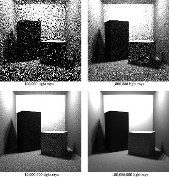
Images computed using light tracing using 100,000, 1,000,000, 10, 000, 000 and 100, 000, 000 light rays, respectively.
5.7.2 Light Tracing versus Ray Tracing
Stochastic light tracing and ray tracing are dual algorithms and, in theory, solve the same transport problem. The camera acts as a source of importance during light tracing, while the light sources are the source of radiance in stochastic ray tracing. Shadow rays and contribution rays are each other’s dual mechanism for optimizing the computations of final flux through a pixel.
Which algorithm performs better or is more efficient? It is generally accepted that stochastic ray tracing will perform better, but there are several factors that can contribute to the efficiency of one algorithm over the other:
Image size versus scene size. If the image only shows a very small part of the scene, it is to be expected that many particles shot from the light sources during light tracing will end up in parts of the scene that are only of marginal importance to the light transport relevant for the image. Stochastic ray tracing will perform better, because the radiance values to be computed are driven by the position of the camera and individual pixels, and so we can expect less work to be wasted on computing irrelevant transport paths.
Nature of the transport paths. The nature of transport paths also might favor one transport simulation method over the other. Shadow rays or contribution rays work best at diffuse surfaces, since the direction (towards the light sources or towards the camera) cannot be chosen. At a specular surface, there is a very high likelihood that those rays will yield a very small contribution to the final estimator. Thus, we would like to trace rays as much as possible over specular surfaces before we send out a shadow ray or contribution ray. This means that for mirrored images (where the light hits a diffuse surface before it hits a specular surface), we prefer ray tracing, and for caustics (where the light hits specular surfaces before diffuse surfaces), we would prefer light tracing. This principle is applied in building up caustic-maps with the photon-mapping algorithm [83].
Number of sources. In ray tracing, the sources for the transport we are simulating are the light sources; in light tracing, the importance sources are the individual pixels. This also has some effect on the efficiency of both algorithms, especially when sources are to be moved, in conjunction with an algorithm where partial information of the transport simulation is stored in the scene. It can be imagined that when a light-tracing algorithm is used, we could store all endpoints of all paths, and only retrace the contribution rays when the camera moves.2 This is not as easy with ray tracing. On the other hand, if we want to apply a similar scheme to ray tracing and a moving light source, it will not be straightforward, since the number of importance sources (or pixels) is much larger, and separate information needs to be stored for all of them.
In theory, ray tracing and light tracing are dual algorithms, but in practice, they are not equivalent, since we usually want to compute a final image and not an “importance image” for each of the light sources. Only in the latter case would the algorithms be really dual and equivalent.
5.7.3 Related Techniques and Optimizations
In global illumination literature, tracing rays starting at the light sources has been used in many different forms and with different names (particle tracing, photon tracing, backwards ray tracing, etc.), and has mostly been used as part of multipass algorithms, and not so much as an algorithm to compute images by itself.
In [23], light is distributed from light sources to immediate visible diffuse surfaces, which are then classified as secondary light sources. These new secondary light sources are then treated as regular light sources in the subsequent ray-tracing pass. Complex interactions associated with caustics have been computed using backwards beam tracing [225]. Beams, generated at the light sources, are reflected through the scene at specular surfaces only, and a caustic polygon is stored at diffuse surfaces. Later, the caustic polygon is taken into account when rendering pixels in which this caustic is visible.
Two-dimensional storage maps for storing light-traced information have also been proposed in various forms and in various algorithms. These maps also result from a light-tracing pass and are used to read out illumination information during a subsequent ray-tracing pass. Examples of two-dimensional storage maps can be found in [24] and [5].
Bidirectional ray tracing combines ray tracing and light tracing. When computing the radiance value for a pixel, both a path starting at a light source and a path starting at the eye are generated in the scene. By linking up their end- and midpoints, an estimator for the radiance is found. This technique is able to combine advantages of both light tracing and ray tracing, and each of those can actually be seen as a special case of bidirectional ray tracing.
The most successful applications of light tracing, however, are in the photon-mapping and density-estimation algorithms. A more complete discussion of some of these techniques is given in Chapter 7.
The light-tracing algorithm itself has also been optimized using adaptive sampling functions. Using several iterations of light, tracing passes, adaptive PDFs are constructed, such that particles are traced more efficiently towards the camera ([41], [42]).
5.8 Summary
This chapter outlined stochastic path tracing, one of the most commonly used algorithms to compute global illumination solutions to the rendering equation. By applying Monte Carlo integration schemes to the rendering equation, various stochastic path tracing algorithms can be developed, including simple stochastic ray tracing, optimizations through the use of shadow rays, various schemes for indirect illumination, etc. An interesting variant is stochastic light tracing, the dual algorithm of stochastic ray tracing, which traces rays from the light sources towards the eye. For more details on developing ray-tracing algorithms, Shirley’s book [170] is an excellent starting point.
5.9 Exercises
All exercises listed here require the rendering of various images using a ray tracer. When testing the various methods, it is usually a good idea to render the images at a low resolution. Only when one is fully convinced that the rendering computations are implemented correctly, images can be rendered at a high resolution, and the number of samples for each rendering component can gradually be increased.
- Implement a simple stochastic ray tracer that is able to render scenes with direct illumination only. The type of geometric primitives that are included is not important; it can be limited to triangles and spheres only. Surfaces should have a diffuse BRDF, and area light sources should be included as well. This simple ray tracer can serve as a skeleton ray tracer to use in subsequent exercises.
- Experiment with casting multiple shadow rays towards the light sources. Vary the number of samples per light source, as well as the sampling pattern (uniform, uniform stratified, etc.). Compare images with and without explicit light source sampling for computing the direct illumination. Independent of the sampling strategy used, the images should always converge to the same exact solution.
- Experiment with multiple viewing rays cast per pixel, in order to solve aliasing problems. Again, vary the number of rays, as well as the sampling pattern. Zoom in on an area of the image containing an object-object visual discontinuity and study the results.
- Include the Cook-Torrance shader from Chapter 3 in the skeleton ray tracer. The specular highlights should be visible especially on rounded objects such as spheres. Is the computation of the highlights affected by the sampling scheme used for direct illumination?
- Add the computation of indirect illumination to your skeleton ray tracer. This requires the implementation of a sampling scheme over the hemisphere of directions around a surface point. As before, experiment with various sampling schemes to examine the effect on the indirect illumination component. Also change the absorption value used in the Russian roulette termination scheme.
- Using the hemisphere sampling from the previous exercise, implement the direct illumination computation without explicitly sampling the light sources. Only when a random ray accidently reaches the light source, a contribution for the illumination of the pixel is found.
- Add the direct and indirect illumination components together to render the full global illumination solution of a given scene. Design a user interface such that all different sampling parameters can be adjusted by the user before the rendering computation starts.
1The terms ray tracing and path tracing are often used interchangeably in literature. Some prefer to use the term path tracing for a variant of ray tracing where rays do not split into multiple rays at surface points.
2This would be equivalent to a point-rendering of all end points of the light-paths.