
Chapter 4
Strategies for Computing Light Transport
4.1 Formulation of the Rendering Equation
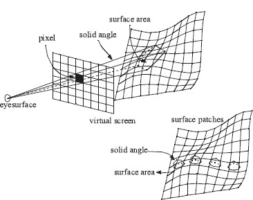
The global illumination problem is basically a transport problem. Energy emitted by light sources is transported by means of reflections and refractions in a three-dimensional environment. We are interested in the energy equilibrium of the illumination in the environment. Since the human eye is sensitive to radiance values, and since we want to compute photorealistic images, we are primarily interested in radiance values or average radiance values computed over certain areas and solid angles in the scene. The latter means that we should compute flux values for several areas of interest, which will be referred to as sets. The exact geometric shape of these sets can vary substantially, depending on the requested level of accuracy. As will be explained in subsequent chapters, ray tracing algorithms define sets as surface points visible through a pixel, with regard to the aperture of the eye. Radiosity algorithms often define sets as surface patches with the reflecting hemisphere as the directional component (Figure 4.1). Other algorithms might follow different approaches, but the common factor is always that for a number of finite surface elements and solid angle combinations, average radiance values need to be computed.
As explained in Chapter 2, the fundamental transport equation used to describe the global illumination problem is called the rendering equation and was first introduced into the field of computer graphics by Kajiya [85]. The rendering equation describes the transport of radiance through a three-dimensional environment. It is the integral equation formulation of the definition of the BRDF and adds the self-emittance of surface points at light sources as an initialization function. The self-emitted energy of light sources is necessary to provide the environment with some starting energy.
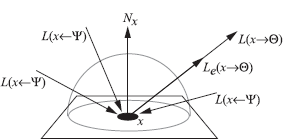
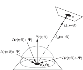
The radiance leaving some point x, in direction Θ, is written as:
L(x→Θ)=Le(x→Θ)+∫Ωxfr(x,Ψ↔Θ)L(x←Ψ)cos(Nx,Ψ)dωΨ. (4.1)
The rendering equation tells us that the exitant radiance emitted by a point x in a direction Θ equals the self-emitted exitant radiance at that point and in that direction, plus any incident radiance from the illuminating hemisphere that is reflected at x in direction Θ. This is illustrated in Figure 4.2.
Emission can result from various physical processes, e.g., heat or chemical reactions. The emission can also be time-dependent for a single surface point and direction, as is the case with phosphorescence. In the context of global illumination algorithms, one usually is not interested in the nature of the source of the self-emitted radiance of surfaces. Self-emitted radiance is merely considered as a function of position and direction.
As was shown in Chapter 2, it is possible to transform the rendering equation from an integral over the hemisphere to an integral over all surfaces in the scene. Both the hemispherical and area formulation contain exitant and incident radiance functions. We know that radiance remains unchanged along straight paths, so we can easily transform exitant radiance to incident radiance and vice-versa, thus obtaining new versions of the rendering equation that contain exitant or incident radiance only. By combining both options with a hemispheric or surface integration, we obtain four different formulations of the rendering equation.
The formulations that integrate over surfaces or hemispheres are all mathematically equivalent. However, there can be some important differences when one develops algorithms starting from a specific formulation. For completeness, we list all possible formulations of the rendering equation.
4.1.1 Exitant Radiance, Integration over the Hemisphere
The incident radiance in the classic form of the rendering equation is replaced by the equivalent exitant radiance at the nearest visible point y = r(x, Ψ), found by evaluating the ray-casting function (Figure 4.3):
L(x→Θ)=Le(x→Θ)+∫Ωxfr(x,Ψ↔Θ)L(y→−Ψ)cos(Nx,Ψ)dωΨ,
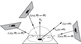
with y = r(x, Ψ). When designing an algorithm based on this formulation, one will integrate over the hemisphere, and as part of the function evaluation for each point in the integration domain, a ray will be cast and the nearest intersection point located.
4.1.2 Exitant Radiance, Integration over Surfaces
The hemispherical equation is transformed to an integral over all surface points (Figure 4.4):

L(x→Θ)=Le(x→Θ)+∫Afr(x,Ψ↔Θ)L(y→→yx)V(x,y)G(x,y)dAy,
with
G(x,y)=cos(Nx,Ψ)cos(Ny,−Ψ)r2xy.
The main difference with the previous formulation is that incident radiance at x is seen as originating at all surfaces in the scene and not only at the hemisphere Ωx. Algorithms using this formulation will need to check the visibility V (x, y), which is slightly different than casting a ray from x in a direction Θ.
4.1.3 Incident Radiance, Integration over the Hemisphere
In order to transform the hemispherical rendering equation to incident radiance values only, we again make use of the invariance of radiance along a straight path. However, we also have to write the initial self-emitted radiance Le as an incident measure. The concept of incident radiance Le may seem odd. It is relatively easy to imagine the incident radiance at a surface point, but it is harder to imagine the incident Le function corresponding to a certain light source (Figure 4.5).
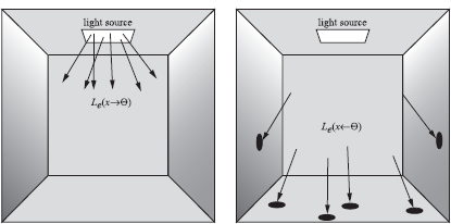
Exitant surface radiance for a light source at the ceiling and corresponding incident surface radiance.
We obtain the following equation:
L(x←Θ)=Le(x←Θ)+∫Ωyfr(y, Ψ↔–Θ)L(y←Ψ) cos(Ny, Ψ)dωΨ,
with y = r(x, Θ). This equation is graphically represented in Figure 4.6.
4.1.4 Incident Radiance, Integration over Surfaces
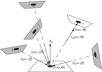
Following a similar procedure for incident radiance from surfaces, we get the following equation (Figure 4.7):
L(x←Θ)=Le(x←Θ)+∫Afr(y,Ψ↔→yz)L(y←→yz)V(y,z)G(y,z)dAz,
with y = r(x, Θ).
4.1.5 Radiant Flux
The ideal solution to the global illumination problem would consist of finding all values of the radiance function for all possible (surface) points and all directions relative to those points. It is easy to see that this is not possible in practice. This would require the computation of (discrete) function values over all points belonging to a piecewise-continuous four-dimensional set in the five-dimensional space.
Most global illumination algorithms are, therefore, aimed at computing the average radiance over some chosen sets of points and directions. One possible way of computing the average radiance value over a set is to compute the radiant flux over that set. By assuming the radiance to be changing slowly over the set, an average radiance value can be obtained by dividing the flux by the total area and total solid angle of the set. Ray tracing algorithms use this technique by computing the flux through a pixel with regard to the aperture of the eye. Radiosity algorithms typically compute the flux, leaving a surface element or patch over the entire hemisphere.
The radiant flux can be expressed in terms of radiance by integrating the radiance distribution over all possible surface points and directions around these surface points belonging to the set for which the flux has to be computed. Let S = As × Ωs denote the set of surface points As and directions Ωs we are interested in. Then the flux Φ(S) leaving S can be written using the measurement equation (see Chapter 2),
Φ(S)=∫As∫ΩsL(x→Θ)cos(Nx,Θ)dωΘdAx.
By introducing the initial importance function We(x ← Θ), we can rewrite the above integral by integrating over all surfaces A in the scene, and by integrating over the complete hemisphere Ω for all surface points:
Φ(S)=∫A∫ΩL(x→Θ) We(x←Θ) cos(Nx, Θ)dωΘ dAx, (4.2)
with
We(x←Θ)={1if (x, Θ)∈S0if (x, Θ)∈S.
The average radiance value associated with the set is then expressed by
Laverage=∫A∫ΩL(x→Θ) We(x←Θ) cos(Nx, Θ) dωΘ dAx∫A∫ΩWe(x←Θ) cos(Nx, Θ) dωΘdAx.
Depending on the geometry of the set S, the denominator of this fraction can sometimes be computed analytically.
The global illumination problem can, therefore, be specified as computing the radiant fluxes for a certain number of well-defined sets. These sets are usually continuous and belong to the space A × Ω. The fluxes are computed by evaluating Equation 4.2. The integrand contains the radiance function L, which needs to be evaluated using one of four possible recursive Fredholm equations. Solving the Fredholm equations requires numerical algorithms, which are the focus of many global illumination algorithms, and which will be treated in more detail in Chapter 5 and Chapter 6.
4.2 The Importance Function
4.2.1 Definition
So far, we have thought of the global illumination problem as computing the incident or exitant radiance at a point x and in a direction Θ, given a specific distribution of light sources. Thus, a certain function Le, defined over all points and directions belonging to A × Ω, determines a function L, also defined over A × Ω, by means of radiance transport. The relation between Le and L is given by the rendering equation. This section looks in more detail at the importance function, which will define an adjoint transport quantity. We will first look at the importance function in an intuitive manner, and afterwards we will deal with some more complex mathematical issues. The importance function was first introduced in computer graphics by Pattanaik [139]. Some authors prefer to use the term potential function, but this function is equivalent to the importance function described here.
Suppose we are interested in the flux Φ(S) leaving a set S, consisting of points and directions around those points. Instead of starting from a fixed Le distribution, we want to compute the possible influence of each pair (x, Θ) on Φ(S). To put it more precisely: if a single radiance value (a light source covering a differential surface area and differential solid angle) L(x → Θ) is placed at (x, Θ), and if there are no other sources of illumination present, how large is the resulting value of Φ(S)? The weight we have to attribute to L(x → Θ) in order to obtain Φ(S) is called the importance of (x, Θ) with regard to S and is written as W(x ← Θ).
The importance value does not depend on the exact magnitude of L(x → Θ), since any resulting flux scales linearly due to the linearity of a BRDF with regard to reflection of incident radiance. This is true regardless of the number of possible light paths between (x, Θ) and S, and regardless of the number of reflections. Thus, W(x ← Θ) depends only on the geometry of the scene and the reflective properties of the materials.
The next step is to derive an expression or equation that describes the importance W(x ← Θ). This expression can be written down by considering two ways in which contributions from the flux resulting from L(x → Θ) can be made to Φ(S):
Self-contribution. If (x, Θ) ∈ S, then L(x → Θ) fully contributes to Φ(S). This is called the self-importance of the set S and is written as We(x ← Θ) (see also Equation 4.2):
We(x←Θ)={1if (x, Θ)∈S0if (x, Θ)∈S.
Contribution through one or more reflections. We also have to consider all indirect contributions to the resulting flux. It is possible that some part of L(x → Θ) contributes to Φ(S) through one or more reflections at several surfaces. We know that the radiance L(x → Θ) travels along a straight path and reaches a surface point r(x, Θ). The energy is reflected at this surface point according to a hemispherical distribution determined by the BRDF. Thus, we have a hemisphere of directions at r(x,Θ), each emitting a differential radiance value as a result of the reflection of the radiance L(r(x, Θ) ← –Θ). By integrating the importance values for all these new directions, we have a new term for W(x ← Θ). By taking into account the reflection, and thus the BRDF values, we obtain the following equation for both terms combined:
W(x←Θ)=We(x←Θ)+ ∫Ωzfr(z, Ψ↔– Θ) W(z←Ψ) cos(Nr(x, Θ), Ψ)dωΨ, (4.3)
with z = r(x, Θ).
4.2.2 Incident and Exitant Importance
Mathematically, Equation 4.3 is identical to the transport equation of incident radiance. It is, therefore, appropriate to associate the notion of “incidence” also to importance, since importance as a transport quantity behaves in exactly the same way as an incident radiance.
The source function We depends on the nature of the set S. If one wants to compute individual flux values for pixels, We(x ← Θ) = 1 if x is visible through the pixel and Θ is a direction pointing through the pixel to the aperture of the virtual camera. For a radiosity algorithm, S probably is a single patch and for each surface point, the full hemisphere of directions.
To further enhance the analogy, we can also introduce exitant importance by formally defining W(x → Θ):
W(x→Θ)=W(r(x,Θ)←−Θ).
This definition implies that we attribute the property of invariability along straight lines also to importance, which is in accordance with the definitions of radiance and importance. It is then easy to prove that exitant importance has exactly the same transport equation as exitant radiance:
W(x→Θ)=We(x→Θ)+∫Ωxfr(x,Ψ↔Θ)W(x←Ψ)cos(Nx,Ψ)dωΨ.
As incident self-emitted radiance is not very intuitive to think about, so is self-emitted exitant surface importance. In the case of small sets with a narrow solid angle domain, self-emitted importance is sometimes easier to visualize by introducing a light detector. Such a detector has no influence on the propagation of light energy through the scene but detects only the flux of the set in question. Self-emitted exitant importance can then be thought of as emanating from this hypothetical detector, which acts as a source of importance. The concept of light detectors works extremely well when applied to an image generation algorithm, such as ray tracing. The eye point can then be considered as the source of exitant importance, directed towards the different pixels.
4.2.3 Flux
An expression for the flux of a set based on the importance function can now be deduced. The light sources are the only points that provide light energy in an environment. Their radiance values account for the illumination of the whole scene. Only the importance values of these points need to be considered when computing the flux. Given a certain set S,
Φ(S)=∫A∫ΩxLe(x→Θ)W(x←Θ)cos(Nx,Θ)dωΘdAx.
We can integrate over all surface points A, since Le is suitably defined to be 0 at points and directions not belonging to light sources. This equation, together with the transport equation of the importance function, provides us with an alternative way of solving the global illumination problem.
It is also possible to write Φ(S) in the form
Φ(S)=∫A∫ΩxLe(x←Θ)W(x→Θ)cos(Nx,Θ)dωΘdAx,
and also
Φ(S)=∫A∫ΩxL(x→Θ)We(x←Θ)cos(Nx,Θ)dωΘdAx,
Φ(S)=∫A∫ΩxL(x←Θ)We(x→Θ)cos(Nx,Θ)dωΘdAx.
Thus, the flux of a given set can be computed by four different integral expressions, and each can be computed through double integration over all surfaces or hemispheres.
We now have two different approaches to solve the global illumination problem. The first approach starts from the definition of the set and requires the computation of the radiance values for the points and directions belonging to that set. The radiance values are computed by solving one of the transport equations describing radiance. So, we start from the set, working towards the light sources by following the recursive transport equation.
The second approach computes the flux of a given set by starting from the light sources and computes for each light source the corresponding importance value with regard to the set. The importance value also requires the use of one of the recursive integral equations. This kind of algorithm starts from the light sources and works towards the set by following the recursive transport equation for importance.
4.3 Adjoint Equations
The previous section described transport equations for incident and exitant radiance, incident and exitant importance, and also gave four different expressions for the flux. Moreover, we have a choice of integrating over a hemisphere or over all possible surfaces in the scene. This section will point out the symmetry between the two approaches more clearly. We will often refer to the complete radiance or importance functions, defined over A × Ω. We will denote them by L, L→ (exitant radiance), L← (incident radiance), W, W→ (exitant importance), or W← (incident importance) where appropriate.
4.3.1 Linear Transport Operators
The recursive integral equations that describe transport of radiance and importance can be written in a more concise form, using linear operators. The reflectance part of the rendering equation can actually be considered as an operator that transforms a certain radiance distribution over all surface points and directions to another distribution that gives us the reflected radiance values after one reflection. This new distribution is again a function of radiance values defined over the whole scene. We denote this operator by ?. ?L is a new function, also defined over A × Ω.
L(x→Θ)=Le(x→Θ)+T L(x→Θ);T L(x→Θ)=∫Ωxfr(x, Ψ↔Θ)L(r(x, Θ)→–Ψ) cos(Nx, Ψ)dωΨ.
The same operator can also be written using the area integral formulation, since it is just a different parameterization.
In an analogous manner, the transport equation for the incident importance function W← can also be described by use of a transport operator, which we denote by ?:
W(x←Θ)=We(x←Θ)+QW(x←Θ);QW(x←Θ)= ∫Ωr(x,Θ) f(r(x,Θ),Ψ↔−Θ)W(r(x,Θ)←Ψ). cos(Nr(x,Θ),Ψ)dωΨ.
or the equivalent expression using area integration.
Since L← and W→ are described with the same transport equations as W← and L→, respectively, we have four transport equations to describe radiance and importance transport in a three-dimensional environment:
L→=L→e+?L→;W←=W←e+QW←;L←=L←e+QL←;W→=W→e+?W→.
These four equations clearly illustrate the symmetry between radiance and importance distributions.
4.3.2 Inner Product of Functions
In the function space defined over the five-dimensional domain A × Ω, it is possible to define an inner product of an exitant function F→ and an incident function G← as
〈F→,G←〉=∫A∫ΩF(x→Θ)G(x←Θ)cos(Nx,Θ)dωΘdAx.
The same inner product can be written using area integration, and introducing the visibility function into the equation:
〈F→,G←〉=∫A∫AF(x→→xy)G(x←→xy)G(x,y)V(x,y)dAxdAy.
The flux of a set S can now be seen as an inner product of a radiance function and an importance function. Based on previous transport equations, we have four different expressions available to write the flux as an inner product:
Φ(S)=〈L→,We←〉;Φ(S)=〈Le→,W←〉;Φ(S)=〈L←,We→〉;Φ(S)=〈Le←,W→〉.
4.3.3 Adjoint Operators
Two operators, ?1 and ?2, operating on elements of the same vector-space V, are said to be adjoint with respect to an inner product 〈F, G〉 if
∀F,G∈V:〈?1F,G〉=〈F,?2G〉.
?2 is called the adjoint operator of ?1 and is written as ?*1.
By manipulating the area integral formulation, one can prove that the above defined operators ? and ?, which describe transport of radiance and importance, are adjoint to each other for the above defined inner product describing the flux Φ(S), or ?* = ?, and thus
L←=L←e+?*L← and W←=W←e+?*W←.
Due to this property of adjointness, the equivalence of the different expressions for the flux of a given set S can be written in a very compact notation. For example, the flux expressions using exitant radiance and incident importance can be transformed into each other using the properties of an inner product and the adjointness of the transport operators:
Φ(S)=〈L→,We←〉=〈L→,W←−T*W←〉=〈L→,W←〉−〈L→,?*W←〉=〈L→,W←〉−〈?L→,W←〉=〈L→−?L→,W←〉=〈Le→,W←〉.
The equations describing the global illumination problem, which give expressions for the flux and transport equations for radiance or importance, can thus be written in several different ways. The different choices to make are:
- Using incident or exitant functions for radiance and importance.
- Using importance-based or radiance-based transport equations.
- Integration over hemispheres or surface area integration.
We have, therefore, four possible, mathematically equivalent formulations of the global illumination problem:
Φ(S)=〈L→, W←e〉Φ(S)=〈L→e, W←〉L→=L→e+T L→;W←=W←e+T*W←;(4.4)Φ(S)=〈L←, W→e〉Φ(S)=〈L←e, W→〉L←=L←e+T*L←;W→=W→e+T W→.
Similar descriptions for the global illumination problem, using incident and exitant functions, and operators that act in function space, have been presented by other authors [25], [26], [204]. Some of these authors introduce additional operators, such as the geometry operator, which transforms an incident function into the corresponding exitant function (or vice-versa), by making use of the invariability along straight paths. The inner product can also be defined differently, not including the cosine term. However, we feel that the symmetry in this case is not as clear as it is presented here.
4.4 Global Reflectance Distribution Function
4.4.1 Description
Given the transport equation of L→, it is obvious that each single radiance value in the scene is dependent on the initial distribution given by Le→. For the flux of a complete set, such dependency is expressed by the importance function W←. We will now introduce a function that expresses the relation between a single L(x → Θ) value at an arbitrary chosen point, and the initial Le→ distribution. Such relation already exists as the transport equation for radiance. However, we want to derive a more direct function, instead of a recursive formulation. We will call this function the global reflectance distribution function [102, 41], or GRDF.
The GRDF is a four-dimensional transfer function that describes the entire light transport in a three-dimensional scene between two pairs (x, Θ) and (y, Ψ). It has the characteristics of both an incident and an exitant function, since the transfer can happen in both directions. We will write the GRDF as Gr(x ← Θ, y → Ψ).
Intuitively, the Gr(x ← Θ, y → Ψ) describes some sort of global transport between two point-direction pairs and can be thought of as the contribution one pair makes, if it would act as a differential source of transport quantity, to the transport quantity measured at the other pair. In other words, we want the GRDF to be such that
L(y→Ψ)=∫A∫ΩxLe(x→Θ)Gr(x←Θ,y→Ψ)cos(Nx,Θ)dωΘdAx. (4.5)
So, Gr(x ← Θ, y → Ψ) expresses the influence of the total power leaving dAx through a solid angle dωΘ on the final value of the radiance measured at y in direction Ψ, through any number of reflections on intermediate surfaces. The GRDF can thus be considered as some kind of response function in the three-dimensional environment. In mathematical physics, a function like the GRDF is usually called the Green’s function of a problem.
Since the transport is reciprocal, we want a similar equation for the importance:
Similar equations hold for incident radiance and exitant importance.
Differentiating the above equations yields
and
This is very similar to the definition of the common BRDF, which describes a similar property for exitant radiance and incident irradiance at a single surface point. The GRDF extends this concept and describes the relationship between any two radiance or importance values, taking into account all possible reflections in the scene. The BRDF can be considered as a special case of the GRDF. The name global reflectance distribution function is therefore quite appropriate.
4.4.2 Properties of the GRDF
Transport Equations
The following adjoint transport equations both describe the behavior of the GRDF:
with δ(x ← Θ, y → Ψ) being a proper Dirac impulse defined in the four-dimensional domain. When using the ? and ?* operators, we have to keep in mind that ? operates on the exitant part of Gr, and that ?* operates on the incident part of Gr.
Transforming Arguments
Another useful property of Gr is that the arguments can be switched, in much the same manner as the directions of the BRDF can be reversed:
This relationship is the generalization of the property of the BRDF, by which the incident and exitant directions can switch roles, resulting in the same BRDF value.
Flux
It is now possible to write an expression for the flux Φ(S) using the GRDF. This expression follows from integrating Equation 4.5 and Equation 4.6:
4.4.3 Significance of the GRDF
The GRDF allows us to describe the global illumination problem in a very short and elegant format, independent of any initial distributions for self-emitted radiance or importance. The GRDF is only dependent on the geometry of the scene and the reflective properties of the surfaces. No positioning of light sources is assumed, nor is it assumed that we know where we will place the sources of importance for which flux values need to be computed.
Consequently, if the GRDF would be known, it is possible to compute various fluxes for a number of light sources and importance distributions. It suffices to evaluate Equation 4.7, which is a nonrecursive integral. In practice, however, this may be difficult to achieve, since the GRDF has as arguments two positions and two directions. If one wants to compute and store the GRDF for a significant number of arguments, or if we want to compute a discretized version of the GRDF, the required amount of memory can easily become huge.
A Monte Carlo algorithm based on the computation of the GRDF, so-called bi-directional path tracing, is discussed in Chapter 7.
4.5 Classification of Global Illumination Algorithms
In the previous section, it was shown that there are four possible expressions for the flux of any given set of surface points and directions in a global illumination environment.
When designing a global illumination algorithm, which means we want to compute fluxes for specific sets in the scene, we can choose whether we want to use incident radiance combined with exitant importance in the algorithm, or exitant radiance combined with incident importance. Furthermore, we can choose to consider radiance or importance as the transport quantity which has to be computed by solving a recursive integral transport equation. This implies there are four different classes of algorithms trying to compute global illumination solutions.
4.5.1 Incident and Exitant Representations
A first option to consider is whether we want to represent radiance as an exitant or incident measure (which automatically determines importance to be incident or exitant, respectively). From a mathematical point of view, the incident and exitant functions can be transformed into each other because they remain invariant along straight lines. But the choice is important with regard to representation of the functions and storage requirements.
The previous section showed that it is easier to intuitively reason about exitant radiance and incident importance. The initial incident radiance distribution due to a light source equals zero at the surface points belonging to that light source but has a value different from zero at surface points directly visible to that light source. All points and directions belonging to a set for which we want to compute the flux have an initial incident importance value different from zero. Exitant importance is only different from zero in points that are visible to the set in question. Thus, it is a lot more convenient to think in terms of exitant radiance and incident importance.
A second issue to be considered is the nature of the incident and exitant functions with regard to continuity over the integration domains. Finite element methods make certain assumptions about the shape of the functions under consideration in order to achieve a required precision. It is, therefore, important to know whether or not features such as discontinuities are present in the function we want to compute. All of the transport quantities described above, incident and exitant, can have discontinuities in the surface area domain. It suffices to think of shadow boundaries or material boundaries for exitant radiance or directly versus indirectly lit areas for incident radiance. Analogous phenomena are present in the importance function. However, there is a difference when considering these functions in the directional domain. If the BRDF itself is a continuous function (which might not always be the case, e.g., ideal specular surfaces), then exitant radiance is continuous over the hemisphere. Incident radiance can have discontinuities, due to the angle under which light sources light a surface. The same can be said about the importance function: incident importance can have discontinuities in the directional domain, but exitant importance is continuous.
Whatever option we choose, we always have to work with a pair of functions consisting of an exitant and an incident one, so we will always have a function that has at least discontinuities in the directional domain. However, the discontinuities only matter if we construct an algorithm that uses a data representation not well suited to represent these kinds of discontinuities. For instance, in [173], spherical harmonic functions are used to represent directional distributions. They are not capable of reproducing discontinuities accurately, so it may be a bad choice to work with a combination of incident radiance and spherical harmonic functions. If we want to somehow represent discontinuities in the spatial domain, they should be integrated in the structure of the finite elements. This technique is known as discontinuity meshing [71], [111], [112].
4.5.2 Series Expansion
Once we have chosen a pair of an exitant and an incident function, the next choice to make is what transport equation to use; or more precisely what measure will we consider to be unknown with regard to the given set, and thus needs to be computed using an appropriate recursive integral equation? For this computation, we have the following data available:
- A specific initial radiance distribution Le→, thereby defining all the light sources present in the environment.
- A specific initial importance distribution We←, thereby defining the set S for which we want to compute a flux. A typical situation might be that we want to compute flux values for all areas visible through each pixel (and thus each pixel defines its own set S).
- A given scene description, thereby defining the geometric kernel function G(x,y), the visibility function V(x,y), and the material properties or BRDFs of all surfaces in the scene.
From a mathematical point of view, we have two different expressions, given by two inner products, from which we can start the computation for any Φ(S). We can start from the initial radiance distribution Le→ and compute W← by evaluating its transport equation, or we can start from the initial importance distribution We← and compute L→ The first step of the computation, no matter which inner product we choose as a starting point, is the substitution of the unknown function by its appropriate transport equation. For example, if we start from 〈Le→, W←〉, we can write down the following expansion of the inner product:
This first substitution gives us a first approximate term 〈Le→, We←〉 (which only contains known terms) of the final solution. The second term needs to be expanded further:
This provides us with a second term to compute. However, we could also obtain an expression for the second term in another way, by using the property of adjoint operators. By shifting ?* in the inner product, we can express Φ(S) as
Mathematically, the second and third terms of Equation 4.8 are, of course, equal to the second and third terms of Equation 4.9 (due to adjointness of ? and ?*). By further expanding the series and by using the same adjoint property, we are able to write Φ(S) in many different ways. Indeed, we have the option of using the adjoint property in any step of the expansion. All possibilities can be represented by a binary tree of possible expansions, originating from (Le→, We←):
Exactly the same tree can be constructed by expanding 〈L→, We←) and by using the same kind of substitutions. The computation of a single flux can therefore be thought of as the sum of several inner products. For each inner product, we have a choice of functions to multiply with each other, and which are equivalent to each other due to the duality of the transport operator.
4.5.3 Physical Interpretation
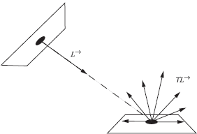
The above series of inner products has, of course, a corresponding physical meaning. In order to better grasp this physical meaning, it is important to have a look at what the functional operators ? and ?* actually do in a three-dimensional environment. Operator ?, operating on an exitant function, was defined as
The operator ? transforms a function L→ int another function ?L→. ?L→ is the function we obtain when we “propagate” L→ in the environment according to the rules of the transport equation defining ?. Thus, ?L→ is the result of propagating L→, and evaluating this propagation in (x, Θ). The operator ? not only implies propagating radiance along its straight path of traversal but also implies reflecting it once on a surface, in order to obtain another exitant function at the reflection point. Figure 4.8 illustrates this for a function L→ that exists only in a single point and a single direction.
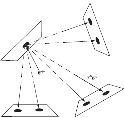
?*, the adjoint operator of ?, was defined as
The operator ?* behaves in a similar way as ? but propagates incident functions through one reflection on the point on which they are incident. This is illustrated in Figure 4.9.
One might be tempted to use the terms “shooting” and “gathering” to denote these operations. The operator ? may be thought of as a shooting operation, because ?L→ seems to be the resulting function when we “shoot” L→ forward. However, the terms shooting and gathering are usually applied to the way algorithms work and not to mathematical operations. It might be more convenient to think in terms of propagating the function. Whether the function is of an incident or exitant nature determines what operator (? or ?*) has to be used for the propagation.
If we look at the series of inner products that composes Φ(S), we can see that it is a succession of ? and ?* operations applied to the initial radiance and importance distributions. For example, the second term in the expansion, which expresses direct illumination, can be computed by propagating We← or by propagating Le→. By successively repeating these steps, we gradually build up the flux Φ(S). At each step during the evaluation, we have a choice of evaluating the next term by applying a ? or ?* operation on one of the intermediate resulting functions. For example, we might propagate the radiance distribution twice, then propagate the importance function once, propagate the radiance again, etc.
The following figures illustrate this by means of a simple example. A simple scene consisting of three surfaces is depicted in Figure 4.10. For simplicity, let us also assume that there are only three directions per surface, and that functions are only defined in one surface point. The surface labeled a is a light source, emitting radiance only in the direction of surface d (exitant radiance from surface to surface is represented by a single arrow, instead of a complete directional distribution, in order not to overly complicate the figure). Propagating this initial radiance distribution by applying operator ? once results in a new distribution shown in Situation 2. Indeed, the self-emitted radiance from surface a reaches surface d, where it is reflected over the entire hemisphere (just three directions in this example), and thus emits radiance toward surfaces a, b, and c. One more propagation is shown in Situation 3. Surfaces a, b, and c emit radiance toward all other surfaces. All further propagations would result in all four surfaces emitting radiance toward all other surfaces, although the exact numerical values vary for each propagation (dependent on the values of the local BRDF, and due to absorption, each further propagation carries less total power).
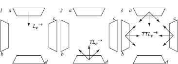
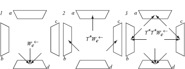
Figure 4.11 shows the various propagations for the importance function by applying operator ?*. Suppose we want to compute the flux leaving surface d. The corresponding distribution is shown in Situation 1. We→ is defined for all surface points belonging to d, and for all directions towards other surfaces. Applying the transport operator gives the results as shown in Situations 2 and 3. Further propagations result in all surfaces and all directions having an incident importance value attributed to them. As explained before, due to absorption and BRDF values, the exact numerical values would differ for each propagation.
In order to compute the flux, we now have to compute the various inner products, the summation of which provides us with a numerical value for the flux. This is represented in Figure 4.12. The top row shows the various propagations for the radiance distribution; the leftmost column gives the importance propagations. For each entry in the table, a thick line indicates at what surface points and for what directions a contribution to the inner product exists. Only if there are point-directions pairs that have a nonzero value for both propagations of L→e and We← is a contribution to the inner product found.
As such, we see that the contribution to the flux due to self-emittance equals 0, which is, of course, a quite logical result, since the importance-source and radiance-source do not overlap. In order to compute the contributions as a result of direct lighting (light that reaches the set unhindered
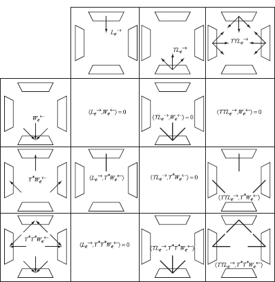
Successive propagations of exitant radiance and initial importance are shown in the top row and leftmost column, respectively. The entries in the table represent where nonzero values for the inner products can be found.
and contributes to the flux leaving that surface), we have the choice of propagating Le→, and thus computing 〈?Le→, We←〉, or propagating We← and thereby computing 〈Le→, ?*We←). Both inner products are equal, although the integration domain where the inner product is nonzero is different in both situations.
The next propagations compute the contributions to the flux through one or more reflections on intermediate surfaces. In this example, there are no contributions due to one intermediate reflection, but there is a contribution when the radiance is reflected at two surfaces.
The different choices available for expanding into a series of inner products are not mutually exclusive. Since all inner products at the same level of the expansion are mathematically and numerically equivalent, it is possible to compute them all and make a selection of one to use in the final result. This selection might be based on an error metric or on any other criteria that seem plausible. It also means that different terms can be combined in order to produce a possibly better result. For example, one might compute weighted averages, with the weight based on the relative reliability of the numerical results. The resulting expression will then, hopefully, be more correct than each inner product individually.
4.5.4 Taxonomy
Depending on what inner products are used, and how the propagation is being carried out, it is possible to make a taxonomy of different global illumination algorithms. A complete classification would lead us too far and is also partly covered in subsequent chapters. Detailed descriptions of the algorithms mentioned below are also covered in the next chapters.
- The traditional ray-tracing algorithm typically exploits the propagation of importance, with the surface area visible through each pixel being the source of importance. In a typical implementation, the importance is never explicitly computed, but by tracing rays through the scene and picking up illumination values from the light sources, it is done implicitly.
- Light tracing is the dual algorithm of ray tracing. It propagates radiance from the light sources and computes final inner products at the surfaces visible through each pixel.
- Bidirectional ray tracing propagates both transport quantities at the same time and, in its most advanced form, computes a weighted average of all possible inner products at all possible interactions.
- The equivalent algorithms in a radiosity context are, respectively, Gauss-Seidel radiosity progressive radiosity and bidirectional radiosity.
4.6 Path Formulation
The above derivation and classification of global illumination transport algorithms is based on the notion of radiance and importance. Also, the global reflection distribution function expresses the global transport between two point-direction pairs in the scene. Computing the fluxes can then be seen as computing an integral over all possible pairs of point-direction couples, evaluating the GRDF and the initial radiance and importance values. The GRDF itself is given by a recursive integral equation. By recursively evaluating the GRDF, all possible paths of different lengths in the scene are constructed.
One can also express global transport by considering path-space and computing a transport measure over each individual path. Path-space itself encompasses all possible paths of any length. Integrating a transport measure in path-space then involves generating the correct paths (e.g., random paths can be generated using an appropriate Monte Carlo sampling procedure) and evaluating the throughput of energy over each generated path. This view was developed by Spanier and Gelbard [183] and introduced into rendering by Veach [204]. The equation for the path formulation is
in which Ω* is the path-space, x̅ is a path of any length, and dµ(x̅) is a measure in path space. f(x̅) describes the throughput of energy and is a succession of G(x,y), V(x,y), and BRDF evaluations, together with a Le and We evaluation at the beginning and end of the path.
An advantage of the path formulation is that paths are now considered to be the sample points for any integration procedure. Algorithms such as Metropolis light transport or bidirectional ray tracing are often better described using the path formulation.
4.7 Summary
In this chapter, we defined a mathematical framework for describing the light transport equations and the global illumination problem. This mathematical framework encompasses two sets of dual equations.
On the one hand, the radiance transport equation is based on the notion of gathering radiance values at a surface point. It assumes that the light sources are fixed and that we have several sets of interest for which we want to compute a flux. Precomputing a solution based on radiance transport and storing it in the scene would allow us to generate various images, from different camera positions.
On the other hand, the importance transport equation expresses the influence of a surface point and associated direction, if it would be a light source on the illumination of a given set. It assumes the light sources can vary, but the set of interest remains fixed. Thus, if the camera would act as a source of importance, and if an importance solution is stored in the scene, it would be possible to change the nature and characteristics of the light sources.
Both transport equations are written as recursive integral equations, known as Fredholm equations of the second kind.
Both the transport of radiance and importance can be combined by introducing the global reflectance distribution function. The GRDF describes a general transfer property from one point-direction pair in the scene to another point-direction pair. As such, it can be considered as the core function for the global illumination problem.
Computing solutions for the transport equations can be done in various ways. It is possible to distribute radiance from the light sources into the scene, and collect it at the sets for which we want to compute a flux. Or, importance can be distributed from the importance sources and collected at the light sources, upon which we would know the flux for the importance source. We can also distribute both transport quantities at once and compute their interaction at the surfaces and directions at which they meet. Based on this notion, a taxonomy of various global illumination algorithms can be constructed.
4.8 Exercises
- Study the original formulation of the rendering equation as introduced by Kajiya [85]. It is different from the radiance formulation as mostly used today. Explain the differences. Could these differences have an influence on the final algorithms?
- Once you have studied Chapter 5 and Chapter 6, construct a taxonomy of global illumination algorithms. Look for similarities rather than differences. Is it important whether you render pixels (as in most path-tracing variants) or patches (as in most radiosity-based algorithms)?