3

Developing System Architectures

Recipes in this chapter

• Architectural trade studies
• Architectural merge
• Pattern-driven architecture
• Subsystem and component architecture
• Architectural allocation
• Creating subsystem interfaces from use case scenarios
• Specializing a reference architecture

System analysis pays attention to the required properties of a system (such as its functionality), while system design focuses on how to implement a system that implements those needs effectively. Many different designs that can realize the same functionality; system engineers must select from among the possible designs based on how well they optimize crucial system properties. The degree of optimization is determined by examining with Measures of Effectiveness (MoE) applied to the design. Design is all about optimization, and architecture is no different. Architecture is the integration of high-level design concerns that organize and orchestrate the overall structure and behavior of the system.

Design exists at (at least) three levels of abstraction. The highest level – the focus of this chapter – is architectural design. Architectural design makes choices that optimize the overall system properties at a system-wide level. The next step down, known as collaboration design, seeks to optimize collaborations of small design elements that collectively perform important system behaviors. Collaborative design is generally an order of magnitude smaller in scope than architectural design. Finally, detailed design individually optimizes those small design elements in terms of their structure or behavior.

Five critical views of architecture

The Harmony process defines six critical views of architecture, as shown in Figure 3.1. Each view focuses on a different aspect of the largest scale optimization concerns of the system:

• Subsystem/Component Architecture is about the identification of subsystems, the allocation of responsibilities to the subsystems, and the specification of their interfaces.
• Distribution Architecture selects the means by which distributed parts of the system nteract, including middleware and communication protocols; this includes, but is not limited to, network architecture.
• Concurrency and Resource Architecture details the set of concurrency regions (threads and processes), how semantic elements map into those concurrency regions, how they are scheduled, and how they effectively share and manage shared resources.
• Data Architecture focuses on how data is managed. It includes technical means and policies for data storage, backup, retrieval, and synchronization, as well as the overall data schema itself. Beyond that, this view includes the policies for ensuring data correctness and availability.
• Dependability Architecture refers to large-scale design decisions that govern the ability of stakeholders to depend on the system. This is subdivided into the Four Pillars of Dependability:
  • Safety Architecture – the large-scale mechanisms by which the system ensures the risk of harm is acceptable
  • Reliability Architecture – the system-wide decisions that manage the availability of services
  • Security Architecture – the important design decisions that control how the system avoids, identifies, and manages attacks
  • Privacy Architecture – how the system protects information from spillage
• Deployment architecture is the allocation of responsibilities to different engineering facets, such as software, electronics, and mechanical design concerns.

This chapter focuses on the development and verification of systems architecture with some key recipes, including the following:

• Selecting from architectural alternatives with trade studies
• Merging different use cases analyses together into a system architecture
• Application of architectural design patterns
• Creating the subsystem and component architecture
• Allocation of system properties into the subsystem architecture
• Defining system interfaces

Figure 3.1: Six critical views of architecture

General architectural guidelines

As previously shown in Figure 1.27, good architecture:

• Is architected early
• Evolves frequently
• Is as simple as possible (but no simpler than that)
• Is based on patterns
• Integrates into project planning via Technical Work Items
• Optimizes important system properties
• Is written down (specifically, modeled)
• Is kept current

The Architecture 0 recipe in Chapter 1, Basics of Agile Systems Modeling, concentrated on creating an early model of architecture so that more detailed engineering work had a structural context and to establish the feasibility of desired system capabilities early. Remember – from Chapter 1 – in the context of an agile approach, engineers establish an architectural roadmap in which architectural features that meet requirements are added incrementally over time. The recipes in this chapter will therefore be performed multiple times during the development of a product. Thus, the expectation is that architecture evolves throughout the development work as more functionality is added to the evolving system design.

This chapter provides some important recipes for architectural definition, whether it is done as Big-Design-Up-Front or in an incremental agile process.

Architectural trade studies

Trade studies are specifically concerned with the merit-based selection of approach or technology based on important concerns specific to the system development, system environment, or stakeholder needs. At a very fundamental level, trade studies are about making design choices to optimize important properties of the system at the expense of properties deemed less critical. To effectively perform trade studies, it is important to identify the things that can be optimized, the aspects subject to optimization, the MoE, and a set of alternatives to be evaluated.

Purpose

The purpose of performing an architectural trade study is to select an optimal design solution from a set of alternatives.

Inputs and preconditions

The inputs to this recipe are:

1. Functionality of concern, scoped as a set of requirements and/or use cases
2. Design options capable of achieving that functionality

Outputs and postconditions

The primary output of this recipe is an evaluation of alternatives, generally with a single technical selection identified as the recommended solution. This output is often formatted as a Decision Analysis Matrix. This matrix is normally formatted something like Table 3.1:

Candidate Solutions	Solution Criteria										Weighted Total
	Power Consumption (W1= 0.3)		Recurring Cost (W2 = 0.2)		Robustness (W3 = 0.15)		Development Cost (W4 = 0.1		Security W5 = 0.25)
	MoE	Score	MoE	Score	MoE	Score	MoE	Score	MoE	Score
Gigabit Ethernet Bus	2	0.6	2.7	0.54	4	0.6	8	0.8	4	1.0	3.54
1553 Bus	3	0.9	4	0.8	10	1.5	1.5	0.15	6	1.5	4.85
CAN Bus	6	1.8	8	1.6	7	1.05	3	.3	1	0.25	5.0

Table 3.1: Example Decision Analysis Matrix

In the table, the middle columns show the optimization criteria; in this case, Power Consumption, Recurring Cost, Robustness, Development Cost, and Security. Each is shown with a relative weight (W). This weighting factor reflects the relative importance of that criterion with respect to the others. It is common, as done in this example, for the weights to be normalized so that they sum to 1.00. It is also common to normalize the MoE values as well, although that was not done in this example.

Each of those columns is divided into two. The first is the MoE value for a particular solution, followed by the MoE value times the weighting factor for that criterion. This is the weighted Score value in the table for that criterion. Coming up with a good MoE is a key factor in having a useful outcome for the trade study.

The last three rows in the example are different technical solutions to be evaluated. In this case, the trade study compares Gigabit Ethernet Bus, 1553 Avionics Bus, and the Control Area Network (CAN) Bus.

The last column is the weight score for each of the solutions, which is simply the sum of the weighted scores for the solution identified in that row. The matrix is set up so that the highest value here “wins,” that is, it is determined to be the best overall solution based on the MoE and their criticalities.

How to do it

Figure 3.2 shows the basic workflow for performing an architectural trade study. This approach is useful when you can a relatively small set of alternatives (known as the “trade space”) in the evaluation. Other techniques are more appropriate when you have a very large trade space. Note that we will be using SysML parametric diagrams in a specific way to perform the trade study, and these specific techniques will be reflected in the recipe step details.

Figure 3.2: Perform trade study

Identify key system functions

Key System Functions are system functions that are important, architectural in scope, and subject to optimization in alternative ways. System functions that are neither architectural nor optimizable in alternative ways need not be considered in this recipe. To be “optimizable in alternative ways” means:

• At least one criterion of optimization can be applied to this system function
• There is more than one reasonable technical means to optimize the system function

An example of a system function would be to provide motive force for a robot arm. This could be optimized against different criteria, such as lifecycle cost, reliability, responsiveness, accuracy, or weight.

Identify candidate solutions

Candidate solutions are the technical means to achieve the system function. In the case of providing motive force for a robot arm, technical means include pneumatics, hydraulics, and electric motors. All these solutions have benefits and costs that must be considered in terms of the system context, related aspects of the system design, and stakeholder needs.

This step is often performed in two stages. First, identify all reasonable, potential technical solutions. Second, trim the list to only those that are truly options for consideration. It is not uncommon for several potential solutions to be immediately dismissed because of technical maturity issues, availability, cost, or other feasibility reasons. At the end of the step, there is usually a shortlist of three to ten potential solutions for evaluation.

In SysML, we will model the key system function as a block and will add the assessment criteria (in the next step) as value properties. The different candidate solutions will be then modeled as instance specifications of this block with different values assigned to the value property slots. Although it’s not strictly necessary, we will name the block for each trade study with the name of the key function being optimized.

Define assessment criteria

The assessment criteria are the solution properties against which the goodness of the solution will be assessed.

There is a wide variety of potential evaluation criteria, including:

• Development cost
• Lifecycle cost (aka recurring cost)
• Requirements compliance
• Functionality, including:
  • Range of performance
  • Accuracy
• Performance (execution speed), including:
  • Worst case performance
  • Average performance
  • Predictability of performance
  • Consistency of performance
• Dependability, including:
  • Reliability
  • System safety
  • Security
  • Maintainability
  • Availability
• Quality
• Human factors, including:
  • Ease of use
  • Ease of training to use
  • Support for standardized work flow
  • Principle of “minimum surprise”
• Presence or use of hazardous materials
• Environmental factors and impact, including:
  • EMI
  • Chemical
  • Biological
  • Thermal
• Power required
• Project risk, including:
  • Budget risk
  • Schedule risk
  • Technical risk (technology maturity or availability)
• Operational complexity
• Engineering support (tools and training)
• Verifiability
• Certifiability
• Engineering familiarity with the approach or technology

To perform this step, a small, critical set of criteria must be selected, and then a metric must be identified for each to measure the goodness of the candidate solution with respect to that criterion.

In SysML, we will model these concerns as value properties of the block used for the trade study.

Assign weights to criteria

Not all assessment criteria are equally important. To address that, each criterion is assigned a weight, which is a measure of its relative criticality. It is common to normalize the values so that the weights sum to a standard value, such as 1.00.

Define utility curve for each criterion

A utility curve for an assessment criterion defines the goodness of a raw measurement value. The computed utility value for a raw measurement is none other than the MoE for that criterion. It is common to normalize the utility curves so that all return values in a set range, say 0 to 10, where 0 denotes the worst case under consideration and 10 denotes the best case.

While any curve can be used, by far the most common approach is a linear curve (a straight line). Creating a linear utility curve is simple:

• Among the selected potential solutions, identify the worst solution for this criterion and define its utility value to be 0.
• Identify the best solution for this criterion and define its utility value to be 10.
• Create a line between these two values. That is the utility curve.

The math is very straightforward. The equation for a line, given two points (x1, y1) and (x2, y2), is simply

We have special conditions, such as (worst, 0) and (best, 10), on the linear curve. This simplifies the utility curve to:

And:

Where:

• best is the value of the criterion for the best candidate solution
• worst is the value of the criterion for the worst candidate solution

For example, let’s consider a system where our criterion is throughput, measured in messages processed per second. The worst candidate under consideration has a throughput of 17,000 messages/second and the best candidate has a throughput of 100,000 messages/second. Applying our last two equations provides a solution of:

A third candidate solution, which has a throughput of 70,000 messages/second, would then have a computed MOE score of 6.39, computed from the above equation.

Assign MoE to each candidate solution

This step applies the constructed utility curves for each criterion to each of the potential solutions. The total weighted score for each candidate solution, known as its weighted objective function, is the sum of each of the outputs of the utility curve for each assessment criteria times its weight:

That is, for each candidate solution k, we computed its weighted objective function as the sum of the product of that solution’s utility score for each criterion j times the weight of that criterion. This is easier to apply than it is to describe.

Perform sensitivity analysis

Sometimes, the MoEs for different solutions are close in value but the difference is not really significant. This can result when there is measurement error, low measurement precision, or values are reached via consensus. In such cases, a lack of precision in the values can affect the technical selection based on the trade study analysis. This issue can be examined through sensitivity analysis, which looks at the sensitivity of the resulting MoE to small variations in the raw values. For example, consider the precision of the measurement of message throughput in the example used earlier. Is the value exactly 70,000, or is it somewhere between 68,000 and 72,000? Would that difference affect our selection? The sensitivity analysis repeats the computation with small variations in the value and looks to see if different solutions would be selected in those cases. If so, closer examination might be warranted.

Determine solution

The recommended solution is simply the candidate solution with the highest value of its computed objective function.

Example

We’ve seen the recipe description in the previous section. Let’s apply it to our system and consider the generation of pedal resistance in a Pegasus smart bicycle trainer.

Identify key system functions

The key system function for the example trade study is Produce Resistance.

Identify candidate solutions

There are a number of ways to generate resistance on a smart bicycle trainer, and they all come with pros and cons:

• Wind turbine: A blade turbine that turns based on the power output. Cheap, light, and resistance increases with speed but in a linear fashion, not closely related to the actual riding experience where effort increases as a function of velocity cubed.
• Electric motor with flywheel: An electric motor generates resistance. Expensive and potentially heavy but can produce resistance in any algorithmically defined way.
• Hydraulic with flywheel: Moving fluid in an enclosed volume with a programmatically controlled aperture to generate resistance. The heaviest solution considered but provides smooth resistance curves.
• Electrohydraulic: Combining the hydraulic approach with an electric motor to simulate inertia. This solution is available as a pre-packaged unit for easy installation.

Define assessment criteria

There are many factors to consider when selecting a technology for generating resistance:

• Accuracy: This criterion has to do with how closely and accurately resistance can be applied. This is very important to many serious cyclists. This is a measured boundary of error in commanded wattage versus actual wattage. As this is a measure of deviation, smaller values are better.
• Reliability: This is a measure of the availability of services, as determined by Mean Time Between Failure (MTBF), as measured in hours. Larger numbers are better because they indicate that the system is more reliable.
• Mass: The weight of the system increases the cost of shipping and makes it more difficult for a home user to move and set up the system. Smaller numbers are better for this metric.
• Parts Cost: This is a measure of recurring cost, or cost-per-shipped system. Smaller values are better.
• Rider Feel: This is a subjective measure of how closely the simulated resistance matches a comparable situation on a road bike. This is particularly important in the lower power generation phase of the pedal stroke as well as for simulating inertia over a longer timeframe for simulated climbing and descending. This will be determined by conducting an experiment with experienced cyclists on hand-built mock-up prototypes over a range of fixed resistance settings and then averaging the results. The scale will be from 0 (horrible) to 100 (fantastic); larger numbers are better.

For this example, Table 3.2 summarizes the values for the criteria for the four candidate solutions:

Candidate Solution	Accuracy (± watt)	Reliability MTBF (hour)	Mass (kilograms)	Parts Cost ($US)	Rider Feel (survey, out of 100)
Hydraulic	5	4,000	72	800	80
Electric	1	3,200	24	550	95
Electrohydraulic	2	3,500	69	760	92
Wind Turbine	10	6,000	13	375	15

Table 3.2: Properties of candidate solutions

For our proposed GenerateResistance_TradeStudy block, these properties are modeled as value properties, as shown in Figure 3.3. Note that we added units such as US_dollars and MTBF_Hours following the data schema recipe from the previous chapter. Mass[kilogram] is already provided as units in the Cameo SysML SI Units model library. I also created a block to hold the worst-case value for each criterion from all the candidate solutions and another to hold the best case. We will use these values later in the evaluation of the utility curves:

Figure 3.3: Example block and value properties for a trade study

Assign weights to criteria

In our example, we’ll make the weights as follows:

• Accuracy: 0.30
• Mass: 0.05
• Reliability: 0.15
• Parts Cost: 0.10
• Rider Feel: 0.25

The weights will be reflected in a parametric constraint block (see Figure 3.4) for use in computation:

Figure 3.4: Objective function as a constraint block

This constraint block will be used to generate the overall goodness score (known as the objective function) of the candidate solutions.

Define utility curve for each criterion

In the approach we’ll take here for determining the utility curves, we need to know the best and worst possible values for each of the criteria. As shown in Figure 3.3, GR_Best has all the value properties of GenerateResistance_TradeStudy but has the best values of any of the considered solutions defined as the default value of the value property. For example, GR_Best::Accuracy has a default value of 1 because ± 1 watt error is the best of any solution begin considered; similarly, GR_Best::Reliability has a default value of 6,000 because that’s the best of any solution under consideration. GR_Worst has the worst case values; GR_Worst::Accuracy has a default value of 10 because a ± 10 watt error is the worst case in the trade study, and GR_Worst::Reliability = 3,200, the lowest MBTF of any proposed solution.

Now that we have our data, we can create the utility curves. In this example, we will use a linear curve (i.e. a straight line) for each criterion’s utility curve. To assist in the computation, we will define a LinearUtilityCurve constraint block that constructs such as curve for us and incorporates the assumptions that the worst input should have a utility function value of 0 and the best input should have an output value of 10. This constraint block is shown in Figure 3.5:

Figure 3.5: Linear utility curve

In this constraint block, the worst and best inputs are used to construct the slope and intercept of the utility curve for that criterion; the inputValue constraint parameter is the value of that criterion for the selection under evaluation; the resulting utilityValue is the value of the utility curve for the input value. Since we have five criteria, we must create five constraint properties from this constraint block, one for each utility function.

Assign MoE to each candidate solution

In our example, this results in four instance specifications that have values corresponding to these MoEs. For this purpose, let’s assume that Table 3.2 represents the raw measured or estimated values for the different criteria for the different solutions.

We then create a set of instance specifications that provide those specific values:

Figure 3.6: Instance specifications for trade study

We can now add the parametric diagram to the Generate Resistance TradeStudy Pkg; this will create a new block (with the same name as the package). Into this diagram we will drag the GenerateResistance_TradeStudy, GR_Worst, and GR_Best blocks, and connect the value properties to multiple occurrences of the LinearUtilityCurve constraint block. This results in Figure 3.7. While Figure 3.7 looks complex, it’s really not, since it just repeats a simple pattern multiple times. Cameo’s parametric equation wizard makes connecting the constraint parameters simple:

• The GeneralResistance_TradeStudy block is shown with value properties representing the criteria of concern.
• In the middle, each criterion is represented by a LinearUtilityCurve constraint property connected to its source value property and to the corresponding input in the itsWeightedUtilityFunction constraint property.
• Additionally, relevant value properties for GR_Best and GR_Worst provide necessary information for the construction of each utility curve.
• The final computed ObjectiveFunction value then gives us the overall weighted score for a selected solution. It has a binding connector back to the GenerateResistance_Tradestudy::goodness value property for storing the result of the computation.

Figure 3.7: Complete parametric diagram

To perform the computations, simply compute the equation set for each instance specification. Cameo supports this computation with its Simulation Toolkit plugin. To do this, run the simulation toolkit; it precomputes the values. Drag each of the instance specifications from Figure 3.6, one at a time, drop them on the GenerateResistance_Tradestudy part in the variables area of the simulation toolkit window, and look at WeightedObjectiveFunction.ObjectiveFunction to get the computed goodness of the solution.

Figure 3.8 shows the output from the simulation toolkit when you drag and drop the Wind Turbine instance specification on the :GenerateResistance_Tradestudy part. The goodness value property is updated with the computed value resulting from the evaluation of the parametric diagram for this case:

Figure 3.8: Evaluating the trade study

You can save this resulting set of instance values by selecting the part in the Variables area, right-clicking and selecting Export value to > New Instance. If you do this for all cases, you can construct the instance table in Figure 3.9:

Figure 3.9: Instance table for trade study

You can see that the Electric_Solution has the highest goodness score, so it is the winner of the trade study.

Perform sensitivity analysis

No sensitivity analysis needs to be performed on this analysis because the electric solution is a clear winner by a wide margin.

Determine solution

In this case, the electric motor wins the trade study because it has the highest computed weighted objective function value.

Architectural merge

The recipes in the previous chapter all had to do with system specifications (requirements). Those recipes create specifications in an agile way, using epics, use cases, and user stories as organizing elements. One of the key benefits of that approach is that different engineers can work on different functional aspects independently to construct viable specifications for the system. A downside is that when it comes to creating architecture, those efforts must be merged together since the system architecture must support all such specification models.

What to merge?

During functional analysis, various system properties are identified. Of these, most should end up in the system architecture, including:

• System functions
• System data
• System interfaces

Issues with merging specifications into a singular architecture

Merging specifications into an architecture sounds easy, right? Take all the features from all the use case analyses and copy them to the system block and you’re done. In practice, it’s not that easy. There are several cases that must be considered:

• The feature is unique to one use case
• The feature occurs in exactly the same form in multiple use cases
• The feature has different names in different use cases but is meant to be the same feature
• The feature has the same name and form in different use cases but is intended to be a semantically distinct feature
• The feature occurs in multiple use cases but is different in form:
  • Same name, different properties
  • Different name, different properties, but nevertheless still describes the same feature

In this discussion, the term property refers to aspects such as structuring, argument or data type, argument order, feature name, type of service (event reception or operation), and metadata such as extent, units, timeliness, dependability, and precision.

As an aside, we should copy the features to the system block rather than move or reference them because we want to preserve the integrity of the use case analysis data. This allows us to come back later and revisit the use case models and modify them, if the stakeholder need to change or evolve. This does mean some additional work to maintain consistency, but it can save significant time overall.

Cases 1 and 2 are trivially simple; just add the feature to the system block. The other cases require some thought. Although trivial might be an overstatement for interfaces since they reference the local sandbox proxies for the actual actors rather than the actors themselves, so some cleanup is required to deal with that. This recipe will address that concern.

In a traditional V lifecycle, this merge takes place a single time, but in an agile approach it will be applied repeatedly, typically once per iteration. Our approach supports both traditional and agile lifecycles.

Purpose

The purpose of the recipe is to incorporate system features identified during functional analysis into our architectural model.

Inputs and preconditions

Analysis is complete with at least two use cases, including the identification and characterization of system functions, system data, and system interfaces relevant to the use cases.

Outputs and postconditions

A system block is identified that contains the relevant system properties identified in the incorporated use cases.

How to do it

While non-trivial, the recipe for merging use case features into the architecture is at least straightforward (Figure 3.10).

Please note that this can be done once, as it would be in a traditional V lifecycle, or iteratively, as would be done in an agile approach:

Figure 3.10: Architectural merge workflow

Create system context

The system context includes a block denoting the system of concern and its connection to the actors in the environment with which it interacts. This is normally visualized as a “context diagram,” a block definition diagram whose purpose is to show system context. We call this BDD the system type context. In addition, we want to show how the system block connects to the actors. This is shown as an internal block diagram and is referred to as the system connected context.

Copy system functions from use cases to system block

During use case analysis, use case blocks are created and elaborated. The primary reasons this is done is to 1) create high-quality requirements related to the use case, 2) identify the relevant actors for the use case, and 3) characterize system features necessary to support the use case. This latter purpose includes the identification of system data elements (represented as value properties and blocks and is detailed in the use case logical data schema), system functions (represented as actions executed in operations and signal receptions), and system behaviors (represented using activity, sequence, and/or state machines). This step copies the operations and signal receptions from the use cases to the system block. It is important to note that this must be a deep copy; by that, I mean that any references to types should refer to types defined in the architecture not the original types in the use case package.

Resolve system function conflicts

As discussed earlier in the recipe description, there are likely to be at least some conflicts in the system functions coming from different use cases. These can be different operations that are meant to be the same, or the same operation meant to do different things. These cases must be resolved. For the first case – different operations meant to be the same thing – a single operation should generally be created that meets all the needs identified in the included use cases. This includes their inputs, outputs, and functionality. For the second case – the same operation meant to do different things – it is a matter of replicating the conflicting functions with different names to provide the set of required system behaviors. In both cases, the hard part is identifying which is which.

Copy system data from use cases to system block

This step copies the data elements from the various use cases to the system block, including the value properties of the use case and the data schema that defines the data relations. Remember, however, that if we just copy the operations, the input and output parameters of the functions will refer to the original model elements in the use case packages.

As a part of this step, we must update the system functions to refer to our newly copied data elements. I refer to this as a deep copy. As noted in the paragraph on copying functions, non-normative value properties and data need not be copied to the architecture.

Resolve system data conflicts

The same kinds of conflicts that occur with copying the system functions can also occur with system data. This step identifies and resolves those conflicts.

Copy interfaces from use cases to system block

As a part of use case analysis, interfaces between the use case and the actors are defined. They need to be copied to the architecture as well.

Update interfaces to refer to copied system functions

As with the copied functions and data, the interfaces will also refer to their original referenced elements back in the use case analysis packages. These references must be updated to point to the copied system features in the architecture, taking into account that conflicts have been resolved, so the function names and parameters list are likely to have changed.

Update interfaces to refer to copied systems data

The interfaces can refer to data either as flow properties or as parameters on the functions within the interface. This step resolves those references to the architectural copies of those data elements as updated as a solution of the “resolve conflicts” step before.

Merge all interfaces for each actor

Actors interact with multiple use cases. This means that different interfaces relating to the same actor will be copied over from the use cases to the system architecture. Commonly, the set of interfaces from the use cases to the actor are merged into a single interface between the system and that actor. However, if an interface from the system to an actor is particularly complex, it might result in multiple interfaces supporting different kinds of services.

Example

In this example, we will use some of the use cases we analyzed in Chapter 2, System Specification:

• Control Resistance
• Emulate Basic Gearing
• Emulate Front and Rear Gearing
• Measure Performance Metrics

Create system context

The system type context can be shown in a couple of ways. Figure 3.11 shows one way:

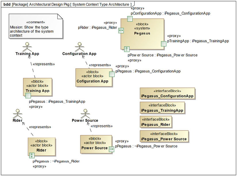
Figure 3.11: System type context as a block definition diagram

I created the stereotype «actor block» for blocks specifically representing actors because in Cameo, actors cannot have ports. The «represents» stereotype of dependency is used to explicitly relate the actor blocks and the actors. The «system» stereotype is from Cameo’s SysML profile in SysML::Non-Normative Extensions::Blocks package.

And – as I plan to use ports for actual connections – it can also be shown in an IBD, as in Figure 3.12.

This shows the system connected context and focuses on how the system and the actors connect to each other:

Figure 3.12: System connected context as internal block diagram

Copy system functions from use cases to systems block

To illustrate this, Figure 3.13 shows a block definition diagram with all the included use cases (as use case blocks) with their system functions and value properties and up-to-date Pegasus block:

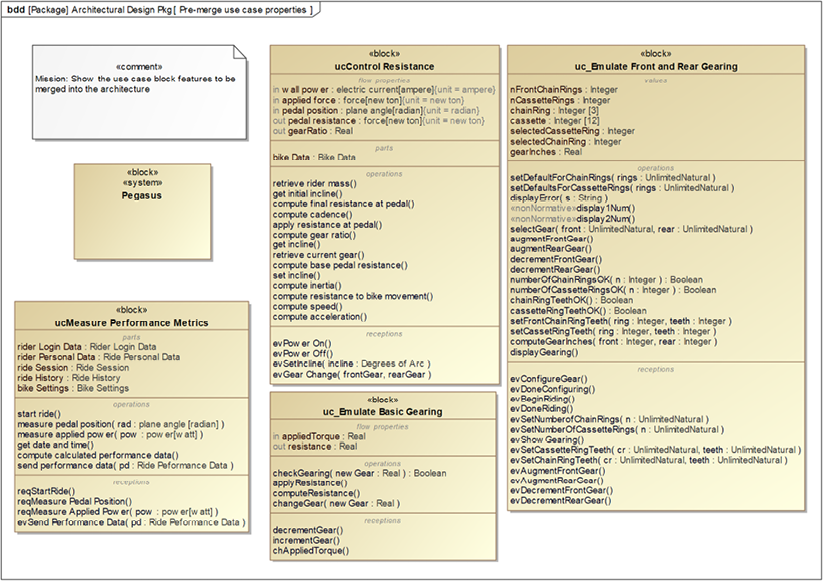
Figure 3.13: Use case block features to copy

It is important to perform a deep copy of the elements. Operations, signal receptions, flow, and value properties may reference types that are defined in the use case packages. This also includes reference and part properties owned by the copied elements. Simply copying the owning element doesn’t change that. We need to update the copy to point to the copied types as well.

Similarly, signal receptions will specify a signal that they receive, which is located in the use case packages. These signal receptions must be updated to reference the new copy of the signal in the architecture.

Figure 3.14 illustrates the problem:

Figure 3.14: The problem with copy

The signal reception evSendPerformanceData is copied from the ucMeasure Performance Metrics block to the Pegasus block. If we look at the specification of the signal reception, we see that it references the signal back in the use case package FunctionalAnalysisPkg::Measure Performance Metrics Pkg. Further, it carries a parameter, pd:Ride Performance Data, and that block defining the parameter is, once again, located back in the use case package. Since we are doing an architectural merge that includes both data and signals, these references must be updated to point to those elements in the architectural packages, as shown in Figure 3.15:

Figure 3.15: Updated copies to local referents

These copy updates aren’t difficult to do, although it can be a bit time-consuming.

Resolve system function conflicts

As you can see in Figure 3.13, the system block must merge a large number of functions. For the most part, there is no conflict; either the system functions are unique, such as Uc_MeasurePerformanceMetrics::send performance data() or they do the same thing in every usage. Nevertheless, a detailed inspection uncovers a few cases that must be considered.

For example, consider Uc_EmulateBasicGearing::changeGear(newGear: Real) and related functions like checkGearing(gear: Real) and the event ChangeGear(new gear: Real). These all have to do with the emulation of basic gearing. How do those functions relate to the specific front and rear gearing functions of the use case Emulate Front and Rear Gearing, such as selectGear(front: Unlimited Natural, rear: Unlimited Natural), augmentFrontGear(), augmentRearGear(), decrementFrontGear(), and decrementRearGear?

It could be that the changeGear function is called by the more specific functions that set the gearing for the front and rear chain rings, but does the training app need both the gearing (in gear-inches) and the currently selected front and rear? Gearing is a function of not only the gear ratio between the front and rear chain rings but also the wheel size, which the training app may not know. If the training app uses the current front and rear as a display option for the rider, does it still need the gearing value? Probably not, since the system itself calculates metrics such as power, speed, and incline, not the training app. In this case, it is enough to send the gearing event to the training app.

There is some subtlety in the various system functions and events. For example, the training app sends the event triggering the Uc_MeasurePerformanceMetrics::reqStartRide() event reception to indicate that it is ready to begin the ride and therefore ready to receive incoming data, while Uc_EmulateFrontandRearGearing::evBeginRiding() event reception is triggered by an event sent from the rider and not the training app. This points out just how important it is for every important system property to have a meaningful description! It would be very easy to get these events confused.

Copy system data from use cases to systems block

In addition to showing the system functions to copy, Figure 3.13 also shows the data, as value properties, to copy as well.

Resolve system data conflicts

Just as with the system functions, the data copies over without issue, but there are a few questions to resolve. Uc_EmulateFrontandRearGearing::gearInches: Real is the gearing ratio computed as a function of front and rear chain rings and wheel size. This is the same as Uc_ControlResistance::gearRatio: Real, so they can be merged into a single feature. We will use gearRatio: Real for the merged value property.

Copy interfaces from use cases to systems block

A number of interfaces were produced in the merged use case analyses. To start with, we will copy not only the interfaces themselves but also the events and any data types and schema passed as arguments for those events.

Figure 3.16 shows the copied interfaces in three different browsers, each showing different kinds of elements. The one on the left shows the interface blocks copied over and exposes their operations and flow properties. The middle browser shows (most of) the events copied over. The one on the right shows the copied data elements:

Figure 3.16: Interfaces copied to the architecture

Update interfaces to refer to copied system functions

The copied interfaces refer to events back in the originating use case analysis packages. In our use case analyses, we followed the convention that all services in these interfaces are modeled as event receptions, so we can limit our focus to ensure that the interface blocks refer to the event definitions in the architecture rather than to their definition in their original source, the use case analysis packages.

Update interfaces to refer to copied systems data

The system functions and event receptions of the Pegasus system block must all refer to the copied data types, not the original data types. This is also true for any flow properties in the interface blocks.

In this particular case, there is no use for user-defined types in the interfaces, so the data references are fine without changes.

Merge all interfaces for each actor

The last step in the recipe is to create the interfaces for the actors. In the previous chapter, we created interfaces not to the actors themselves during use case analysis but rather to blocks meant to serve as local stand-ins for those actors. The naming convention for the interfaces reflects that choice. For example, the interface block iUc_EmulateBasicGearing_aEBG_Rider is an interface between the use case EmulateBasicGearing and its local proxy for the Rider actor, aEBG_Rider. In this way, we can see which interfaces to merge together. All interfaces that contain a…Rider should be merged into an iPegasus_Rider interface. A similar process is followed for each of the other actors. This is because the system architecture must merge all the interfaces referring to the same actor. At the end, we’ll have an interface for each actor that specifies the interface between the system and the actor.

When it’s all said and done, Figure 3.17 shows the merged interfaces. Additional actors and interfaces may be uncovered as more use cases are elaborated, or they will be discovered as system design progresses:

Figure 3.17: Merged system interfaces

Pattern-driven architecture

Design patterns are “generalized solutions to commonly occurring problems,” (Design Patterns for Embedded Systems in C, by Bruce Douglass, Ph.D. 2011). Let’s break this down.

First, a design pattern captures a design solution in a general way. That is, the aspects of the design unique to the specific problem being solved are abstracted away, leaving the generally necessary structures, roles, and behaviors. The process of identifying the underlying conceptual solution is known as pattern mining. This discovered abstracted solution can now be reapplied in a different design context, a process known as pattern instantiation. Further, while each design context has unique aspects, design patterns are appropriate for problems or concerns that reappear in many systems designs.

To orient yourself to work with design patterns, you should keep in mind two fundamental truths:

• Design is all about the optimization of important properties at the expense of others (see the previous recipe about trade studies at the start of this chapter).
• There are almost always many different solutions to a given design problem.

With many design solutions (patterns) able to address a design concern, how is one to choose? Simple – the best pattern is the one that solves the design problem in an optimal way, where “optimal” means that it maximizes the desired outcomes and minimizes the undesired ones. Typically, this means that the important Qualities of Service (QoS) properties should be given a higher weight than those properties that are less important. A good solution, therefore, solves the problem by providing the desired benefits at a cost we are willing to pay. This is often determined via a trade study.

Dimensions of patterns

Patterns have four key aspects, or dimensions:

• Name: The name provides a way to reference the pattern independent of its application in any specific design.
• Purpose: The purpose of the pattern identifies the design problem the pattern addresses and the necessary design context preconditions necessary for its use.
• Solution: The solution details the structural elements, their collaboration roles, and their singular and collective behavior.
• Consequences: The pattern consequences highlight the benefits and costs from the use of the pattern, focusing on the design properties particularly optimized and deoptimized through its use. This is arguably the most important dimension because it is how we will decide which pattern to deploy from the set of relevant patterns.

Pattern roles

Structural roles are fulfilled by the structural elements (blocks) in systems engineering. A role can be defined as the use of an instance in a context. Design patterns have two broad categories of roles. The first is as glue. Roles of this type serve to facilitate and manage the execution of the collaboration of design elements of which the pattern is a part.

The second category is as a collaboration parameter. Design patterns can be described as parameterized collaborations. The parameterized roles are placeholders that will be replaced by specific elements from your design. That is, some design elements will be substituted for these roles during pattern instantiation; design elements substituting for pattern parameters are known as pattern arguments. Once the pattern is instantiated, the glue roles will interact with the pattern arguments to provide the optimized design solution.

Patterns in an architectural context

Architecture is design writ large. Architectural design choices affect most or all of the system and all more detailed design elements must live within the confines of the architectural decisions. As we said in the lead-in to this chapter, we are focused on six key views of architecture: subsystem and component view, concurrency and resource view, distribution view, data view, dependability view, and deployment view. Each of these views of architecture has its own rich source of design patterns. A system architecture is a set of architectural structures integrated with one or more patterns in each of these views.

This recipe will provide a workflow for the identification and integration of a design pattern in general; later recipes will use this pattern to address their more specific concerns.

Purpose

The purpose of design patterns is twofold. First, design patterns capture good design solutions so that they can be reused, providing an engineering history of good design solutions. Secondly, they provide a means by which designers can reuse existing design solutions that have proven useful.

Inputs and preconditions

The fundamental precondition for the use of design patterns is that there is a design problem to be solved, and some design elements have been identified.

Outputs and postconditions

The primary output of the application of design patterns is an optimized collaboration solving the design solution.

How to do it

The use of design patterns is conceptually simple, as can be seen in Figure 3.18. This simple flow somewhat belies the difficulty of good design because a good design generally has several interconnected patterns working together to optimize many aspects at once:

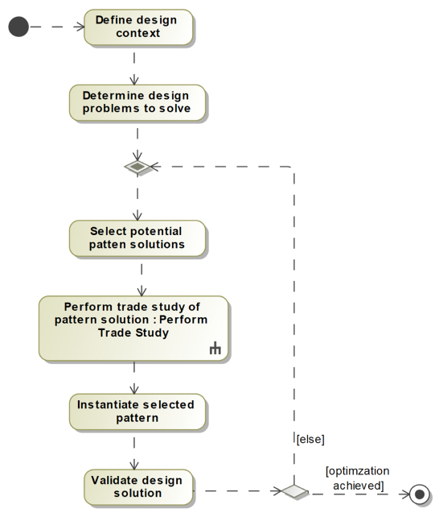
Figure 3.18: Apply design Patterns

Define design context

This step is generally a matter of defining essential elements of the design (sometimes known as the analysis model) without optimization. This includes the important properties including value properties, operations, state behavior, and relations. A general guideline I use is that this design context is demonstrably functionally correct, as demonstrated through execution and testing, before optimization is attempted. Optimizing too soon (i.e. before the design context is verified) generally leads to bad outcomes.

Determine design problem to solve

During the development of the design context, it is common to uncover a design issue which impacts the design qualities of services, such as performance, reusability, safety, or security. These design issues have often been solved before by other designers in many different ways.

Select potential pattern solutions

This step involves reviewing the pattern literature for solutions that other designs have found to be effective. A set of patterns is selected from the potential solution candidates based on their applicability to the design issue at hand, the similarity of purpose, and the aspects of the design that they optimize.

Perform trade study of pattern solution

Earlier in this chapter, we highlighted a recipe called Architectural Trade Studies. In some cases, a full-blown trade study may not be called for, but in general, this step of the recipe selects from a set of alternatives, which is what a trade study does. The observant reader will note that the icon used in Figure 3.18 for this step is a call behavior, which is a formal use of the earlier recipe.

Instantiate selected pattern

Once a pattern is selected, it must be instantiated. This is largely a matter of creating the structural and behavioral elements of the pattern and making small changes to some of the existing design elements to make them proper arguments for the design pattern parameters (aka refactoring).

Validate design solution

Once the pattern is instantiated, it must be examined for two things. First, before the pattern was instantiated, the design collaboration worked, albeit suboptimally (Step 1: Define design context). We want to verify that we didn’t break it so that it no longer works. Secondly, we applied the design pattern for a reason – we wanted to achieve some kind of optimization.

We must verify that we have achieved our optimization goals. If we have not, then a different pattern should be used instead or in addition to the current pattern. Patterns can be combined to provide cumulative effects in many cases.

Example

In this example, we will take a non-architectural design context. Later examples will apply the recipe to the Pegasus architecture for specific views of architecture.

Define design context

In this example, let’s consider a part of the internal design that acquires measured ride data from the power and pedal position sensors. See Figure 3.19:

Figure 3.19: Design collaboration (pre-pattern)

The design collaboration shows three device drivers: two for rider power (left and right sensors) and one for the pedal position for determining pedal cadence.

The Rider Power block gets the data from the two Power Sensor instances and aggregates it,

along with the current time into a Measured Power block that includes left and right power, the average of those two values, the time-averaged power, and a time stamp. The Rider Cadence block gets the pedal position and, using the real-time clock, can determine cadence. The Ride Data block then aggregates this data into an ordered collection Ride Datum constituting the information about the ride. The actual design incorporates much more computed data, such as computed speed and distance, but we’ll ignore that for now.

Determine design problem to solve

Some design optimization questions arise.

What’s the best way to get the data from the sensors in a timely way? It must be sampled fast enough so as not to miss peak power and cadence spikes (riders love that kind of data) and the data from the two different sources must be synchronized in terms of when they are measured. On the other hand, sampling at too high a rate requires more data storage and could limit the length of rides that can be recorded and stored.

Further, note the existence of multiple clients for the real-time clock. Is having all the clients request the current time the best approach?

Select potential pattern solutions

Let’s consider three design patterns that address the concern of getting data in a timely manner (from the author’s Design Patterns for Embedded Systems in C, 2011): the Interrupt Pattern, Opportunistic Polling Pattern, and Periodic Polling Pattern. The first creates an interrupt driver that notifies the clients when data becomes available. The second pattern requires the client to poll the data sources when it gets a chance. The last pattern is a modification of the second pattern in which the client is notified, via a timer interrupt, when it should go poll the data.

Figure 3.20 shows the Interrupt Polling Pattern. It is conceptually very simple: an interrupt handler installs a set of interrupt handler functions by first saving the old address in the interrupt vector table for the selected interrupt, and then it puts the address of the desired interrupt handler in its place. Later, when that interrupt occurs, the CPU invokes the selected interrupt handler function. There are some subtleties of writing interrupt handlers, but that’s the basic idea:

Figure 3.20: Interrupt pattern

Figure 3.21 shows the Opportunistic Polling Pattern. It works by having a Client, on whatever criteria it decides to use, invoke the OpportunisticPoller::poll() function.

The OpportunisticPoller then gets data from all the devices it polls (defined by NUM_POLL_DEVICES) and returns it to the Client. Easy peasy:

Figure 3.21: Opportunistic polling pattern

Figure 3.22 shows a specialized form of the previous pattern called the periodic polling pattern. In this pattern, the polling is driven by a timer; PeriodicPoller initializes and sets up the timer, which then invokes it with the specified period (ms are used here, but finer-grained polling can be supported with appropriate hardware resources):

Figure 3.22: Periodic polling pattern

The consequences of the patterns are summarized in Table 3.3:

Pattern	Pros (Benefits)	Cons (Costs)
Interrupt	Highly responsive to incoming data events	Can lead to data corruption unless interrupts are disabled during interrupt processing Can lead to data loss if the interrupt handler takes too long Can lead to processing starvation if data arrival is too frequent
Opportunistic Polling	Simple implementation Efficient use of processor resources since data is acquired when the processor is otherwise idle	No timeliness guarantee Slow polling can lead to data loss Less responsive to incoming data Data can be corrupted if interrupts are not disabled during polling
Periodic Polling	Relatively simple implementation Period is tunable for data arrival frequency	Data can be lost if the polling period is too long Processing starvation can occur if the frequency is too high Handling timer interrupt must be short or it can lead to data loss Data can be corrupted if interrupts are not disabled during polling

Table 3.3: Design patterns for timely data acquisition

Perform trade study of pattern solution

I won’t detail the process of conducting the trade study but instead provide a summary in Table 3.4. In this trade study, the Periodic Polling Pattern is selected:

Pattern	Criteria								Total Weighted Score
	Simplicity (W1 = 0.1)		Avoid Data Loss (W2 = 0.7)			Resource Efficiency (W3 = 0.2)
	MoE	Score		MoE	Score		MoE	Score
Interrupt	4	0.4		6	4.2		6	1.2		5.8
Opportunistic Polling	6	0.6		3	2.1		2	0.4		3.1
Periodic Polling	2	0.2		6	4..2		8	1.6		6

Table 3.4: Results of the trade study

The results in the table show that the Periodic Polling Pattern is selected as the best fit for our design.

Instantiate selected pattern

The next step is to instantiate the pattern. Conceptually, this is a matter of replacing the parameters of the pattern with design elements. In practice, this is often done via specialization of the parameters, so the design classes now inherit the structure and behavior required to integrate into the pattern. Additionally, there may be some small amount of reorganization (known as refactoring) such as the removal or modification of relations in the pre-pattern collaboration.

Figure 3.23 shows the instantiated design pattern. I’ve added colored shading to the pattern elements to highlight their use. The RiderData block subclasses the PeriodicPoller block; the RiderCadence and RiderPower both subclass the Device block. I’ve also elected to show the inherited features in the updated design blocks (indicated with a caret, ^). Those inherited operations will be implemented in terms of the existing functions within those specialized blocks. Further, the inherited data elements will not be used; the original data elements from the design elements will be used in their stead.

Note also that the original relations between RideData and RiderCadence and RideData and RiderPower have been deleted and subsumed by the single relation from RideData to Device; this relation applies to both RiderCadence and RiderPower since the latter two blocks are subtypes of Device.

In this case, NUM_POLL_DEVICES is 2. As mentioned previously, this change falls under the heading of refactoring:

Figure 3.23: Instantiated design pattern

Validate design solution

At this point, we reapply the test cases used to verify the collaboration previously and additionally look to ensure our objectives (as stated by the trade study criteria) have been addressed.

Subsystem and component architecture

The Subsystem and Component Architecture view focuses on the identification and organization of system features into the largest-scale system elements – subsystems – their responsibilities, and their interfaces. In the Architectural merge recipe, we learned how the system features may be aggregated into a singular system block and to create merged interfaces and associated logical data schema. In this recipe, we’ll look at how to identify subsystems, allocate functionality to those subsystems, and create subsystem-level interfaces.

So, what’s a subsystem?

We’ll use the definition from Agile Systems Engineering (see Agile Systems Engineering by Bruce Douglass, Ph.D., Morgan Kaufman Press, 2016):

Subsystem: An integrated interdisciplinary collection of system components that together form the largest-scale pieces of a system. It is a key element in the Subsystem and Component Architecture of the system.

Note that the definition includes the notion of a subsystem being interdisciplinary. This means that you will not define a “software subsystem,” an “electronics subsystem,” and a “mechanical subsystem,” although in a particular subsystem, one engineering discipline may dominate the design. Rather, subsystems are focused around tightly coupled requirements and coherent purpose and then implemented with some combination of engineering disciplines. The engineering contribution of an engineering discipline to a subsystem is referred to as a facet to distinguish it from subsystems and components. Discipline-specific facets are discussed in Chapter 4, Handoff to Downstream Engineering.

Modeling a subsystem in SysML

In SysML, a subsystem is just a block, although it is common to add a «Subsystem» stereotype. This can be found in the Cameo SysML library in the SysML::Non-Normative Extensions::Blocks package. It is common – although by no means required – to connect subsystems together by adding connectors between ports on the subsystems. In this book, we will use SysML proxy ports for that purpose.

More specifically, we will use proxy ports for dynamic connections, that is, connections that require the exchange of flows, such as control, energy, fluid, or data, whether discrete or continuous. For static connections, such as when mechanical pieces are bolted together, we will use associations between the blocks and direct connectors between the parts.

Block definition diagrams will be used to show the subsystem types and properties. This view is known as the system composition architecture. Internal Block Diagrams will show how the usages of the blocks are connected together to create an operational, running system. This latter view is sometimes known as the system connected architecture.

Choosing a subsystem architecture

It is important to remember that many subsystem architectures can achieve the same system-level functionality. The selection of a specific subsystem architecture is always an optimization decision.

Some of these optimization criteria are typically stated as “guidance” or “rules of thumb,” but they are really stating properties you’d like a good subsystem architecture to enhance. Some goals and principles for the creation of good subsystems are:

• Goals of subsystem and component architecture:
  • Reuse proven subsystem architectural approaches (patterns)
  • Support end-to-end performance needs easily
  • Minimize system recurring cost (cost per shipped system)
  • Maximize ease of maintenance
  • Minimize the cost of repair
  • Leverage team skills
  • Leverage existing technology and intellectual property (IP)
• Principles of subsystem and component architecture selection:
  • Coherence: Subsystems should have coherent intent and content
  • Contractual interaction: Subsystems should provide a small number of well-defined interfaces and services
  • Encapsulation: Tightly-coupled requirements and features should be in the same subsystem
  • Collaboration: Loosely-coupled requirements and features should be in different subsystems
  • Integrated teams: A subsystem is typically developed by a well-integrated interdisciplinary team
  • Reusability: Good subsystems can be reused in other, similar systems without requiring other contextual elements

Purpose

The purpose of creating this architectural view is to identify the subsystems and their responsibilities, features, connections, and interfaces. This provides a large-scale view of the largest-scale pieces of the system into which more detailed design work will fit.

Inputs and preconditions

The inputs include a set of requirements defining the overall system functionality. It is recommended that these requirements are organized into use cases, but other organizations are possible.

This input is a natural consequence of the recipes of Chapter 2, System Specification.

Additionally, the set of external actors – elements outside the system with which the system must interact – have been defined. This input is a natural consequence of the recipes of Chapter 2, System Specification.

Finally, an initial set of system functions, flows, and information has been identified through requirements or use case analysis and merged into a system block via the Architectural merge recipe or its equivalent.

Outputs and postconditions

At the end of this recipe, a set of subsystems have been identified, including their key system functions, data, and interfaces.

How to do it

The recipe workflow is shown in Figure 3.24:

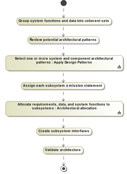
Figure 3.24: Create subsystem and component architecture

Groups systems functions and data into coherent sets

This task groups system features together by commonality. That commonality can be along different dimensions, such as a common flow source (sensors or system inputs), similar processing/transformation, similar use, reuse coherence (things that tend to be reused together), and dependability level (high-security or high-safety features tend to be grouped together).

These sets form the basis on which subsystems can be identified.

Review potential architectural patterns

As mentioned, there are many ways of organizing subsystems. The book, Real-Time Design Patterns by Bruce Douglass, Ph.D., Addison-Wesley Press (2003) identifies a number of popular subsystem patterns, such as the Microkernel, Layered, and Hierarchical Control patterns. Select one or more patterns that have the desired system properties.

Select a subsystem and component architectural pattern

This step is actually a reference to the Pattern-driven architecture recipe. This recipe details how to quantitatively select from a set of alternative technical approaches.

Assign each subsystem a mission statement

Once a set of subsystems is identified, each should be given a description that identifies the criteria for deciding whether or not it should host or contribute to a system capability.

Allocate requirements, data, and system features to subsystems

This step allocates system functionality, flows, and data to the subsystems. This is sometimes a little tricky and so is implemented by the next recipe in the book, Architectural allocation.

Create subsystem interfaces

System functionality will be provided by a collaboration of subsystems, and this requires those subsystems to communicate and coordinate. The subsystem interfaces specify the services and flows that will be used to accomplish this. They often tie in with the system-actor interfaces at one end or the other, but not necessarily. The system interfaces are created by the recipe Specifying logical system iInterfaces in the previous chapter.

Validate architecture

This step examines the resulting subsystem architecture to ensure that it can deliver the necessary system functionality and also that it achieves the optimization goals used to select the subsystem pattern.

Example

In this example, we’ll create an architecture for the Pegasus system based on some of the use cases considered in previous recipes, such as Emulate Front and Rear Gearing, Control Resistance, Measure Performance Metrics, and Manually Adjust Bike Fit.

Groups systems functions and data into coherent sets

The functionality of the system can be grouped by common purpose and capability. A good way to do this is by looking at the system use cases, as we did in Chapter 2, System Specification. Similar to how we treat requirements and system functions, either a use case can be directly allocated to a single subsystem or it must be decomposed into subsystem-level use cases that can be so allocated. This decomposition is best represented with the «include» relation. Any subsystem-level use cases created in this way will be tagged with the «Subsystem» stereotype.

For the most part, elements added to the system block during the Use case merge recipe can just be moved to the appropriate subsystems. If you want to capture your reasons for the allocation, SysML provides a special kind of comment, «rationale», which you can anchor to the elements. You can even create element groups (in the right-click menu in Cameo for model elements). Element groups anchor elements and have a criterion property where you can add the rationale for the grouping.

To begin with, let’s consider a set of use cases (Figure 3.25). Note that while this set encompasses a wide range of system capabilities, it doesn’t include all capabilities. We recommend this work is done incrementally, and additional use cases – and even subsystems – can be added later as the need for them is identified:

Figure 3.25: Set of use cases for subsystem allocation

Some of these use cases are likely to be allocated to a single subsystem. For example, the Manually Adjust Bike Fit use case might be allocated to a single Mechanical Frame. Others are likely to use multiple subsystems. For example, the Control Incline use case might be decomposed into subsystem-level use cases that map functionality to the User Input and Mechanical Frame subsystems. The exact decomposition will, of course, depend highly on the set of subsystems upon which we decide.

Review potential architectural patterns

There are many potential subsystem patterns from which to choose. From Buschmann et al., the Model-View-Controller and Microkernel architecture patterns seem potentially viable, although the former is more of a design collaboration-level pattern than an architectural design pattern. From the previously mentioned Real-Time Design Patterns book, the Layered, Channel, and Hierarchical Control patterns are possibilities.

Select a subsystem and component architectural pattern

Using the workflow from the previously presented Pattern-driven architecture recipe, we select the Five-Layer Architecture Pattern from the Real-Time Design Patterns book as our base pattern. We will modify it to use subsystems rather than packages, as in the original, and to replace Abstract OS Layer with Abstract Common Services Layer, as it seems more relevant to our design. See Figure 3.26:

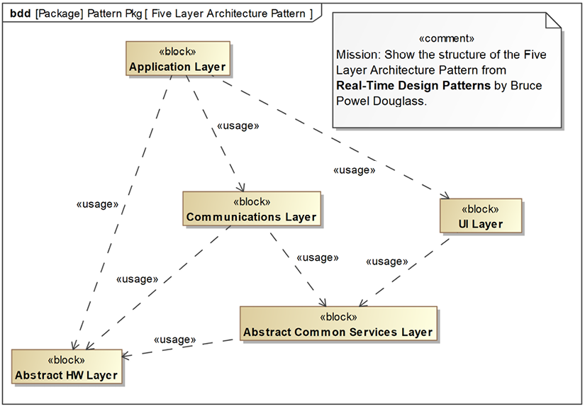
Figure 3.26: Modified Five-Layer Architecture Pattern

Each of the blocks in the pattern may have multiple instantiations for peers (such as multiple Application Layer elements) or may have an internal sub-subsystem structure (which we will refer to as simply “subsystems”).

Each of these blocks in the pattern has its own purpose and scope.

Application layer

This layer contains features at the application level, so system features (data and services) such as Ride and Rider metrics and properties would reside in this layer.

UI layer

This layer contains elements for the system user input. This includes the selection and display of current gearing, for example. Most display features actually reside on the third-party training apps, so the system itself has a limited UI.

Communications layer

The system requires Bluetooth and ANT+ communications protocols, setting up sessions, and so on. All those features reside largely in this layer.

Abstract common services layer

This layer contains common services such as data storage and data management and also electric power delivery.

Abstract HW layer

This layer focuses on electronic and mechanical aspects; frame adjustment, drive train, various sensors, and so on all reside here. This is likely to have peer instantiations and substructure.

The above discussion explains the pattern per se. Now, let’s look at the pattern instantiation.

The set of six proposed primary subsystems is shown in Figure 3.27 along with their high-level parts (also identified as subsystems).

Figure 3.27: Pegasus proposed subsystems

We can create a “connected architecture” view showing how we expect the subsystems to connect. This will evolve as we elaborate the architecture and allocate functionality. Figure 3.28 shows the connected architecture showing only the high-level subsystems. Figure 3.29 shows the same view but with the internal structure we’ve identified so far. In both cases, I used Cameo’s Symbol Properties feature to change the line color and width for the electrical power connections to differentiate them. The connections are notional at this point and may change as we dive into the details of the architecture:

Figure 3.28: Pegasus high-level connected architecture

Figure 3.29: Pegasus detailed connected architecture

Assign each subsystem a mission statement

The mission statement for each subsystem is added to the Description field of the subsystem block. The mission statements for the high-level subsystems are provided in Table 3.5:

Subsystem	Mission Statement
Mechanical Frame	This subsystem provides the physical system structure and rider adjustment features – all of which are assumed to be strictly mechanical in nature – and also the inclination delivery/monitoring capability, which is planned to be motorized. This subsystem is envisioned to primarily consist of mechanical and electronic aspects.
Electric Power Delivery	This subsystem is responsible for receiving wall power and distributing managed electrical power to the other subsystems. This includes low amperage power for digital electronics, moderate amperage power for the motorized inclination capability, and high amperage power for the rider power and resistance. This subsystem design is envisioned to be dominated by electronic aspects.
Comms	This subsystem is responsible for all communications with external devices. At this time, this includes low-power Bluetooth and ANT+ communications protocols. This includes the physical layer through the network layer of the OSI protocol stack. The initial concept for this subsystem includes one or more smart communications processors to manage the communications activity. This subsystem is envisioned to consist primarily of digital electronics and software.
Main Computing Platform	The main computing platform contains the primary computing electronics and software for the system. It manages rider-level applications such as controlling and monitoring rides and sensor data, system configuration (including motor transfer function tuning and rider settings), and data management. This subsystem is envisioned to be primarily software and digital electronics hardware.
Rider Interaction	This subsystem provides the primary user interface (except for pedals) for the system, including shift and brake levers, and a display of the currently selected gearing. This system is envisioned to include mechanical, electronic, and software aspects.
Power Train	This subsystem manages the pedal assembly, the monitoring of rider power and pedal cadence input, and the creation of resistance to pedaling, under the direction of the Main Computing Platform subsystem. This system is envisioned to include mechanical, electronic, and software aspects.

Table 3.5: Subsystem missions

Allocate requirements and system features to subsystems

This task is complex enough to have its own recipe, Architectural allocation, later in this chapter. The example is elaborated on in that section.

Create subsystem interfaces

This task is complex enough to have its own recipe, Creating subsystem interfaces from use case scenarios, later in this chapter. The example is elaborated on in that section.

Architectural allocation

The recipes for functional analysis of use cases have multiple outcomes. The primary outcome is a set of high-quality requirements. The second is the identification of important system features – system functions, data, and flows. The third outcome is the identification of interfaces necessary to support the behavior outlined in the use case. This recipe focuses on allocating the first two of these to the subsystem architecture.

Purpose

The purpose is to detail the specification of the subsystems to get ready to hand off those specifications to the interdisciplinary subsystem teams for detailed design and development.

Inputs and preconditions

A set of requirements and system features have been identified, and a subsystem architecture has been created such that each subsystem has a defined mission (scope and content).

Outputs and postconditions

The primary outcome of this recipe is a specification for each subsystem that includes:

• System requirements allocated directly to the subsystem
• Subsystem requirements derived from system requirements, which are then allocated to the subsystem
• System features allocated directly to the subsystem
• Subsystem features derived from system features, which are then allocated to the subsystem

How to do it

This recipe is deceptively simple. The tasks are straightforward, although difficult to completely automate. This task can take a while to perform because there are often many requirements and features to allocate. The basic idea is that given the selected subsystem structure, either allocate a feature directly, or decompose that feature into subparts that can be so allocated. The workflow is shown in Figure 3.30:

Figure 3.30: Architectural allocation

Decompose non-allocable requirements

Requirements can sometimes be directly allocated to a specific subsystem. In other cases, it is necessary to create derived requirements that take into account the original system requirements and the specifics of the selected subsystem architecture. In this case, create derived requirements that can be directly allocated to subsystems. Be sure to add «deriveReqt» relations from the derived requirements back to their source system requirements.

Allocate system requirements

Allocate system requirements to the subsystems. In general, each requirement is allocated to a single subsystem, so in the end, the requirements allocated to each subsystem are clear. The set of allocated system requirements after this step is normally known as subsystem requirements.

Decompose non-allocable system functions and data

Some system features – which refer to operations, event receptions, flows, and data – can be directly allocated to a single subsystem. In practice, many cannot. When this is the case, the feature must be decomposed into subsystem-level features that trace back to their system-level source feature but can be directly allocated to a single subsystem.

Allocate system functions and data

Allocate system features to subsystems. That is, each system function now becomes a subsystem function allocated to a single subsystem, or it is decomposed to a set of subsystem functions, each of which is allocated. Similarly, system event receptions must be allocated to some subsystem and, often, this results in new subsystem event receptions being added elsewhere in the architecture to support the subsystem collaboration required to fulfill the system functionality needs. System flows and data must also be allocated to subsystems.

Example

In real system development, this recipe can take a substantial amount of time, not due to the complexity of the task but because of the large number of system requirements and features requiring allocation.

To keep the example manageable for the book format, we will focus on a subset of the requirements and system features identified in the use cases under consideration for this book:

Figure 3.31: Requirements selected for allocation

Figure 3.31 shows the set of requirements for a single use case, Compute Resistance. In the interests of brevity, we will decompose and allocate a subset of these requirements.

Decompose non-allocable requirements

As mentioned, some requirements must be decomposed into derived requirements before allocation. This is because these requirements are partially met by different subsystems. In this case, a set of derived requirements must be created that are collectively equivalent to the original requirement but are of appropriately narrow focus so that they can be directly allocated. This is modeled with the «deriveReqt» relation, going from the derived requirement to the originating requirement:

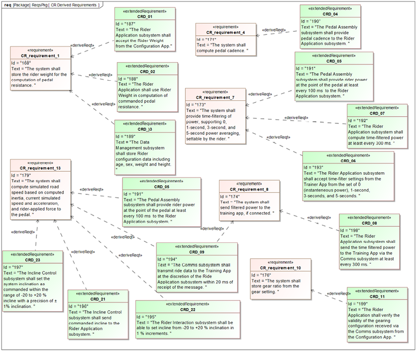
Figure 3.32: Some derived requirements

Figure 3.32 shows some of the requirements created during the derivation process. I color-coded the original system requirements and the derived requirements as a visual aid. Again, note the directions of the relations.

The figure shows a number of the system requirements decomposed into subsystem requirements. For example, CR_requirement_7 states “The system shall provide time-filtering of power, supporting 0, 1-second, 3-second, and 5-second power averaging, settable by the rider.” This results in three derived requirements:

• CRD_05: The Pedal Assembly subsystem shall provide rider power at the point of the pedal at least every 100 ms to the Rider Application Subsystem.
• CRD_06: The Rider Application subsystem shall accept time-filter settings from the Trainer App from the set of 0 (instantaneous power), 1-second, 3-second, and 5-second).
• CRD_07: The Rider Application shall compute time-filtered power at least every 300 ms.

It can be cumbersome to show derived requirements diagrammatically for large numbers of derived requirements. An alternative is to construct a matrix showing originating and derived requirements. Such a matrix is shown in Figure 3.33:

Figure 3.33: Derived requirements matrix

As we create new subsystem requirements, we need a place to put them. In this example, we’ll create SubsystemRequirementsPkg under RequirementsAnalysisPkg::RequirementsPkg for this purpose. We may later decide to create a package per subsystem within SubsystemRequirementsPkg if the number of derived requirements grows large enough to justify it.

Allocate system requirements

Allocation means “assignment” in the sense that a subsystem is expected to implement its allocated requirements. This can be done diagrammatically, but in this case, we’ll do this using an allocation matrix, as shown in Figure 3.34. In this matrix, the allocation relation goes from the subsystem to the requirement. The matrix itself is located in DesignSynthesisPkg::ArchitecturalDesignPkg in the model, but other locations are possible. The matrix layout used Block as the from element type, Requirement as the to element type, and Allocation as the cell element type.

The actual allocation is performed by walking through the requirements and creating an allocation relation from the subsystem to the requirement. Figure 3.34 shows the system and derived requirements and their allocation for this subset:

Figure 3.34: Subsystem requirements allocation matrix (subset)

Note that the matrix uses the convention that system requirements requiring decomposition are shown as allocated to the Pegasus block in Figure 3.34, while system requirements that are directly allocable are allocated directly to the subsystem. The requirements derived from the decomposed requirements are allocated to individual subsystems. In the figure, system requirements are all named CR_requirement_<#> (the CR indicating the Control Resistance use case), while the derived requirements are named CRD_<#>.

Also note that, for the most part, the high-level subsystems – that is, those that contain subsystems themselves – don’t have allocated requirements, although their internal parts do. This is not uncommon. Thus, the Main Computing Platform, Power Train, and Rider Interaction subsystems don’t have requirements directly allocated to them, but each contains nested subsystems that do.

Finally, note that the matrix is sparsely populated. This is because it only shows requirements from a single use case. As use cases are added, this matrix will become much more densely populated.

The matrix is shown with the subsystems as the rows because it fits better into the book format. Normally, the systems would be the columns because I prefer to have matrices with more rows than columns for readability within the modeling tool.

Allocate system functions and data

For the system features, we’ll use the features we allocated to the system object during the Architectural merge recipe earlier in this chapter. The set of system features is shown in Figure 3.35. Note the Pegasus block is shown three times with different features shown for readability reasons.

The view on the left shows flow and value properties, while the views on the right show operations and event receptions:

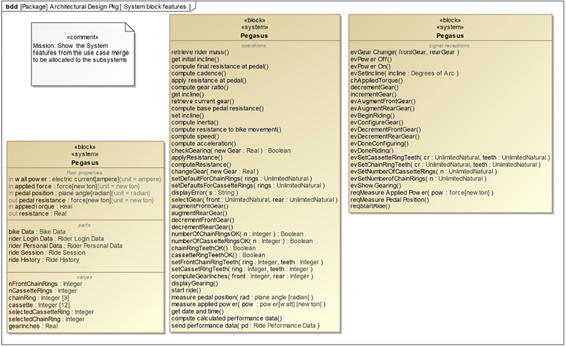
Figure 3.35: System features for allocation

The standard way of performing the allocation following the architectural merge is to move (in Cameo, drag and drop) the system feature to the appropriate subsystem. Any system features that remain after that initial pass are then decomposed and allocated (the last step in the recipe).

It may happen that a system feature cannot be allocated, not because it must be decomposed but because there is no appropriate subsystem. In this case, the missing subsystem must be added. It can also happen that at the end of the entire recipe, there are subsystems to which no requirements or features have been allocated. This simply means that subsystem isn’t being used in the current iteration but might be in future iterations. Generally speaking, at the end of the recipe, all subsystems should have features allocated to them or serve another purpose (such as organizing and containing smaller subsystems).

Figure 3.36 shows the result of this step. Several of the subsystems have value properties, event receptions, and operations allocated to them:

Figure 3.36: Initial allocation of system features

Decompose non-allocable system functions and data

In this example, the only system feature not directly allocated is the operation Send_Performance_Data. We have decomposed this service into:

• Gather_Performance_Data (allocate to the Rider Application subsystem)
• Construct_Performance_Data_Msg (allocate to the Rider Application subsystem)
• Send_Msg (allocate to the Comms subsystem)

While we’re doing that, we note that we also need Receive_Msg and Dispatch_Msg system functions for the Comms subsystem.

To then allocate these created system features, leave the decomposed system feature in the system block and directly add the created features to the appropriate subsystem. Then add relations from the original feature to the derived features. In this case, we’ll use the «derive» relation (as opposed to «deriveReqt» since these are system properties, not requirements). This is shown graphically in Figure 3.37. If you look closely, you can see the relations not between the blocks themselves, but the operations shown:

Figure 3.37: Some derived system features

An easier way to visualize these relations is with a dependency matrix, as shown in Figure 3.38:

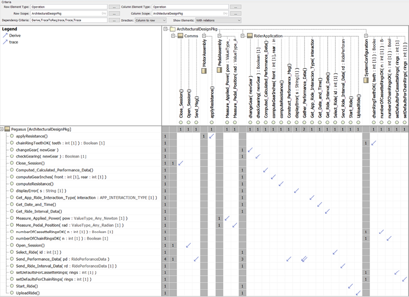
Figure 3.38: Dependency matrix showing derived relations between operations

Creating subsystem interfaces from use case scenarios

There are many methods by which subsystem interfaces can be created. For example, a common approach is to refine the black box activity diagrams from the use case analyses into so-called white box activity diagrams with activity partitions representing the subsystems. When control flows cross into other swim lanes, the flow or service invocation is added to the relevant subsystem interface. Another common approach is to do the same thing but use the use case sequence diagrams rather than the activity diagrams. The advantage of these approaches is that they tie back into the use case analysis. It is also possible to create the interfaces de novo from the allocation of system features to the subsystems.

This recipe focuses on using sequence diagrams in the creation of the system interfaces. One advantage of this approach is that this approach can leverage sequence diagrams created from the execution of the use case models that may not appear on the activity diagram. Further, many engineers use the activity diagrams as the starting point but the state machines become the normative specification of the use case; that is, the activity diagrams are not fully fleshed out but the state machines are. In such cases, this approach is superior to basing the interface definitions on the incomplete activity diagrams.

Purpose

The purpose of this recipe is to develop the interfaces between the subsystem so that the subsystem teams can design with an understanding of the flows and services they must provide to and require from other subsystems. These interfaces are still logical and reference essential aspects and are largely technology independent. These interfaces will be refined into physical interfaces that explicitly expose technical details in recipes discussed in the next chapter.

Inputs and preconditions

The inputs include the identified set of subsystems to which system features have been allocated. In addition, each referenced use case has a set of black box sequence diagrams showing the interaction of the use cases and the actors.

Outputs and postconditions

The primary outcome of the recipe is the set of interfaces (as interface blocks) defining the logical flows and service invocations between the subsystems and between the system and the actors. A part of that definition will be the logical data schema for flows and service parameters.

How to do it

This recipe is straightforward, although it can be a little tedious to perform by hand in many scenarios. Figure 3.39 shows the workflow.

In any case, the outcome is a set of subsystem interfaces that support the necessary interactions for the architecture to realize the use case behaviors:

Figure 3.39: Creating subsystem interfaces from use case scenarios

Add owner to hold white box scenarios

In Cameo, the owner of a sequence diagram must be a classifier (unlike Rhapsody, which allows packages to directly own sequence diagrams).

In this case, the logical choice for the owner of the architectural white box scenarios is the architectural system context block that has the system and the architectural actor blocks as parts. This is the System Context block shown in Figure 1.29 in the Architecture 0 recipe.

Create scenario

Either copy an existing interaction in the browser or create an entirely new sequence diagram for the owner. If you create a new sequence diagram for the context block, Cameo will pop up a dialog asking you to select which parts you’d like to include. This will be done for each scenario in every included use case. I like to ensure the same ordering of all the lifelines for all the scenarios, so I generally prefer to copy the interaction and its own sequence diagram to retain the same ordering. This makes it easier to compare sequence diagrams later.

As a part of this step, you can add a «refine» relation from the new architectural scenario (interaction) back to the original use case scenario (interaction) it is elaborating. In Cameo, it is a simple task to create a matrix showing which architectural interactions elaborate which functional analysis interactions based on this relation.

I find it useful to add _WB (for “white box”) to the name of the new sequence diagram to ensure that it isn’t confused with its source.

Replicate the source scenario but with the real actors and subsystems

In this step, we will recreate the messages from the actor block to the use case and from the use case to the actor block in the new scenario. What will be different is that the architectural actor block will be used, and the message termination inside the system will be some specific subsystem rather than the use case or use case block.

Add necessary subsystem interaction messages

This is a “magic step” in the recipe and requires the engineer to decide how the subsystem interaction should occur to realize the use case messages at the black-box level. The engineer must consider the requirements, data, and services allocated to the subsystems and create messages to support an interaction that will use them to achieve the system-level objective.

Create subsystem ports if missing

If there is at least one message between a subsystem and another, or between a subsystem and an actor, then the subsystem must have a port to support that message exchange. If the message is between a subsystem and an actor, then it will require a port on the system block. In this case, the subsystem’s port will connect to the system’s port, and then in turn, the system’s port will connect to the actor’s port. It is a good idea to set each block’s isEncapsulated property to true, as this enforces the rule that a block’s parts may only be accessed through the composite block’s properties. This is especially true for the system block. Unfortunately, it doesn’t appear to be possible to set this as a project option, so it must be done separately for each block. Once set, the Cameo rules validator will detect and report any such violations (see the Analyze > Validation > Validate menu).

Create subsystem interfaces if missing

Once the white box sequence diagram is updated, interfaces can be created wherever two subsystems exchange messages. This means that in the architecture, they will relate via a connector. I recommend this connection is done via ports typed by interfaces that support those messages. These interfaces will include any operations, event receptions, and flow properties that cross the system boundary.

Update interfaces with messages

In the previous step, we added interfaces whenever there was at least one message exchanged between a pair of subsystems or a subsystem and an actor. In this step, we will add the messages as signal receptions. We will stereotype them as «directedFeatures» in the interface blocks if we’re using proxy ports.

This cycle is repeated for all functional analysis scenarios included in the architectural design.

Example

For this example, we will focus on the scenarios from two use cases: Measure Performance Metrics and Control Resistance. These scenarios show the interactions between actor blocks (acting as proxies for the actual actors) and the selected use case.

Add owner to hold white box scenarios

If the model doesn’t already have a System Context block that has composition relations to the Pegasus and the architectural actor blocks, we will do it now. This block will own the white box interactions, which will in turn own the sequence diagrams.

Create scenario

The first scenario is Measure Performance Metrics Black Box View 1, which was derived from the use case activity diagram. The original sequence diagram is shown in Figure 3.40. We show it here as reference; we won’t modify it, but we will replicate it in the upcoming steps:

Figure 3.40: Original use case scenario

In the containment tree, also open the newly created sequence diagram showing all the subsystems as lifelines. In Cameo, you can right-click a diagram tab and select New Vertical Group to show diagram windows side by side.

Replicate the original scenario but with system actor blocks and subsystems

The easiest way to work is to open the new and original sequence diagrams side by side (Figure 3.41):

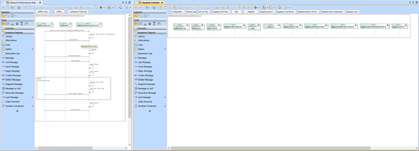
Figure 3.41: Ready to replicate messages

This step is easy; using the original scenario as guidance, add the same messages to the new scenario. The slightly tricky part is deciding which subsystem should be the sender or receiver lifeline. For this scenario, the lifeline receiving and sending the events to and from the Training App lifeline will be the Comms subsystem. Deciding where the “messages to self” go is only a little harder. If the services have to do with communications per se, then they will be put on the Comm subsystem lifeline. In this case, all the other messages to self will be put on the Main Computing Platform lifeline.

The sequence diagram now looks like this (Figure 3.42):

Figure 3.42: Scenario replicated

You will note that a miracle occurs between the Comm subsystem receiving a message and the Main Computing Platform doing something. That is because we are missing the messages between those subsystems; their identification and elaboration are outcomes of this recipe.

Add necessary subsystem interaction messages

As we go down the sequence, we need to add messages between the subsystems so that we can coordinate their actions and collectively perform the overall system interaction with the actors. It also happens that we may discover discrepancies in the original interaction, such as missing messages to or from an actor or data that must be passed with an existing message. Since we are defining the actual logical messages within the architecture, we will address those defects here.

The result of this step is a white box sequence diagram that shows the interaction of the subsystems with other subsystems and the actors. Some of these messages will be realized by the operations allocated to the subsystem during the Architectural allocation recipe earlier in this chapter. Others will be new.

Figure 3.43 shows the previous sequence diagram elaborated with the messages between the subsystems to complete the architectural flow. If we then repeat this for all the scenarios under consideration, we can use that to form the basis of the architectural interfaces:

Figure 3.43: White-box scenario measure performance metrics

Repeating that elaboration process for the other three scenarios – Control Resistance, Process Pedal Inputs, and Execute Physical Model – results in Figure 3.44, Figure 3.45, and Figure 3.47:

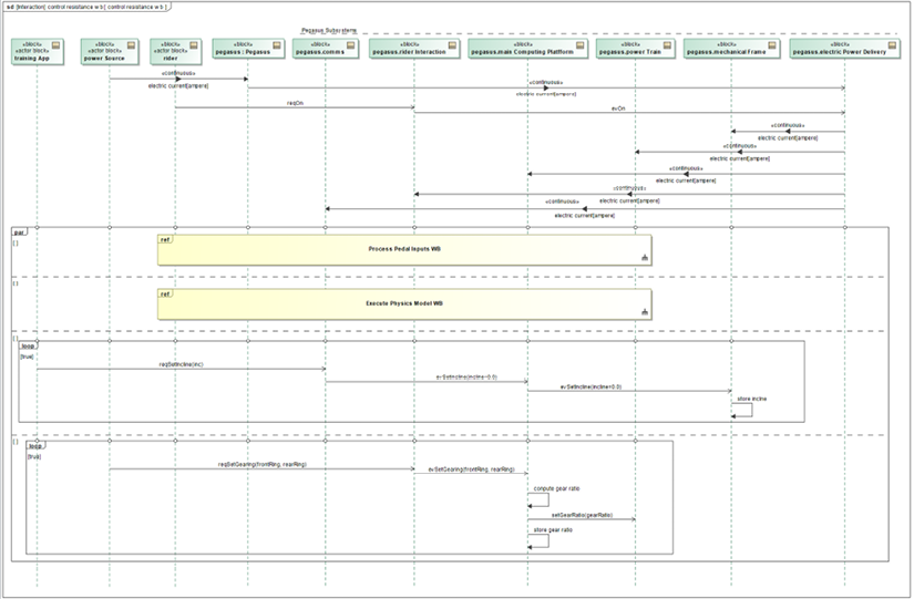
Figure 3.44: White-box scenario control resistance

Figure 3.45: White-box scenario process pedal inputs

Note the item flows on a few of the messages in Figure 3.45. This is done in Cameo by selecting the message and clicking on the item flow manager icon in the popup quick toolbar. However, in Cameo, this can only be added when the flow item is already defined in the model as occurring between the elements represented by the lifelines. One natural place to do that is in the internal block diagram, as shown in Figure 3.46:

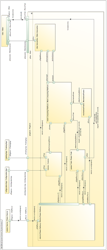
Figure 3.46: IBD with flow items

Figure 3.47: White-box scenario execute physics model

Create subsystem ports if missing

Wherever at least one message exists between elements in the white box scenarios, there must be a port pair supporting that message exchange. The ports necessary to support the white box scenarios are shown in Figure 3.46.

Ports are named with a p followed by the name of the target element to which they will connect. The Comms port that will connect to the Main Computing Platform subsystem is thus named Comms.pMainComputingPlatform. The ports for delivery of power from the Electric Power Delivery subsystems are flow ports because they each only deliver a singular flow without the invocation of services.

Create subsystem interfaces if missing

In the elaboration of the white box scenarios in the example, we have identified interactions between a number of subsystems and added port pairs to support the messaging.

Interface blocks are named with an i followed by the name of the unconjugated user of the interface block, an underscore, and the name of the conjugated side of the connection. Consider the interface block is named iMainComputingPlatform_Comms; its naming indicates that the MainComputingPlatform.pComms port uses the interface block in its normal form but the Comms.pMainComputingPlatform port uses the interface block in conjugated form.

Update interfaces with messages

This step adds the messages sent across the ports to the interface blocks. These messages are the messages on the white box sequence diagrams. Note that, by convention, we are using asynchronous messages between the subsystems and between the system and the actors to define these logical interfaces. Since these are proxy ports, SysML requires us to stereotype these messages in the interface blocks as «directedFeatures». Once this stereotype is applied, the feature direction property appears and the message direction can be specified as provide, required, or providedrequired.

In this example, Figure 3.48 shows interface blocks and their services identified from the scenarios examined in this example:

Figure 3.48: Derived subsystem interface blocks

Specializing a reference architecture

In this recipe, we will discuss the first of two approaches for using a reference architecture.

What is a reference architecture?

In Chapter 1, Basics of Agile Systems Modeling, we defined architecture as “the set of strategic design optimization decisions for the system.” The use of the word strategic here is important; these are design decisions that affect most or all subsystems and impact the overall performance and structure of the system. In the previous discussions, we went on to identify the six key views of architecture: the subsystem and component view, the concurrency and resource view, the distribution view, the data view, the dependability view, and the deployment view.

In the Pattern-driven architecture recipe in this chapter, we talked about how an architecture is an instantiation of patterns. In fact, a systems architecture is an integration of one or more patterns in each of the architectural viewpoints.

A reference architecture is an extension of this concept. A reference architecture is a pattern writ large; it is a combination of a set of patterns to define a master pattern for the architecture of a type of system, such as perhaps an aircraft, satellite, or medical ventilator. That means that a reference architecture generally cannot be used as-is. It must be instantiated for use to create specific system designs. In this recipe, I will call that process specializing the reference architecture.

Why would I use a reference architecture?

There are six main reasons for using a reference architecture.

Frame of reference

A reference architecture provides a frame of reference to get an overview of a system’s structure, organization, functionality, and behavior. Because the principles of the system’s architecture are defined by the reference architecture to which it complies, it becomes easier to understand how a system is put together and how to effectively maintain, update, and enhance the system.

Interoperability

Systems are almost never standalone islands of capability. They fit into both an engineering and an operational context. In the engineering context, we have common development tools, plug-and-play components, and other common elements to assist in design and development. In the operational context, we have concerns about the use, maintenance, and sustainment of the system in operation – including the dev sec ops culture, automation, and integration of the system into enterprise architectures.

Interoperability is also important when you have a portfolio of related systems. You will gain economy-of-scale advantages with common usable elements and designs across a portfolio. Reference architectures are a way of specifying that commonality.

Reuse of effective architectures

The vast majority of systems are rehashing or slight improvements on the existing design. We have decades of experience developing avionics and medical systems, for example. As we gain industrial experience with such systems, we learn which architectures are effective in practice (and not just in theory) and which are not. Complying with a reference architecture enables gaining these benefits with relatively little effort.

Benchmarking

Comparing metrics and outcomes of different systems is made easier when they are specializations compliant with a common reference architecture.

Regulatory compliance

In regulated industries, such as aerospace, automotive, and medical, gaining regulatory approval is crucial to a system’s success. Regulators often show a preference for architectures that have previously demonstrated that they are safe, secure, and effective. Reference architectures can provide that assurance.

Owning the baseline

In the US Department of Defense (DoD), a common concern is the ownership of the baseline technology and architecture. The DoD doesn’t develop the vast majority of systems that it owns but has them developed under an acquisitions process. One of the historical problems with the acquisitions approach is that the Original Equipment Manufacturers (OEMs) generally retain ownership of the system design as their intellectual property. This has the downside of vendor lock. The DoD can call for the development of a system – such as the F-35 aircraft – and purchase hundreds of millions of dollars worth of systems, but they do not own the design. As such, when it becomes necessary to modernize or update the system, the DoD cannot simply go through an open acquisitions process but is limited to working with the vendor who owns the design. This has led to the Modular Open Systems Approach (MOSA). See https://ac.cto.mil/mosa/

Using a reference architecture

A reference architecture is a collection of interlocking patterns for a kind of system or a set of systems in a kind of operational environment. Put another way, a reference architecture is a generalized set of abstractions that collectively organize a system at a strategic level. However, you don’t manufacture a reference architecture; you manufacture a specific architecture. The use of a reference architecture involves the specification of a specific system that complies with the reference architecture and instantiates the patterns that constitute it.

Purpose

The purpose of this recipe is to create a specific system design that conforms to a reference architecture. This recipe is particularly relevant whether you want to develop a new system type or simply a system instance.

Inputs and preconditions

The system’s primary capabilities have been identified and analyzed, along with a significant set of system requirements.

Outputs and postconditions

A reference architecture is selected and a specific system architecture is defined, especially with respect to conformance to the selected reference architecture.

How to do it

Figure 3.49 shows the workflow for this recipe:

Figure 3.49: Specializing a reference architecture

Select a reference architecture

In your industry, it is likely that reference architectures exist and are competing with each other. It may also be that there is a single reference architecture provided to you. It may even be that one of your engineering tasks is to develop a reference architecture.

In any case, this first step is to select the reference architecture with which your system must conform. This architecture should have, at a minimum:

• Definition of the operational context in which conformant systems exist both as type definitions (BDD) and connected architectures (IBD)
• Standardized and possibly generic interfaces to actors in the operational context
• Standard capabilities of a system that is conformant, generally represented as system use cases
• Composition architecture of the system, including identification of the subsystems relevant to conformance, and the multiplicities of those relations
• Type architecture of the system, including the key properties of the subsystems, such as ports, relations, key system data, and key system functions allocated to the subsystems
• Connected architecture shows how the subsystems connect (IBD)
• Standardized and possibly generic interfaces between the subsystems

Identify areas of deviation from reference architecture

There are several different ways that a specific architecture differentiates itself from the reference architecture to which it conforms:

• Specific subtypes of identified subsystems or components
• Specific implementation technologies
• Specific multiplicities of contributing design elements
• Addition of new capabilities
• Addition of new subsystem and design elements to support new capabilities
• Addition of greater levels of detail over what is specified in the reference architecture

Create a specific architecture type

This structured action contains the following sequence of actions. This sub-workflow is appropriate when you want to create a new type of system or when you want to add a fundamentally new capability to the specific architecture.

Define the specific system block

In this recipe, one of the outcomes is a new system type that is still conformant to the reference architecture. The new system block is that type.

Subclass relevant architectural elements

When developing specific architectures, it is very common to subclass an architectural element to redefine how a behavior is performed (also known as polymorphic behavior) or to extend the functionality of the element. In SysML, this is done by subclassing the element.

Redefine the specific architecture elements

Once the subclasses are defined, they must be referenced in the specific architecture at exactly the same point in which their super-classes are used in the reference architecture. This is done with a redefinition of the element in the specialized system.

Add new architectural elements

Of course, a specialized system may do additional things beyond the capabilities of the reference architecture. An E3 Sentry (AWACS) is a specific kind of aircraft and may be compliant with an aircraft reference architecture, but it is also a Command-and-Control Battle Management (C2BM) platform as well. Additional architectural elements must be added to support additional capabilities of the specific system.

Create a specific architecture instance

This structured action contains the following nested actions. This sub-workflow is used when you 1) don’t need to create a new type of reference architecture system and 2) you don’t need to add fundamentally new elements or capabilities to the specific architecture. It is always possible to refine and extend existing parts and capabilities in an instance, but it is difficult to add entirely new ones.

Define the specific system instance specification

Another approach to creating a specialized architecture is to create a specific instance, represented with an instance specification. This is most useful when you needn’t create a new type of system but merely wish to create a specific instance of the architecture. In this step, create an instance specification of the reference system.

Subclass relevant architectural elements

If the elements from the reference architecture are used as is, you can create instance specifications of those elements to plug them into the slots of the system instance specification. You may, however, want to put in specialized forms of those elements, so in this step, you may subclass some of the architectural elements.

Create instance specification of architectural elements

The system instance specification has slots for all its part properties. In this step, create an instance specification for every subsystem you want contained within the system instance.

Populate instance specification slots

In this step, you add the instance specifications of the architectural elements into the slots of the system instance specification.

Demonstrate compliance

The last step in this recipe is to demonstrate how the specific system complies with the reference architecture. This may be a simple matter if relations formally represent compliance when it is direct usage in the specific architecture or the subclassing of elements defined in the reference architecture. It is a bit more work when you don’t have the model of the reference architecture or when the reference architecture is notional or not formally defined.

Example

Select a reference architecture

For this example, we’ll start with a reference architecture for a generic Exercise Bike. The reference composition architecture for this system is shown in Figure 3.50:

Figure 3.50: Exercise bike reference composition architecture

This system has a Mechanical Frame, zero to two Gear Shifters, and a Power Train subsystem that contains an internal Pedal Assembly, Drive Train, and Resistance Assembly. If the system has at least one Gear Shifter, then it will also have a Computation Unit to change the resistance offered at the pedal assembly. Optionally, if the system has at least one Gear Shifter and a Computation Unit, it may also optionally have a Display and may also provide information via a Comms unit.

Figure 3.51 shows how these parts connect in the reference architecture:

Figure 3.51: Exercise bike reference connected architecture

One can imagine different specific architectures that could conform to this reference architecture. The simplest such system would have only the required subsystems of a mechanical frame and a power train.

Indeed, I trained on wind turbine trainers in the 1980s that worked just like that. More elaborate specific systems might add a dual shifter (simulating front chain rings and a rear cassette) and a computation unit that modifies the resistance, which might be provided hydrostatically by pushing fluid through variable valves or by varying resistance electronically with a motor. An even more elaborate system that still conforms to this reference architecture might add both a display of information about resistance and gearing, and even send it out through the (optional) communication system. Each of these variants can vary not only the multiplicity of elements (say, from 0 to 1) but also their type and implementation. A display could be done with simple LEDs, a low-resolution black and white screen, a high-resolution color display, or even a virtual reality headset. Communications can be similarly varied to support different kinds of networks and communication standards. Even with such a simple reference architecture, one can easily envision many different specific architectures derived from it.

Identify areas of deviation from the reference architecture

Let’s envision two systems, one for each of the different paths through the workflow. For the left workflow in Figure 3.49 (Create a specific architecture type), let’s develop an exercise bike that has a single shifter, a computational unit, and a nice large color display.

We’ll also add a communications link that uses Ethernet so we can log on to live training sessions offered by the League of Racers Extraordinaire server site. In addition, we’ll add a built-in fan for cooling off our sweaty user. For the right workflow (Create a specific architecture instance), let’s create a system with two shifters (for front and back shifting), and BLE for connection to a suitable phone or tablet running the Cycling God training application. This system will have no display, as the relevant data will be displayed by the training application.

We’ll do the left workflow first.

Define the specific system block

In this step, we simply create the League of Racers Extraordinaire (LORE) block and make it a subclass of the Exercise Bike block.

Subclass relevant architectural elements

For the LORE system, we need a special kind of display and a special communications unit that supports Ethernet. In addition, we subclass to change port multiplicity in the subclass; for example, the Computation Unit is subclassed so that the multiplicities of the ports can be set to specific values from the range of values in the reference architecture. The same is true for the Power Train and Resistance Assembly blocks. See Figure 3.52:

Figure 3.52: LORE architectural subclasses

Redefine the specific architectural elements

This is the secret sauce of this recipe. You must redefine the architecture with the subclassed elements and with the specific multiplicity in the LORE system.

To do this in Cameo, first, expose the inherited parts for the LORE symbol on the diagram with the Symbol Properties dialog. Then, right-click the part property in the block symbol you want to redefine and select Refactor > Redefine To. This pops up a dialog from which you can select the subclass you want. If you only want to change the multiplicity, use this same technique but select the original type, then open the specification dialog for the part and change the multiplicity. Figure 3.53 shows what that looks like for redefining the display part:

Figure 3.53: Redefining part properties in Cameo

The result of this redefines the parts inherited in the LORE block to the new subclasses and then part property multiplicity can be changed in their specifications dialog as needed. The redefinition of the port multiplicity, such as LORE::pExternalComms, must be done in the specification dialog for the owning block.

Once this is done, you have the parts redefined in the LORE system as shown in Figure 3.54:

Figure 3.54: LORE redefined

Add new architectural elements

Now we can add the Fan to the LORE block with a composition relation. We can see in Figure 3.55 the connected architecture of the LORE system with all its specialized parts and specific multiplicities:

Figure 3.55: LORE redefined connected architecture

Let’s now create the right workflow and create our specific instance of the Cycling God system. Remember that this system has two shifters and supports the BLE communications protocol.

Define the specific system instance specification

In this step, we add an instance specification named Cycling God of the Exercise bike block.

Subclass relevant architectural elements

We only really need to subclass Comms to BLE Comms because we want different behavior in the included element, that is, support for the BLE protocol.

Create instance specifications of architectural elements

The instance specifications for the architectural element of the Cycling God instance are shown in Figure 3.56:

Figure 3.56: Set of instance specifications

Populate instance specification slots

The next step is to populate the slots in the instance specifications. The Power Train has three instance slots, so they must be populated with the ra, pa, and dt instances. The Exercise Bike::Gear Shifter slot must hold both the left and right shifter instances.

The resulting instance specifications with populated slots are shown in Figure 3.57. Note that the names of the instances are given in the slots:

Figure 3.57: Populated instance specifications

In this latter example, we minimized the use of subclasses. Had we wanted to, we could have specialized the multiplicities of the ports and parts with subclassing and redefinition.

Join our community on Discord

Join our community’s Discord space for discussions with the author and other readers:

https://packt.link/cpVUC