4

Handoff to Downstream Engineering

Recipes in this chapter

• Preparation for Handoff
• Federating Models for Handoff
• Logical to Physical Interfaces
• Deployment Architecture I: Allocation to Engineering Facets
• Deployment Architecture II: Interdisciplinary Interfaces

The purpose of the Handoff to Downstream Engineering recipes is to:

• Refine the system engineering data to a form usable by downstream engineers
• Create separate models to hold the prepared engineering data in a convenient organizational format (known as model federation)
• For each subsystem, work with downstream engineering teams to create a deployment architecture and allocate system engineering data into that architecture

It is crucial to understand that the handoff is a process and not an event. There is a non-trivial amount of work to do to achieve the above objectives. As with other activities in the Harmony aMBSE process, this can be done once but is recommended to take place many times in an iterative, incremental fashion. It isn’t necessarily difficult work, but it is crucial work for project success.

The refinement of the system’s engineering data is necessary because, up to this point, the focus primarily has been on its conceptual nature and logical properties. What is needed by the downstream teams are the physical properties of the system – along with the allocated requirements – so that they may design and construct the physical subsystems.

Activities for the handoff to downstream engineering

At a high level, creating the logical system architecture includes the identification of subsystems as types (blocks), connecting them up (the connected architecture), allocating requirements and system features to the subsystems, and specifying the logical interfaces between the architectural elements. Although the subsystems are “physical,” the services and flows defined in the interfaces are almost entirely logical and do not have the physical realization detail necessary for the subsystem teams. One of the key activities in the handoff workflows will be to add this level of detail so that the resulting subsystem implementations created by different subsystem teams can physically connect to one another.

For this reason, the architectural specifications must now be elaborated to include physical realization detail. For example, a logical interface service between a RADAR and a targeting system might be modeled as an event evGetRadarTrack(rt: RadarTrack), in which the message is modeled as an asynchronous event and the data is modeled as the logical information required regarding the radar track. This allows us to construct an executing, computable model of the logical properties of the interaction between the targeting and RADAR subsystems. However, this logical service might actually be implemented as a 1553 bus message with a specific bit format, and it is crucial that both subsystems agree on its structure and physical properties for the correct implementation of both subsystems. The actual format of the message, including the format of the data held within the message, must be specified to enable these two different development teams to work together. That is the primary task of the process step Handoff to Downstream Engineering.

Other relevant tasks include establishing a single source of truth for the physical interface and shared physical data schema in terms of a referenced specification model, the large-scale decomposition of the subsystems into engineering facets, the allocation of requirements to those facets, and the specification of interdisciplinary interfaces. A facet, you may recall, is the term used for the design contribution from a single engineering discipline, such as software, electronics, mechanics, and hydraulics.

The recipes in this chapter are devoted to those activities.

Once fully defined, the handoff data can be used in a couple of different ways. For many organizations, it is used as the starting point for the downstream implementors/designers. In other cases, it can be incorporated into Request for Proposals (RFPs) and bids in an acquisition process or for source selection if Commercial Off-the-Shelf (COTS) is to be used.

Starting point for the examples

In this chapter, we will focus on the requirements and allocations from a number of use case analyses and architectural work done earlier in the book. Specifically, we’ll focus on requirements from the use cases Compute Resistance, Emulate Front and Rear Gearing, and Emulate DI Shifting. Because not all subsystems are touched by these requirements, we will focus this incremental handoff on the following subsystems: Comms, Rider Interaction, Mechanical Frame, Main Computing Platform, and Power Train. The other subsystems will ultimately be elaborated and added to the system in future iterations. For brevity, we will not consider the subsystems nested with those subsystems but focus solely on the high-level subsystems.

The relevant system-connected architecture is shown in the internal block diagram of Figure 4.1:

Figure 4.1: Connected architecture for incremental handoff

System requirements have either been allocated or derived and allocated. Figure 4.2 shows some of the requirements with their specification text:

Figure 4.2: Pegasus system and subsystem requirements

Figure 4.3 shows how they are satisfied by subsystems. A nice feature of Cameo tables is that it identifies not only direct satisfies relations between subsystems and requirements, but also relations implied by the composition architecture (i.e. a part having a satisfy relation implies a satisfy relation to the element owning that part):

Figure 4.3: Requirements - subsystem satisfy matrix

Based on the white box scenarios, the interface blocks for the ports have been elaborated, as shown in the block definition diagram in Figure 4.4. Note that the interfaces include signals sent from one element to another but also flow properties, indicating flows between elements not invoking behaviors directly:

Figure 4.4: Subsystem interface blocks for incremental handoff

The logical data schema for data passed in the services has been partially elaborated. The information is collected into the subpackage InterfacesPkg::LogicalDataSchemaPkg. Figure 4.5 shows the scalar value types, units, and quantity kinds. Named constants are shown as read-only value properties within a block.

Figure 4.6 shows the logical data schema that uses those types to represent the information within the architecture. The figure also shows the «tempered» stereotype, which is used to specify important value type metadata such as extent (the allowable range of values), lowest and highest values, latency, explicitly prohibited values, and precision, accuracy, and fidelity.

As a side note, some of the metadata can be specified in constraints, such as a constraint on a power value property using OCL: {(self >=0) and (self <=2000)}. However, Cameo doesn’t seem to evaluate constraints owned by value properties for a violation during simulation (one of the key benefits of modeling subranges that way), and can only evaluate them when assigned to blocks. In such a case, a block Measured Performance Data could constrain the value property power with {(power >= 0) and (power <= 2000)}. For this reason, we decided that using the stereotype tags to represent the subrange metadata was a simpler solution.

I want to emphasize again that this is not the entire, final architecture; rather, it is the architecture for a particular iteration. The final, complete architecture will contain many more elements than this:

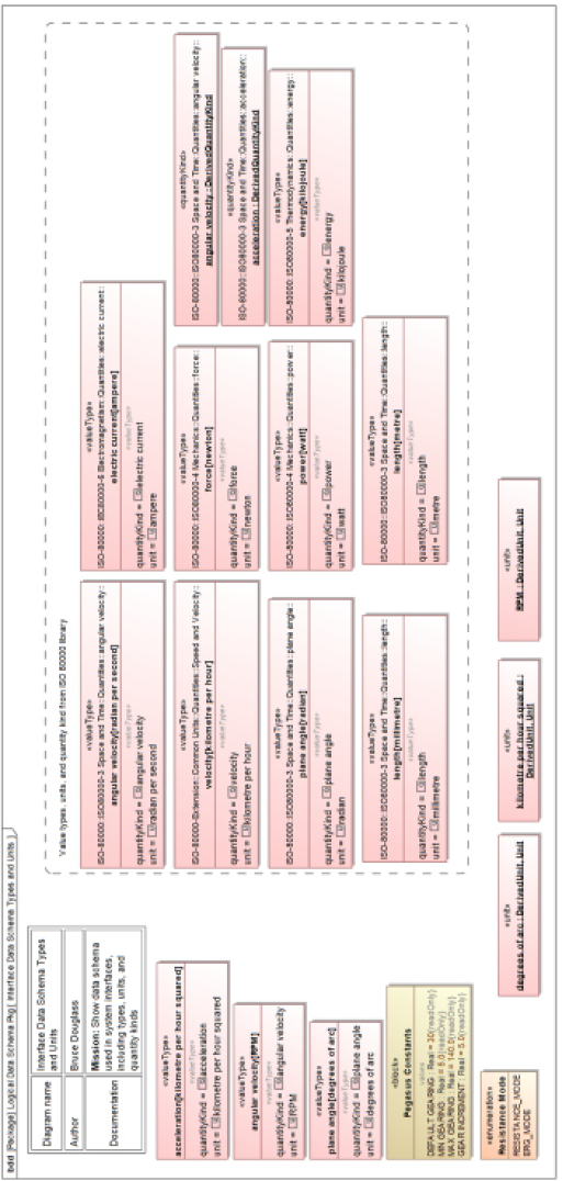
Figure 4.5: Scalar value types, units, and quantity kinds

Figure 4.6: Blocks and logical data schema

Preparation for Handoff

Purpose

The purpose of this recipe is to facilitate the handoff from systems engineering to downstream engineering. This will consist of a review of the handoff specifications for adequacy and organizing the information to ease the handoff activities. Ideally, each subsystem team needs access to system model information in specific and well-defined locations, and they only see information necessary for them to perform their work.

Inputs and preconditions

The precondition for this recipe is that the architecture is defined well enough to be handed off to subsystem teams for design and development. This means that:

• The system requirements for the handoff are stable and fit for purpose. This doesn’t necessarily mean that the requirements are complete, however. If an iterative development process is followed, the requirements need only be complete for the purpose of this increment.
• The subsystem architecture is defined including how it connects to other subsystems and the system actors. As in the previous point, not all subsystems need to be specified, nor must the included subsystems be fully specified in a given iteration for an incremental engineering process. It is enough that the subsystem architecture is specified well enough to meet the development needs of the current iteration.
• The subsystem requirements have been derived from the system requirements and allocated to the subsystems.
• The logical subsystem interfaces are defined so that the subsystems can collectively meet the system needs. This includes not only the logical specification of the services but also the logical data schema for the information those services carry. In addition, flows not directly related to services must also be logically defined as a part of the subsystem interfaces.

Outputs and postconditions

The resulting condition of the model is that it is organized well to facilitate the handoff workflows. Subsystem requirements and structures are accessible from external models with minimal interaction between the system and subsystem models.

How to do it

Figure 4.7 shows the workflow to prepare the handoff. While straightforward, doing a good job at this task means that the subsequent work for the handoff will be much easier:

Organize the subsystems

The next recipe, Federating Models for Handoff, will create a model for each subsystem. Each subsystem should reach into the system model as efficiently as possible to retrieve its – and only its – specification details. This is not to hide information about other subsystems but is instead meant to simplify the process of retrieving specification information that it needs. We must organize each subsystem into its own package so that the subsystem team can add this package to their model to serve as their starting architectural specification.

Organize the requirements

At this point, all the requirements relevant to the current handoff should be allocated to the subsystems. This means that the subsystems have relations identifying the requirements they must meet. These may be either «allocate» or «satisfy» relations, owned by the subsystem blocks and targeting the appropriate subsystems. This step involves locating the requirements so that they can be usably accessed by the downstream engineers and provided in summary views (tables and matrices). The package holding the requirements, which might be organized into subpackages, will be referenced by the individual subsystem models during and after the handoff.

Organize the interface data

One of the things put into the Shared Model (in recipes later in this chapter) is the physical interface specifications and the physical data schema for the data used within those interfaces. The logical interfaces and related schema must be organized within the systems engineering model so that it can easily be referenced by the Shared Model. This means putting the interfaces, interface blocks, and data definition elements – such as blocks, value types, quantity kinds, and units – in a package so that the Shared Model can easily reference it.

Review model for handoff readiness

After all the information is readied, it should be reviewed for completeness, correctness, and appropriateness for the downstream handoff workflow to occur. Participants in the review should be not only the systems engineers creating the information but also the subsystem engineers responsible for accepting it.

To review the readiness of the systems model for handoff, we look at the parts of the model that participate in the process:

• Subsystems:
  • Are the subsystems each nestled within their own packages?
  • Does each subsystem have ports defined with correct interfaces or interface blocks and with the proper conjugation?
  • Is the set of all subsystems complete with respect to the purpose of the handoff (e.g. does it support the functionality required of this specific iteration)?
  • Does each subsystem package have a reference to the requirements allocated to it?
• Requirements:
  • Are the requirements all located within a single package (with possible subpackages) for reference?
  • Are all requirements relevant to this handoff either directly allocated to subsystems or decomposed and their derived requirements allocated?
• Interfaces:
  • Is all the interface data located within a single package (which may have subpackages)?
  • Are all the interfaces or interface blocks detailed with the flow properties, operations, and event receptions?
  • Is the directionality of each interface feature set properly?
  • Are the properties of the services (operations and event receptions) complete, including data passed via those services?
  • Is the logical interface data schema fully, properly, and consistently defined for blocks, value types, quantity kinds, and units?

Example

The starting point for the example of this recipe is the detail shown at the front of this chapter. In this recipe, we will organize and refactor this information to facilitate the other handoff activities.

Organize the subsystems

Here, we will create a package within the Architecture Pkg::Architectural Design Pkg for each subsystem and relocate the subsystem block into that package. This will support later import into the subsystem model. These packages will be nested within the Architecture Pkg::Architectural Design Pkg. See Figure 4.8:

Figure 4.8: Subsystem organization in the system model

Organize the requirements

The requirements are held within the Requirements Analysis Pkg :: Requirements Pkg. While it is possible to redistribute the requirements into a package per subsystem based on those relations, it isn’t always practical to do so. Minimally, two summary views are needed. First, a table of the requirements showing the name and specification text of all requirements must be provided. This should be placed in the Requirements Analysis Pkg::Requirements Pkg so the subsystem teams can access it easily (as shown in Figure 4.2 and Figure 4.3) and use it to determine their requirements.

Secondly, matrix views showing the allocation relations between the subsystems and the allocated requirements are needed (as shown in Figure 4.3). Since the subsystems are the owners of the «allocate» and «satisfy» relations, it makes sense for these matrices to be in the Architecture Pkg::Architectural Design Pkg. The overall matrix can be put in that package directly. Figure 4.9 shows the package organization of the requirements in the model:

Figure 4.9: Requirements organization

In addition, each subsystem package contains an allocation matrix just showing the requirements allocated to that specific subsystem. Figure 4.10 shows the example for the Comms subsystem. The Cameo feature Show Elements > With relations is used to just show the requirements allocated to the Comms subsystem:

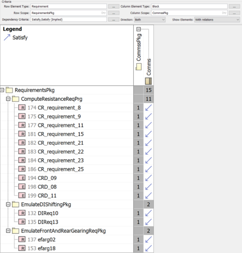
Figure 4.10: Comms subsystem allocated requirements

Organize the interface data

In the canonical model organization used in the example, the logical interfaces are located in the systems engineering model InterfacesPkg. These may be either Interfaces or Interface Blocks depending on whether standard or proxy ports are used. In addition, the package contains the specifications of the logical data passed via those interfaces, whether that data is expressed as service-independent flow properties or arguments for services. All this information should be organized for reference by the Shared Model, defined in the next recipe. The Shared Model will define physical interfaces and an associated data schema that represents the logical interfaces and data schema in the systems model. Those physical interfaces will then be made available to the subsystem teams via the model federation defined in the next recipe.

The information for this example is already shown in Figure 4.4, Figure 4.5 and Figure 4.6. The organization of the interface data is shown in Figure 4.11. Although the figure only shows the services for a single interface block, note that we have followed the convention of using event receptions for all logical service specifications in the systems engineering model. These will be changed into a physical schema in later recipes in this chapter:

Figure 4.11: Organization of interface data

Review model for handoff readiness

In this example, the model is set up and ready for handoff. See the Effective Reviews and Walkthroughs recipe in Chapter 5, Demonstration of Meeting Needs, for the workflow for performing the review.

Federating Models for Handoff

In SysML, a model is not the same as a project. A model is a special kind of package used to organize information for a particular modeling purpose. It may contain many nested packages and even other nested models. What we normally call the “systems engineering model” normally contains at least two models: a specification model (containing requirements, use cases, and functional analyses) and an architecture model (identifying subsystems and their properties, relations, and interfaces). There may be additional models for various analyses, such as trade studies or safety analyses.

In many cases, all these models are contained within a single SysML project. A project can contain one or more models, but a model can also be split across multiple projects. This is often done when the model is being worked on by different, geographically distributed teams. Projects and models are related but are distinct concepts. Many people just squint and say model = project and while that isn’t wrong, neither is it the entire story.

Downstream engineering is different in that many separate, independent models will be created. These models will interact with each other in specific and well-defined ways. A set of such independent, yet connected models is called a federation, and the process of creating the models and their linkages is called a model federation.

One of the key ideas in a model federation is the notion of a single source of truth. This concept means that while there may be multiple sources for engineering data, each specific datum is situated in a single, well-defined location known as the datum’s authoritative source. When a value is needed, the authoritative source for that data is referenced.

This means that, for the most part, data is not copied from model to model, which can lead to questions such as “The value reported for this datum is different if I look at different sources – so which is correct?” Instead, data is referenced.

To share packages from a project in Cameo, the source project must identify the packages allowed to be shared. This is done by right-clicking a package in the Cameo containment tree and selecting Project Usages > Share Packages. This pops up the Share Packages dialog, which allows the user to select which packages they will allow to be shared with other projects.

Sharing packages is how models are federated.

In the Cameo tool, model federations are constructed with the File > Use Project > Use Local Project feature (or File > Use Project > Use Server Project for projects stored on Teamwork Cloud). This feature can add data – usually packages with their contained elements – to other models. This feature loads in packages and model elements from other models or projects, provided they have been designated by that project owner as sharable. Once the Use Project dialog pops up, you can select the desired reference project and see the sharable packages. You can access them as read-only or read-write. In the former case, you can see the used model elements and create references to them. In the latter case, you can also create bidirectional relations with those elements and modify them – this can lead to synchronization issues later, so we recommend:

Always make packages in a federation read-only.

If the element in the source project must be changed, simply open the source project and make the edits.

While many models might be federated, including CAD models, PID control models, environment simulation models, and implementation models, we will focus on a core set of models in the recipe. The models in our federation will be:

• Systems engineering model:
  • This is the model we’ve been working with so far
• Shared Model:
  • This model contains elements used by more than one subsystem model
  • Our focus here will be the system and subsystem physical interfaces, including the physical data schema for information passed in those interfaces
• Subsystem model [*]:
  • A separate model per subsystem is created to hold its detailed design and implementation

Purpose

The purpose of this recipe is to provide workspaces to support both the handoff process itself and the downstream engineering work to follow.

Inputs and preconditions

The starting point for this recipe is the system engineering model with engineering data necessary to perform the handoff to downstream engineering, including the set of identified subsystems. This information is expected to be organized to facilitate the referencing of requirements, architectural elements, and interface data for the linking together of the models in the federation.

Outputs and postconditions

At the end of the recipe, a set of models are constructed with limited and well-defined points of interaction. Each model is created with a standard canonical model organization supportive of its purpose.

How to do it

The steps involved in the recipe are shown in Figure 4.12:

Figure 4.12: Create model federation

Create the Shared Model

Create a new model, named the Shared Model. This is normally located in a folder tree underneath the folder containing the system engineering model, but it needn’t necessarily be so.

Structure the Shared Model

This model has a recommended initial structure containing the package Physical Interfaces Pkg, which will be referenced by the Subsystem Models. This package will hold the specification of the interfaces and has two nested packages, one for the physical data schema and the other for related stereotypes. The stereotypes are commonly used to specify metadata to indicate subranges, extent, and precision, and this information is important for the subsystem teams to use those data successfully. The subsystems need a common definition for interfaces and they get it by referencing this package.

It should be noted that it is common to add an additional DomainsPkg later in the downstream engineering process to hold design elements common to multiple subsystems, but the identification of such elements is beyond the scope of the handoff activity.

Add SE Model references to the Shared Model

There are a small number of SE Model packages that must be referenced in the Shared Model. Notably, this includes:

• A Requirements Pkg package
• An Interfaces Pkg package
• A Shared Common Pkg package, which may contain a Common Stereotypes profile

The first two are discussed in some detail in the previous recipe. The Shared Common package includes stereotypes and other reusable elements that may be necessary to properly interpret the elements in the referenced packages.

In Cameo, adding these references is done with the File > Use Project feature. If you select the menu item, the Use Project dialog will open and you can navigate to the systems engineering model you want to reference.

Once there, you can select the packages it has shared (Figure 4.13):

Figure 4.13: Use Project dialog

It is highly recommended that you use the packages as Read-only. This will prevent synchronization problems later. If you need to modify the source package, open up the system engineering model and edit it there.

Create the subsystem model

It is assumed that each subsystem is a well-defined, mostly independent entity and will generally be developed by a separate interdisciplinary engineering team. For this reason, each subsystem will be further developed in its own model. In this step, a separate model is created for the subsystem.

This step is repeated for each subsystem.

Structure the subsystem model

A standard canonical structure is created for the subsystem. It consists of two packages, although it is expected that the subsystem team will elaborate on the package structure during the design and implementation of that subsystem. These packages are:

• A Subsystem Spec Pkg package:
  • This package is intended to hold any requirements and requirements analysis elements the team finds necessary. Further recipes will discuss the creation of refined requirements for the included engineering disciplines and their facets.
• A Deployment Pkg package:
  • This package contains what is known as the deployment architecture for the subsystem. This is a creation of engineering-discipline-specific facets, which are contributions to the subsystem design from a single engineering discipline. The responsibilities and connections of these facets define the deployment architecture.

This step is repeated for each subsystem.

Add SE Model references to the subsystem model

Each subsystem model has two important references in the SE Model:

• Subsystem package:
  • In the previous recipe, each subsystem was located in its own package in the SE Model, along with its properties and a matrix identifying the requirements it must meet. The package has the original name of the subsystem package in the SE Model.
• Requirements Pkg package:
  • This is a reference to the entire set of requirements, but the matrix in the subsystem package identifies which of those requirements are relevant to the design of the subsystem.

While in almost all cases, it is preferable to add these other model packages to the subsystem model by reference, it is common to add the subsystem package by value (copy). The reason is that in an iterative development process, systems engineering will continue to modify the SE Model for the next iteration while the downstream engineering teams are elaborating the subsystem design for the current iteration. As such, the subsystem teams don’t want to see new updates to their specification model until the next iteration. By adding the subsystem spec package by copy, it can be updated at a time of the subsystem teams choosing and SE Model updates won’t be reflected in the subsystem model until the subsystem model explicitly updates the reference. Any relations from other subsystem model elements to the elements in the subsystem spec package will be automatically updated because the reloaded elements will retain the same GUID. However, any changes made to the copied elements will be lost.

Insulation from changes made by system engineers can also be handled by a configuration management tool that manages baselined versions of the referenced models, so there are multiple potential solutions to this issue.

This step is repeated for each subsystem.

Add Shared Model references to the subsystem model

The relevant package to reference in the Shared Model is Physical Interfaces Pkg. This will contain the interface definitions and related data used by the subsystems, including the physical data schema.

This step is repeated for each subsystem.

Example

In this example, we will be creating a Shared Model and a subsystem model for subsystems Comms, Electrical Power Delivery, Main Computing Platform, Mechanical Frame, Power Train, and Rider Interaction.

Create the Shared Model

We will put all these models, including the Shared Model, in a folder located in the folder containing the SE Model. This folder is named Subsystem Model and contains a nested folder, SharedModel.

Structure the Shared Model

It is straightforward to add Physical Interfaces Pkg and its nested packages.

Add SE Model references to the Shared Model

It is similarly straightforward to add the references back to the common, requirements, and logical interface packages in the systems engineering model. When this step is complete, the initial structure is as shown in Figure 4.14. The grayed-out package names are the shared/referenced packages from the systems engineering model and the darker package names are the ones that are new and owned by the Shared Model:

Figure 4.14: Initial structure of the Shared Model

Create the subsystem model

For every subsystem, we will create a separate subsystem model. If we are practicing incremental or agile development, the handoff recipes will be performed multiple times during the project. In this case, it isn’t necessary that all of the subsystem will be involved in every increment of the system, so subsystem models only need to be created for the subsystems that participate in the current iteration.

In this example, those subsystems are Comms, Electric Power Delivery, Main Computing Platform, Mechanical Frame, Power Train, and Rider Interaction.

Structure the subsystem model

Although the subsystem models may evolve differently depending on the needs and engineering disciplines involved, they all start life with a common structure. This structure consists of a Subsystem Spec Pkg and Deployment Pkg packages. If software engineering is involved in subsystem development, then additional packages to support software development are added as well. While it’s not strictly a part of the handoff activity per se, I’ve added a typical initial structure for software development in the Main Computing Platform model, shown in Figure 4.15.

Add SE Model references to the subsystem model

Each subsystem model must have access to its specification from the SE Model; as previously mentioned this can be done by value (copy) or by reference (project usage). In the previous recipe, we organized the SE Model to simplify this step; the information for a specific subsystem is all located in one package nested within the Architecture Design Pkg. In our example SE Model, the names of these subsystem packages are simply the name of the subsystem followed by the suffix Pkg. For example, the package containing the Main Computing Platform subsystem is Main Computing Platform Pkg.

In addition, each subsystem model must reference the Requirements Pkg package so that it can easily locate the requirements it must satisfy.

Add Shared Model references to the subsystem model

Finally, each subsystem needs to reference the common physical interface specifications held in the Shared Model:

Figure 4.15: Main computing subsystem model organization

Logical to Physical Interfaces

The previous chapters develop interfaces from the functional analysis (Chapter 2, System Specification) and the architecture (Chapter 3, Developing Systems Architecture). These are all logical interfaces that are defined by a set of logical services or flows. These logical interfaces characterize their logical properties – extent, precision, timeliness, and so on – as metadata on those features. In this book, all services in the logical interface are represented as events that possibly carry information or as flow properties. In this recipe, that information is elaborated in a physical data schema, refining their physical properties.

The subsystem teams need physical interface specifications, since they are designing and implementing physical systems that will connect in the real world. We must refine the logical interfaces to include their implementation detail – including the physical realization of the data – so that the subsystems can be properly designed and be ensured to properly connect and collaborate in actual use.

For example, a logical service specifying a command to enter into configuration mode such as evSetMode(CONFIGURATION_MODE) might be established between an actor, such as the Configuration App, and the system. The physical interface might be implemented as a Bluetooth message carrying the commanded mode in a specific bit format. The bit format for the message that sends the command is the physical realization of the logical service.

A common system engineering work product is an Interface Control Document (ICD). While I am loath to create a document per se, the goal itself is laudable – create a specification of the system interfaces and their metadata and present it in a way that can be used by a variety of stakeholders. I talk about creating model-based ICDs both on my website (https://www.bruce-douglass.com/_files/ugd/21dc4f_7bf30517b9ca46c59c21eddedf18663c.pdf) and on my YouTube channel (https://www.youtube.com/watch?v=9pzjMkhFIoM&t=23s). What should an ICD contain?

An ICD should identify:

• Systems and their connections and connection points
• Interfaces, which in turn contain:
  • Service specifications, including:
    • Service name
    • Service parameters, including their direction (in, out, or inout)
    • Service direction (e.g. provided vs required)
    • Description of functionality
    • Preconditions, post-conditions, constraints, and invariants
  • Flow specifications, including:
    • Flow type
  • Data schema for arguments and flows:
    • Type model
    • Metadata, including extent (set of valid values), precision, accuracy, fidelity, timeliness, and other constraints

In SysML models, this means that the primary element will be Interface Blocks and their owned features.

Representing an ICD

In SysML, ICD can be visualized as a set of diagrams, tables, matrices, or (in a best case scenario) a combination of all three. One of the useful mission types for block definition diagrams that I use is creating an Interface Diagram, which is nothing other than a BDD whose purpose is to visualize some set of interfaces, their owned features, and related metadata. I normally create one such diagram for each subsystem, showing the ports and all the interfaces specifying those ports. It is also easy to create an Interface Specification Table (in Cameo, usage of a Generic Table) that exposes the same information but in tabular form. An advantage of the tabular format is the ease with which the information can be exported to spreadsheets.

Purpose

The purpose of this recipe is to create physical interfaces and physical data schema and store them in the Shared Model so that subsystem teams have a single source of truth for the definition of actor, system, and subsystem interfaces.

Note that any interfaces defined within a subsystem are out of scope for this recipe and for the Shared Model; this recipe only addresses interfaces between subsystems, the system, and the actors, or between the subsystems and the actors.

Inputs and preconditions

The inputs for the recipe include the logical interfaces and the logical data schema. Preconditions include the construction of the Shared Model complete with references to the logical interfaces and data schema in the SE Model.

Outputs and postconditions

The outputs from this recipe include both the physical interface specifications and the physical data schema organized for easy import into the subsystem models.

How to do it

The workflow for the recipe is shown in Figure 4.16:

Figure 4.16: Define physical interfaces

Reference the logical interfaces

The physical interfaces we create must satisfy the needs of the already-defined logical interfaces. To start this recipe, we must review and understand the logical interfaces.

Select technology for physical interfaces

Different technological solutions are available for the implementation of physical interfaces. Even for something like a mechanical power transfer interface, different solutions are possible, such as friction, gearing, direct drive, and so on. For electronic interfaces, voltage, wattage, amperage, and phase must be specified. However, software interfaces – or combined electro-software interfaces – are where most of the interface complexity of modern systems reside.

In the previous recipes, we specified a logical interface using a combination of flow properties (mostly for mechanical and electronic interfaces) and signal events (for discrete and software interfaces). This frees us from early concern over technical detail while allowing us to specify the intent and logical content of interfaces. Once we are ready to direct the downstream subsystem teams this missing detail must be added.

Flow properties with mechanical or electronic realization may be implemented as energy or matter flows, or – if informational in nature – perhaps using a software middleware such as Data Distribution Service (DDS). Events are often implemented as direct software interfaces or as messages using a communication protocol.

The latter case is an electro-software interface, but the electronics aspect is dictated by a standard in the physical layer of the protocol definition and while the software messages are constrained by the defined upper layers of the protocol stack. This is assuming that your realization uses a pre-defined communications standard. If you define your own, then you get the joy of specifying those details for your system.

In many cases, the selection of interface technology will be driven by external systems that already exist; in such cases, you must often select from technology solutions those external systems already provide. In other cases, the selection will involve performing trade studies (see the Architectural Trade Studies recipe from the previous chapter) to determine the best technical solutions.

Select technology for use interfaces

User interfaces (UIs) are a special case for interface definition. Logical interfaces defining UIs are virtual in the sense that our system will not be sending flows or services directly to the human user. Instead, a UI provides sensors and actuators manipulated or used by human users to provide the information specified in the logical interfaces. These sensors and actuators are part of the system design. Inputs from users in a UI may be via touchscreens, keyboards, buttons, motion sensors, or other such devices. Outputs are perceivable by one or more human sensors, typically vision, hearing, or touch. The interactions required of the UI are often defined by a human factors group that does interaction workflow analysis to determine how users should best interact with the system. The physical UI specification details the externally-accessible interactions although not necessarily the internal technical detail. For example, the human factors group may determine that selection buttons should be used for inputs and small displays for output, but the subsystem design team may be charged with the responsibility of selecting the specific kind of buttons (membrane vs tactile) and displays (LED, LCD, plasma, or CRT).

Define the physical realization of the logical interfaces

Once the technology of the physical interfaces is decided, the use of the technology for the interfaces must be defined. This is straightforward for most mechanical and electronic interfaces, but many choices might exist for software. For example, TCP/IP might be a selected technology choice to support an interface. The electronic interfaces are well defined in the physical layer specification. However, the software messages at the application layer of the protocol are defined in terms of datagrams. The interfaces must define the internal structuring of information within the datagram structure.

The basic approach here is to define the message packet or datagram internal data structure, including message identifier and data fields, so that the different subsystems sending or receiving the messages can properly create or interpret the messages. Be sure to add a dependency relation from the physical packet or datagram structure to the logical service being realized. I create a stereotype of dependency named «represents» for this purpose. The relations can best be visualized in matrix form.

Add «represents» relations

It is a good idea to add navigable links from the physical interfaces back to their logical counterparts. This can be done as a «trace» relation, but I prefer to add a stereotype just for this purpose named «represents». I believe this adds clarity whenever you have model elements representing the same thing at different levels of abstraction. The important thing is that from the logical interface, I can identify how it is physically realized, and from the physical realization, I can locate its logical specification.

Create interface visualization

In this step, we create the diagrams, tables, and matrices that expose the interfaces and their properties to the stakeholders.

Example

In this example, we will focus on the logical interfaces shown in Figure 4.4. We will define the physical interfaces and physical ports.

Reference the logical interfaces

In the last recipe, we added the Interfaces Pkg from the SE Model for reference. This means that we can view the content of that package, but cannot change it in the Shared Model, only in the owning SE Model. The model reference allows use to create navigable relations from our physical schema to its logical counterpart.

Select technology for physical interfaces

The interfaces in Figure 4.4 have no flow properties so we must only concern ourselves with the event receptions of the interfaces. Specifically, the Configuration App and Training App communicate with the system via a Bluetooth Low Energy (BLE) wireless protocol. The system must also interact with its own sensors via either BLE or ANT+ protocols for heart rate and pedal data, but we are considering those interfaces to be internal to the subsystems themselves and so they will not be detailed here.

The BLE interfaces in our current scope of concern are limited to the Comm subsystem and the Configuration App and Training App.

For internal subsystem interfaces, different technologies are possible, including RS-232, RS-485, the Control Area Network (CAN) bus, and Ethernet. Once candidate solutions are identified, a trade study (not shown here but described in the previous chapter’s Architectural Trade Studies recipe) would be done and the best solution would be selected.

In this example, we select the CAN bus protocol. This technology will be set to connect all subsystems that are software services, such as the interfaces among the Comm, Main Computing Platform, Rider Interaction, and Power Train subsystems. The interactions for the Electric Power Delivery subsystem will be electronic digital signals. Table 4.1 summaries the technology choices:

Interface	Participants	Purpose	Technology
App Interface	Comm subsystem Training app Configuration app	Send Rider data to the Training app for display and analysis. Support system configuration by the Configuration app.	BLE
Pedal Interface	Rider Power Train subsystem	Reliably connect to Rider’s shoes via cleats in order to determine the power from the Rider in which position and cadence can be computed.	Look™ compatible clipless pedal fit Standard pedal spindle Pedal-based power meter
Internal Bus	Comms subsystem Rider Interaction subsystem Power Train subsystem Main Computing Platform subsystem Mechanical Frame subsystem	Send commands and data between subsystems for internal interaction and collaboration, including sending information to the Comms subsystem to send to the apps, and sending received information from the apps received by the Comms subsystem to other subsystems.	CAN bus
Power Enable	Power subsystem Rider Interaction subsystem Main Computing Platform subsystem	Signal the power system to turn power on and off.	Digital voltage 0-5V DC
Electrical Power	Electric Power Source Electrical Power Delivery subsystem	Electrical power provided from the external power source to the system	100-240V, 5A, 50-60Hz AC
Electrical Power distribution	Electric Power Delivery subsystem and: High Power: Power Train subsystem Medium Power: Mechanical Frame subsystem Digital Power: Rider Interaction subsystem Main Computing Platform subsystem Comms subsystem Power Train subsystem	Electrical power is transformed and delivered to subsystems in one of three ways: High power for the motor to generate resistance to pedaling for the Rider Medium power for the Mechanical Frame subsystem to raise or lower the incline Digital Power provided to the components using digital power	To be defined by the Electric Power Delivery subsystem team working with the other subsystem teams

Table 4.1: Interface technologies

Of these technologies, BLE and the CAN bus will require the most attention.

Select technology for UIs

There are several points of human interaction in this system that are not in the scope of this particular example handoff, including the mechanical points for fit adjustments, the seat, and the handlebars. In this particular example, we focus on the rider interface via the pedals, the gear shifters, the power button, and the gearing display. The rider metrics and ride performance are all displayed by the Training App while the Configuration App provides the UI for setting up gearing and other configuration values.

The Pegasus features a simple on-bike display for the currently selected gearing and current incline, mocked up in Figure 4.17. It is intended to be at the front of the bike, under the handlebars but in easy view of the Rider. It sports the power button, which is backlit when pressed, a gearing display, and the currently selected incline.

The gearing display will display the index of the gear selected, not the number of teeth in the gear:

Figure 4.17: On-bike display

To support Shimano and DI shifting emulation, each handlebar includes a brake lever that can be pressed inward to shift up or down for the bike (left side for the chain ring, right side for the rear cassette). In addition, the inside of the shifter has one button for shifting (left side for up, right side for down) to emulate Digital Indexed (DI) shifting.

Define the physical realization of the logical interfaces

Let’s focus on the messaging protocols as they will implement the bulk of the services. Bluetooth and its variant BLE are well-defined standards. It is anticipated that we will purchase a BLE protocol stack so we only need to be concerned about the structuring of the messages at the 1, that is, structuring the data within the Payload field of the Data Channel PDU (Figure 4.18):

Figure 4.18: BLE packet format

Similarly, for internal bus communication, the CAN bus protocol is well developed with commercial chipsets and protocol stacks available. The CAN bus is optimized for simple data messages and comes in two forms, one providing an 11-bit header and another a 29-bit header. The header defines the message identifier. Because the CAN bus is a bit-dominance protocol, the header also defines the message priority in the case of message transmission collisions. We will use the 29-bit header format so we needn’t worry about running out of message identifiers. In either case, the data field may contain up to 8 bytes of data, so that if an application message exceeds that limit, it must be decomposed into multiple CAN bus messages and reassembled at the receiver end. The basic structure of CAN bus messages is shown in Figure 4.19:

Figure 4.19: CAN bus message format

For CAN bus messages, we’ll use an enumeration for the message identifier and define the structure of the data field for interpretation by the system elements.

The basic approach taken is to create base classes for the BLE and CAN bus messages in the Shared Model. Each will have an ID field that is an enumeration of the message identifiers; it will be the first field in the BLE PDU. That is, the BLE messages that have no data payload will only contain the message ID field in the BLE message data PDU. The CAN bus messages will be slightly different; the ID field in the message type will be extracted and put into the 29-bit identifier field. Data-less messages will have no data in the CAN bus data fields but will at least have the message identifier.

We won’t show all the views of all the data elements, but Figure 4.20 shows the types for the BLE packets and physical data types:

Figure 4.20: Physical data schema for BLE messages

This figure merits a bit of discussion. First, this data schema denotes the physical schema for bits-over-the-air; this is not necessarily how the subsystem stores the data internally for its own use. Secondly, note that the figure denotes the use of some C++ language-specific types, such as uint_t as the basis for the corresponding transmission type uint_1Byte. Next, note the types scaled_int32x100 and scaled_int16x100. These take a floating-point value and represent them as scaled integers – in the former case, multiplying the value times 100 and storing it as a 32-bit signed integer, and in the latter case, multiplying the value times 100 and storing it in a 16-bit signed integer. The practice of using scaled integers is very common in embedded systems and cuts down on bandwidth when lots of data must be passed around. Metadata specified for the logical interfaces must be copied or added and refined in the physical interfaces.

For example, if the range of power applied by the Rider in the logical interface is specified to be in the subrange (0...2000) and units of watts, then this would need to be replicated in the physical data schema as well. Lastly, note how the physical data schema blocks have «represents» relations back to elements in the logical data schema (color-coded to show them more distinctly).

Figure 4.21 shows how these data elements are used to construct BLE packets. The logical data interface blocks for the Training App and Configuration App are shown in the upper part of the figure (again, with special coloring), along with their services. Each service must be represented by one of the defined packet structures. The structure of the BLE Packet class has a pdu part, of type PDU_Base. PDU_Base contains a 2-byte header, which indicates the message size as well as a msg_type attribute of type APP_MESSAGE_ID_TYPE, which is an enumeration of all possible messages. Messages without data, such as evClose_Session, can be sent with a BLE Packet with a pdu part of type PDU_Base.

For messages that carry data, PDU_Base is subclassed to add appropriate data fields to support the different messages, so that a BLE Packet can be constructed with an appropriate subtype of the PDU_Base to carry the message data. For example, to send the logical message evReqSetGearConfiguration, the BLE Packet would use the PDU_Gearing subclass of PDU_Base:

Figure 4.21: BLE Packets

While messages between the system and the apps use Bluetooth, messages between subsystems use an internal CAN bus. The CAN bus physical schema is different in that it must be detailed to the bit level, since there are packet fields of 1, 4, 7, 11, and 18 bits in addition to elements of one or more byte lengths. We’ll let the software engineers define the bit-level of the manipulation of the fields and just note, by type, those fields that have special bit lengths where necessary. Figure 4.22 shows the structure of the CAN bus messages that correspond to the services:

Figure 4.22: CAN bus messages

Add «represents» relations

We must add the «represents» relations so it is clear which Bluetooth or CAN bus messages are used to represent which logical services in the SE Model interface blocks.

These relations are best visualized in a matrix. We will define a matrix layout that uses the following settings:

• From Element Types: Block
• To Element Types: Receptions
• Cell Element Types: Represents the stereotype of dependency

Then we can use that matrix layout to create a matrix view (created in Cameo as a “dependency matrix”) with the Physical Interfaces Pkg set to the From Scope and Interfaces Pkg referenced from the SE Model.

When you’re all done, you should have a matrix of the relations from the messaging classes to the event receptions in the SE Model interface blocks, as shown in Figure 4.23:

Figure 4.23: Message mapping to logical services

Create interfaces visualization

In this step, we want to create a model-based version of an Interface Control Document (ICD).

In this example, I will show a subsystem interface diagram (Figure 4.24) and an interface specification table (Figure 4.25). In a real project, I would create a subsystem interface diagram for every subsystem in the project increment and the table would be fully elaborated:

Figure 4.24: Subsystem interface diagram

Figure 4.25: Interface specification table

Deployment Architecture I: Allocation to Engineering Facets

The Federating Models for Handoff recipe created a set of models: a Shared Model and a separate model per subsystem. The current recipe creates what is called the deployment architecture and allocates subsystem features and requirements to different engineering disciplines. Once that is done, the real job of software, electronic, and mechanical design can begin, post-handoff. In this chapter, we will separate two key aspects of the deployment architecture into different recipes. The first will deal with the allocation of subsystem features to engineering facets. The next recipe will focus on the definition of interdisciplinary interfaces enabling those facets to collaborate.

Deployment architecture

Chapter 3, Developing Systems Architecture, began with a discussion of the “Six Critical Views of Architecture.” One of these – the Deployment Architecture – is the focus of this and the next recipes. The deployment architecture is based on the notion of facets. A facet is a contribution to a design that comes from a single engineering discipline (Figure 4.26). We will not design the internal structure or behavior of these facets, but will refer to them collectively; thus, we will not identify here software components, or electrical parts, but rather simply refer to all the contributions from these as the “software facet” or “electronics facet.” A typical subsystem integrates a number of different facets, the output from engineering in disciplines such as:

• Electronics:
  • Power electronics
  • Motor electronics
  • Analog electronics
  • Digital electronics
• Mechanics:
  • Thermodynamics
  • Materials
  • Structural mechanics
  • Pneumatics
  • Hydraulics
  • Aerodynamics
  • Hydrodynamics
• Optics
• Acoustics
• Chemical engineering
• Software:
  • Control software
  • Web/cloud software
  • Communications
  • Machine learning
  • Data management

Figure 4.26: Some engineering facets

These disciplines may result in facets at a high-level of abstraction – such as an electronics facet – or may result in more detailed facets – such as power, motor, and digital electronics, depending on the needs and complexity of the subsystem.

A subsystem team is generally comprised of multiple engineers of each discipline working both independently on their aspect of the design and collaboratively to produce an integrated, functioning subsystem.

Creating a deployment architecture identifies and characterizes the facets and their responsibilities in the scope of the subsystem design. This means that the subsystem features – subsystem functions, information, services, and requirements – must be allocated to the facets.

This makes it clear to the subsystem discipline-specific engineers what they need to design and how it contributes to the overall subsystem functionality.

The deployment architecture definition is best led by a system engineer but must include input and contributions from discipline-specific engineers to carry it forward. This is often called an Interdisciplinary Product Team (IPT). Historically, a common cause of project failure is for a single engineering discipline to be responsible for the creation of the deployment architecture and allocation of responsibilities. Practice clearly demonstrates that an IPT is a better way.

The system engineering role in the deployment architecture is crucial because system engineers seek to optimize the system as a whole against a set of product-level constraints. Nevertheless, it is a mistake for systems engineers to create and allocate responsibilities without consulting the downstream engineers responsible for detailed design and implementation. It is also a (common) mistake to let one discipline make the deployment decisions without adequate input from the others. I’ve seen this on many projects, where the electronics designers dictate the deployment architecture and end up with a horrid software design because they didn’t adequately consider the needs of the software team. It is best for the engineers to collaborate on the deployment decisions, and in my experience, this results in a superior overall design.

Purpose

The purpose of this recipe is to create the deployment architecture and allocate subsystem features and requirements to enable the creation of the electronic, mechanical, and software design.

Inputs and preconditions

The preconditions are that the subsystem architecture has been defined, subsystems have been identified, and system features and requirements have been allocated to the subsystems.

Inputs include the subsystem requirements and system features – notably system data, system services, and system functions – that have been allocated to the subsystem.

Outputs and postconditions

The output of this recipe is the defined deployment architecture, identified subsystem facets, and allocation of system features to those facets.

The output is the updated subsystem model with those elements identified and allocated.

How to do it

Figure 4.27 shows the recipe workflow. This recipe is similar to the Architectural Allocation recipe in Chapter 3, Developing Systems Architecture, except that it focuses on the facets within a subsystem rather than on the subsystems themselves. This recipe is best led by a system engineer but performed by an interdisciplinary product team to optimize the deployment architecture:

Figure 4.27: Create the deployment architecture

Identify contributing engineering facets

The first step of the recipe is to identify the engineering disciplines involved. Some subsystems might be mechanical only, electrical-mechanical, software-electronic, or virtually any other combination. Any involved engineering discipline must be represented so that their facet contribution can be adequately characterized. For an embedded system, a software-centric subsystem typically also includes electronic computing infrastructure (a digital electronic facet) to provide hardware services to support the functionality. The capacities of the electronics facet, including memory size, CPU throughput, and so on, are left to negotiation among the coordinating engineering disciplines.

This topic is discussed in a bit more detail in the next recipe, Deployment Architecture II: Interdisciplinary Interfaces.

Create a block for each facet

In the deployment model, we will create a block for each facet. We will not, in general, decompose the facet to identify its internal structure. That is a job for discipline-specific engineers who have highly developed skills in their respective subject matters. It is enough, generally, to create a separate block for each facet. Each facet block will serve as a container or collector of specification information about that facet for the downstream engineering work.

Decompose non-allocatable requirements

Requirements can sometimes be directly allocated to a specific facet. In other cases, it is necessary to create derived requirements that take into account the original subsystem requirements and the specifics of the subsystem deployment architecture. In this latter case, create derived requirements that can be directly allocated to subsystems. Be sure to add «deriveReqt» relations from the derived requirements back to their source subsystem requirements. These derived requirements can either be stored in the subsystem model, the system model, or in a requirements management tool, such as IBM DOORS™.

Allocate requirements to facets

Allocate system requirements to the identified facets. In general, each requirement is allocated to a single facet, so in the end, the requirements allocated to the subsystem are clearly and unambiguously allocated to facets. The set of allocated subsystem requirements after this step is normally known as software, electronic, or mechanical requirements. It is crucial that the engineers of the involved disciplines are a part of the allocation process.

Decompose non-allocatable subsystem features

Some subsystem features – which refer to operations, signal receptions, flows, and data – can be directly allocated to a single facet. In practice, most cannot. When this is the case, the feature must be decomposed into engineering-specific-level features that trace back to their subsystem-level source feature but can be directly allocated to a single facet.

Allocate subsystem features to facets

Each subsystem function now becomes a service allocated to a single facet OR it is decomposed to a set of services, each of which is so allocated. Subsystem flows and data must also be allocated to facets as well.

Perform initial facet load analysis

This step seeks to broadly characterize the size, capacity, and other summary quantitative properties of the facets. The term load means different things in different disciplines. For mechanical facets, it might refer to weight or shear force. For digital electronics, it might refer to CPU throughput and memory size. For power electronics, it might mean the maximum available current. For software, it might mean volume (roughly, “lines of code”), nonvolatile storage needs, volatile memory needs, or message throughput. The important properties will also differ depending on the nature of the system. Helicopters, for example, are notoriously weight-sensitive, while automobiles are notoriously component price-sensitive (meaning they want to use the smallest CPUS and the least memory possible). These system characteristics will drive the need for the quantification of different system properties.

These properties will be estimates of the final product qualities but will be used to drive engineering decisions. Digital electronics engineers will need to design or select CPU and memory hardware, and they need a rough guess of the needs or requirements of the software to do so. It is far too common that a lack of understanding leads to the design of underpowered computing hardware resulting in decreased software (and therefore, system) performance. Is a 16-bit processor adequate or does the system need a pair of them or a 32-bit CPU? Is 100Kb of memory adequate or does the system need 10Mb? Given these rough estimates, downstream design refines and implements these properties.

Estimating the required capacity of the computing environment is difficult to do well and a detailed discussion is beyond the scope of this book. However, it makes sense to introduce the topic and illustrate how it might be applied in this example. Let’s consider memory sizing first.

Embedded systems memory comes in several different kinds, each of which must be accessible by the software (i.e. part of the software “memory map”). Without considering the underlying technology, the kinds of memory required by embedded software are:

• Non-reprogrammable non-volatile memory:

This kind of memory provides storage for code that can never be changed after manufacturing. It provides boot-loading code and at least low-level operating system code.

• Programmable non-volatile memory:

This kind of memory provides storage for software object code and data that is to be retained across power resets. This can be updated and rewritten by program execution or via Over-the-Air (OTA) updates.

• Programmable read-write memory for software object code execution:

Because of the relatively slow access times for non-volatile memory, it is not uncommon to copy software object code into normal RAM for execution. Normally, the contents of this memory are lost during power resets.

• Programmable read-write memory for software data (heap, stack, and global storage):

This memory provides volatile storage for variables and software data during execution. Generally, the contents of this memory are lost during power resets.

• Electronic registers (“pseudo-memory”):

This isn’t really memory, per se, as it refers to hardware read-only, write-only, and read-write registers used to interface between the software and the digital electronics.

• Interrupt vector table:

This isn’t a different kind of memory as it may be implemented in any of the above means but must be part of the memory map.

A typical approach is to estimate the need for each of the above kinds of memory and then construct a memory map, assigning blocks of addresses to the kinds of memory. It is common to then add a percentage beyond the estimated need to provide room to grow in the future.

CPU capacity can be measured in many ways. CPU capacity estimating can be performed by comparing the computation expectations of a new system based on throughput measurements of existing systems. An alternative is to base it on experimentation: write a “representative” portion of the software, run it on the proposed hardware platform, measure the execution time, bandwidth or throughput, and then scale it to your estimated software size. You can even do “cycle counting” by determining the CPU cycles needed to perform critical functionality on a given CPU, and then compute the CPU speed as a cycle rate fast enough to deliver the necessary functionality within the timeliness requirements. Of course, there are many other considerations that go into a CPU decision including cost, availability, longevity, and development support infrastructure.

Example

We will limit our example to a single subsystem identified in the last chapter: the Power Train subsystem.

Identify contributing engineering facets

The Power Train subsystem is envisioned to have mechanical, electronic, and software aspects.

Create a block for each facet

Figure 4.28 shows the blocks representing these facets while Figure 4.29 shows how they connect. Note the «software», «electronics», and «mechanical» stereotypes added to the facet blocks. I defined these stereotypes in the Shared Model::Shared Common Pkg package so that they are available to all subsystems. This is an example of the use of stereotypes to indicate a “special kind of” modeling element.

Also note the connection points for those facets. There are two pairs of ports between the Software and Electronics blocks, one for communications (it is anticipated that the electronics will provide an interface to the CAN bus) and one for interaction with the electronics of the power train. This separation is not a constraint on either the software or electronics design but represents the connections between the facets being really independent of each other.

There is both a port pair and an association between the Electronic and Mechanical blocks on the BDD and a corresponding connector between their instances on the IBD. This is a personal choice of how I like to separate dynamic and static connections between these facets by modeling them with ports and direct associations, respectively. By dynamic, I am referring to connections that convey information or flows during system operation.

By static, I am referring to connections that do not, such as the physical attachments of electronic components to the mechanical power train with bolts or screws:

Figure 4.28: Deployment Architecture BDD

Figure 4.29: Connected deployment architecture IBD

Decompose non-allocatable requirements

These facets provide responsible elements to which requirements may be allocated. As mentioned, many requirements must be decomposed into derived requirements prior to allocation.

One issue is where to place such requirements. If you are using a third-party requirements management tool such as DOORS, then clearly, this tool should hold those requirements. If you are instead managing the requirements directly in your model, then there are a couple of options: the Requirements Pkg package in the SE Model or in the subsystem model. I personally prefer the latter, but valid arguments can be made for the former. In this case, I will create a Capabilities::Requirements Pkg package inside the Power Train Subsystem Model to hold these requirements.

Before we can decompose requirements for this subsystem, we need to highlight the relevant requirements, i.e. the ones to which the Power Train subsystem has an «allocate» or «satisfy» relation. The Power Train Pkg, imported from the SE Model, has these relations, and the Requirements Pkg, also loaded from the SE Model, has the requirements. The appropriate requirement may be easily identified by creating a relation map in Cameo for the Power Train block (right-click the block and select Related elements > Create Relation Map) or by building a matrix. Both are shown in Figure 4.30:

Figure 4.30: Finding requirements allocated to the subsystem

Having identified the relevant requirements, it is a simple matter to build a requirements diagram exposing just those requirements in the Subsystem Requirements Pkg package (Figure 4.31):

Figure 4.31: Requirements allocated to the power train subsystem

When working in diagrams, adding derived requirements is straightforward. For example, look at Figure 4.32. In this figure, which works with a subset of the subsystem requirements, we see the facet requirements with «deriveReqt» relations. I’ve also added the facet stereotypes to clarify the kind of requirement being stated:

Figure 4.32: Diagrammatically adding facet requirements

The other subsystem requirements are decomposed in other requirements diagrams. The derived requirements are summarized in Table 4.2:

Requirement Name	Specification	Derived From
EEReq_01	The electronics will measure rider power at the pedal and present the value to the software at least every 50 ms.	CRD_05, CR_requirement_6
EEReq_02	The electronics shall accept commands from the software to set the resistance to the motor.	CRD_14
EEReq_03	The electronics shall change the power output to its software-commanded value within 50 ms.	CRD_28, CRD_27
EEReq_04	The electronics shall measure pedal position within 1 degree of accuracy.	CR_requirement_3
EEReq_05	The motor shall produce resistance to be applied to the pedal.	CRD_26
EEReq_06	The electronics shall measure the pedal position at least every 10 ms.	CR_requirement_3
EEReq_07	The electronics shall provide the measured pedal position to the software at least every 10 ms.	CR_requirement_3
EEReq_08	The electronics shall accept commands from the software to set the resistance to the rider, resulting in power to the pedals in the range of 0 to 2,000W.	CRD_24
EEReq_09	The electronics shall produce resistance resulting in the command power with an accuracy of +/- 1 watt.	CRD_24
EEReq_10	The electronics shall update the resistance at the pedal to a commanded value within 10ms.	CRD_24
MEReq_01	The mechanical drive train shall transmit the motor resistance to the pedal without rider-perceivable loss.	CRD_26
MEReq_02	The mechanical drive train shall deliver resistance to the pedal with a power loss of < 0.2W.	CRD_24
SWReq_01	The software will send measured rider power at least every 100 ms to the Rider Application Subsystem.	CRD_05, CR_requirement_6
SWReq_02	The software shall accept commands from the Rider Application to set the commanded pedal resistance.	CRD_14
SWReq_03	The software shall command the electronics to set the pedal resistance.	CRD_14
SWReq_04	The software shall command the electronics to set power output within 50ms of receiving a command to do so from the Rider Application subsystem.	CRD_28, CRD_27
SWReq_05	The software shall read a measured pedal position from the electronics at least every 10ms.	CR_requirement_3
SWReq_06	The software shall compute pedal cadence and pedal speed from pedal position changes at least every 20ms.	CR_requirement_3
SWReq_07	The software shall convey pedal position and pedal cadence at least every 50ms to the Rider Interaction subsystem.	CRD_04
SWReq_08	The software shall receive resistance commands from the Rider Application subsystem and convey them to the electronics within 10ms.	CRD_24
SWReq_09	The software shall reject commanded resistance, resulting in power outputs that fall outside the range of 0–2,000W, and return an error message to the Rider Application subsystem.	CRD_24
SWReq_10	The software shall convey commanded resistance to the electronics within 50ms of receipt from the Rider Application subsystem.	CRD_24

Table 4.2: Derived facet requirements table

Allocate requirements to facets

The next step in the recipe is to allocate the requirements to the facets. Figure 4.33 shows the use of the «satisfy» relations from the facets to the requirements:

Figure 4.33: Matrix of facet and subsystem requirements

Decompose non-allocatable subsystem features

Figure 4.34 shows the subsystem block features to allocate. On the right side of the figure is the logical Power Train subsystem block from the SE Model, while on the left is the physical version.

There are a few differences:

Figure 4.34: Subsystem block features to allocate to facets

First, note that the physical version contains no flow properties because all the flow properties for this block represent things that the subsystem’s internal sensors will measure. Secondly, the gearing and computation of gear ratio are really managed by the Main Computing Platform subsystem and all this subsystem cares about is the gear ratio itself. Third, all of the event receptions, specifying the logical services available across the interface, are summarized by a single event – evCanMessageReceived() –and two operations – sendCANMessage() and receiveCANMessage().

All of the value properties in the Power Train Subsystem Physical block must be decomposed into elements in the electronics and software facets. For example, applied Torque is (perhaps) measured by the hardware in a range of 0 to 10,000 in a 16-bit hardware register. The software must convert that value to a scaled integer value (scaled_int32_x100) that represents applied force in watts (ranging from 0 to 2,000) for sending in a CAN message.

We want the software in the Power Train Subsystem Physical to encapsulate and hide the motor implementation from other subsystems to ensure robust, maintainable design in the future. This means that the information is represented in both the software and the electronic facets. The expectation is that the software will be responsible for scaling, manipulating, and communicating these values with the Main Computing Platform, while the electronics will be responsible for setting or monitoring device raw data and presenting it to the software.

Figure 4.35 and Figure 4.36 show the derived value properties and operations respectively. I added a «deriveFeature» stereotype for the dependency between the derived features and its base feature in the Power Train Subsystem Physical block. These figures show a matrix of such dependencies from the facet properties to the subsystem block properties. The column elements are properties of the facet blocks – Power Train Electronics, Power Train Mechanicals, and Power Train Software – while the rows are the value properties allocated to the subsystem itself. This can be shown diagrammatically but the matrix form is easier to read.

Figure 4.35 shows how some elements (such as gearRatio) are allocated only to a single facet while others (such as appliedTorque) are decomposed and allocated to multiple facets:

Figure 4.35: Derived facet value properties matrix

The subsystem pedal Cadence value property is only represented in the software because the software will compute it from the value property pedal Speed, which is provided by the electronics.

Similarly, the gear ratio is used by the software to determine how much resistance should be applied to the pedal given the pedal cadence and desired pedal resistance. Figure 4.36 shows a similar mapping but of operations from the software and electronics facets to the operations allocated to the Power Train Subsystem Physical block:

Figure 4.36: Derived facet functions matrix

The allocation of subsystem data and function is not meant to overly constrain the design of the facets; they are internal features that the design of these features must support, rather than the actual design of those features. Facets should feel free to design those features in whatever means makes the most sense to them. The primary reason for the allocation of the system features to facets is to be clear about the data and functionality that the facet design is expected to deliver.

Allocate subsystem features to facets

In this example, the identification of the derived facet feature was performed concomitantly with their allocation, as shown in the previous two figures.

Perform initial facet load analysis

The last step in the recipe is to determine facet capacity. In this example, the primary concerns are the power of the motor and the computational capacity and memory size of the digital electronics.

The motor power is specified in the requirements; the system is expected to deliver up to 2,000W of power via resistance to the rider pedal motion.

In this case, we determine that a 32-bit STM32F2 ARM processor running at 120MHz with 1MB ROM and 1MB RAM is the best fit for our needs and expected future expansion.

Deployment Architecture II: Interdisciplinary Interfaces

One of the most common points of failure in the development of embedded systems is inadequately nailing down the interdisciplinary interfaces, especially the electronics-software interfaces. These interfaces inform related disciplines about common expectations as to the structure and behavior of those interfaces. Left to their own devices (so to speak), software engineers will develop interfaces that are easy for the software implementation while electronics engineers will develop interfaces that simplify the electronic design. Interdisciplinary interfaces are best developed cooperatively with all the contributing engineering disciplines present.

In my experience it is best to develop these interfaces early to set expectations, and freeze these interfaces under configuration management. This is important even if some of the details may change later. When it becomes obvious during the development of a facet that an interface needs to be modified, then thaw the interface from configuration management, discuss with all the stakeholders of that interface, agree upon an appropriate revision, and refreeze it in the CM tool. Failure to define the interfaces early will inevitably lead to significant downstream rework and often to suboptimal designs and implementations. It’s an annoyingly common yet easily avoidable problem.

Purpose

The purpose of this recipe is to detail the interactions between the engineering facets in a system or subsystem design.

Inputs and preconditions

The context of the deployment architecture (typically a subsystem) must be specified in terms of its external interfaces and its responsibilities (requirements). Additionally, the contributions of the engineering facets to the design of the context (i.e. the requirements allocated to the facets) must be understood.

Outputs and postconditions

When the recipe is completed, the interfaces among the disciplines are adequately specified to enable the design of the involved facets.

How to do it

Figure 4.37 shows the workflow for the recipe. The flow is pretty simple but some of the actions identified in the workflow may require significant thought and effort:

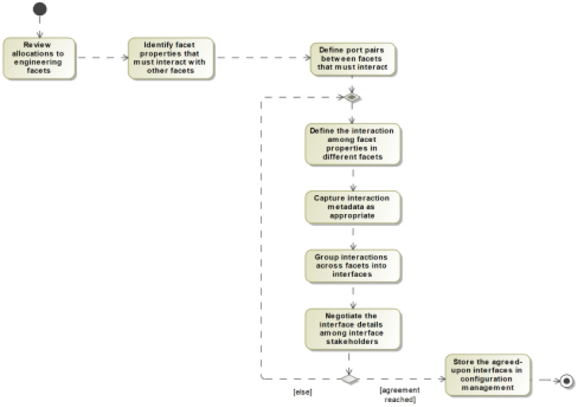
Figure 4.37: Define interdisciplinary interfaces

Review allocations to engineering facets

The previous recipe allocated requirements, values, and functions to the different engineering disciplines. Having a clear understanding of the contributions that must be provided by the engineering facets is a crucial step to creating good interdisciplinary interfaces.

Identify facet properties that must interact with other facets

Interfaces are all about defining the interactions between collaborating elements. In this case, we want to focus on the coordination of elements in different engineering facets. The previous recipe decomposed subsystem features into features within different engineering disciplines. The task here is to relate the properties in collaborating facets.

For example, an electronic sensor may provide a value to the software for manipulation and use, so the device driver (in the software facet) must interact with the actual sensor (in the electronics facet). This interaction will result in a service or flow connection of some kind.

Define port pairs between facets that must interact

Once we have identified that properties in two facets must interact, we define a port pair between the facets to convey the values or service invocations that will be added to the interface.

Define the interaction among facet properties in different facets

The exact nature of the interaction between the facets must be captured in the interface. For example, the software sensor device driver may write to a hardware register to signal the sensor to read a value, wait at least 1 ms, read the sensed value from another hardware register, and then scale the value to what the software needs to manipulate. This interaction and use must be clear in the interface specification.

Capture interaction metadata as appropriate

Metadata is “data about data.” In this case, we use metadata to capture the aspects of an interface that may not be obvious or easy to model in other ways. For example, the previous paragraph provided a simple example of the interaction of a software device driver with an electronic sensor. Relevant metadata would be the memory map address of the hardware registers and the bit-mapping of the values in the registers. For example, in the sensor control register, writing a 1 to bit 0 might activate the sensor, while writing a 0 bit to the same register has no effect; the value from bits 1–5 might provide a read-only error code should the electronics fail. The fact that the software must wait for 1 ms after activating the sensor before reading the value must be captured in the interface as metadata if the software and electronics are to work together properly.

Group interactions across facets into interfaces

All the interactions between the facets must be captured in interfaces. These interfaces must contain relevant information about the interfaces, including how they are accessed by the respective facets. This is most obvious with respect to electronic-software interfaces. The two most common technical means for interfacing between software and electronics are memory-mapped registers and hardware-generated software interrupts.

Negotiate the interface details among interface stakeholders

Keep in mind in this step is that the engineering disciplines must be free to develop their facets using their hard-won engineering skills without being overly encumbered by expectations from other engineering disciplines.

In other words, the systems or software engineers shouldn’t dictate the electronics design and the systems or electronics engineers shouldn’t dictate the design of the software. Nevertheless, the interfaces do specify the overlap between the disciplines. All the stakeholders should agree on the specifications of the interfaces. This includes the systems engineers – who have a stake in overall system optimization – and the involved engineering disciplines.

Store the agreed-upon interfaces in configuration management

There should always be a “known target” for the interfaces between facets even if that interface changes in the future. Yes, changing interfaces downstream will entail some amount of rework, but in practice, it is much less rework than if agreements aren’t there in the first place. The worst outcomes occur when the disciplines continue without a shared understanding of those interfaces. Storing the interfaces under configuration management establishes a baseline and a source of truth from which the engineering disciplines can draw. Should future work uncover some inadequacy of the interfaces, the interfaces can be renegotiated and the configuration-managed baseline updated.

Example

This example will continue from the last recipe with the definition of the Power Train subsystem interfaces. The example in the previous section detailed the allocated requirements and subsystem features to the disciplines of mechanical, electronic, and software.

Review allocations to engineering facets

Read the example from the previous section to review the requirements, value, and function allocation.

Identify facet properties that must interact with other facets

In an effort to avoid over-specification of the facet designs, let’s limit our concerns to the subsystem features that decomposed into elements mapped into different facets. In the previous example, we added dependencies from the decomposed facet-specific feature to the subsystem block features. Figure 4.38 shows the mapping of facet features to subsystem block features:

Figure 4.38: Subsystem features decomposed to facets

Define port pairs between facets that must interact

We previously defined the port and added empty interfaces to define them. See Figure 4.28.

Define the interaction among facet properties in different facets

This is the interesting part of the recipe: defining exactly how the facets will interact. Because we are using SysML proxy ports, we will capture these as interface blocks as shown in Figure 4.39:

Figure 4.39: Deployment interfaces

The software-electronic interfaces are mostly composed of hardware registers, represented as flow properties. Both the iSW_EE_Control and iSW_EE_Comm interface blocks have control and data registers. The software triggers hardware actions or reads status information with these control registers. The data registers provide raw data from the software to the hardware or from the hardware to the software. The iSW_EE_Comm interface block also has two 64-byte blocks, one for sending a CAN bus message and the other for receiving one. The event receptions indicate interrupts generated by the hardware under different conditions. Also, the electronics-mechanical interface block iEE_ME_Resistance contains a drive train connection value property defined by the special value type chain_drive.

Let’s now consider how the software-electronic interfaces will work, starting with the iSW_EE_Control interface block. In actual practice, this would be an outcome of a discussion between software, electronic, and systems engineers.

The control register in this case will have control or error indication responsibility, each of which requires a single bit:

• Bit 0 will be a software write-only bit that informs the hardware to start monitoring the pedal and providing resistance. When a 1 is written to this bit, the hardware will start applying the force as specified in the resistance hardware register and also start measuring pedal position, pedal speed, and power. The electronics will write those values to the corresponding hardware registers. When a 0 is written to this bit, the electronics stop providing resistance to the pedals and stop measuring pedal and power data. The hardware must assure the software that the updates to any register are all completed within a single CPU cycle to prevent race conditions.
• Bit 1 of the control register is read-only by the software and is used to indicate an error condition in the delivery of power via the motor: a 0 value indicates no error while a 1 indicates an error has occurred.
• Bit 2 of the control register is read-only by the software and indicates an error in the pedal position or pedal speed measurement (0 is no error, 1 indicates an error).
• Bit 3 is an indicator of an error reading power delivered by the rider (0 is no error, 1 indicates an error).
• Bits 4–7 are unused.

The other registers indicate either measured values from the electronics (read-only by the software) or commanded resistance from the software (write-only by the software). The electronics will have their own scale of these values, using either 8 bits (such as for the pedal speed and position) or 16 bits (for resistance and power). The direction of the flow properties is from the software perspective (following our previous convention that the first field in the interface block name indicates the unconjugated side of the interface). However, the range of values represented is not scaled by how the user would interpret the values, but rather by the hardware capability. The software is expected to scale the values to units meaningful elsewhere.

The electronics measures pedal position as an 8-bit value from 0 (right crank vertical) to 255 (almost vertical). Pedal speed is an 8-bit value ranging from 0 (no movement) to 255 (maximum measured speed of the hardware). Resistance is written to the register by the software as a 16-bit value from 0 (no resistance) up to 65,535 (maximum resistance). Likewise, power is a hardware-measured value from 0 (no power) to 65,535 (maximal measured power). The exact scaling factors will be specified by the hardware at a later date.

The iSW_EE_Comm interface is a bit more interesting. The core flow properties are the CAN Receive Buffer and CAN Send Buffer. Each of these is a 64-byte wide, byte-addressable memory register that holds CAN bus messages. The expected interaction flow looks like this:

To send a message:

1. The software checks bit 0 of the CAN control register. If it’s a 0, then data may be written to the CAN Send Buffer. If not, the software must wait.
2. The software then writes the CAN bus message it wants to send into the CAN Send Buffer.
3. The software then writes a 1 to bit 0 of the CAN control register.
4. The hardware sets the read value of this bit to 1.
5. The hardware bangs the bits out on the CAN bus.
6. When the hardware has sent the message, the hardware sets the software read value of bit 0 of the control register to 0.
7. The hardware generates an interrupt 2 to the software to indicate that the CAN Send Buffer is now available.
8. The software may install an interrupt service routine to interrupt 2 (swCANMsgSend) to send the next message if desired.

To receive a message:

1. The hardware begins receiving the CAN bus message, filling in the 64-byte wide CAN Receive Buffer.
2. When the message has been received and stored, the hardware generates interrupt 3 (swCANMsgReceived) and sets the read value of bit 1 of the control register to 1 to indicate that a message is available.
3. The software is expected to either poll bit 1 of the control register or install an interrupt service routine to read the message.
4. Once the software has read the message, it is expected to write a 0 value to bit 1. The hardware ignores this value, but it serves as a flag to the software.

Capture interaction metadata as appropriate

The proper way to interpret the bits of the flow properties and the ordering and timing of actions to properly interact over the interface constitute the metadata of interest. To this end, I created a set of stereotypes for this purpose and put them into a shared common profile (Table 4.3).

Most of these stereotypes have tags to represent metadata of interest about the element, but some stereotypes are simply used to identify a “special kind of thing.” There is some redundancy in the stereotype tags to allow a degree of flexibility in modeling the necessary information:

Stereotype	Applicable to	Tag	Description
bitmapped	Argument Attribute/Value Property Call Operation Class/Block Signal Flow/Flow Property/Item Flow Part Instance Operation Reception	bit_0	Interpretation and use, including read, write, or read/write
		bit_1	Interpretation and use, including read, write, or read/write
		bit_2	Interpretation and use, including read, write, or read/write
		bit_3	Interpretation and use, including read, write, or read/write
		bit_4	Interpretation and use, including read, write, or read/write
		bit_5	Interpretation and use, including read, write, or read/write
		bit_6	Interpretation and use, including read, write, or read/write
		bit_7	Interpretation and use, including read, write, or read/write
		bit_8	Interpretation and use, including read, write, or read/write
		bit_9	Interpretation and use, including read, write, or read/write
		bit_10	Interpretation and use, including read, write, or read/write
		bit_11	Interpretation and use, including read, write, or read/write
		bit_12	Interpretation and use, including read, write, or read/write
		bit_13	Interpretation and use, including read, write, or read/write
		bit_14	Interpretation and use, including read, write, or read/write
		bit_15	Interpretation and use, including read, write, or read/write
		Number_Of_Bits	Which bits are valid
		Start_Address	Memory map starting address
		Timing_Constraints	Timing and delays in use
		Usage	Description of the use of the register overall
bytemapped	Argument Attribute/Value Property Call Operation Class/Block Signal Flow/Flow Property/Item Flow Part Instance Operation Reception	Endianism	Big or little endian
		Format	How to interpret the collection bytes
		Number_Of_Bytes	How many bytes are included in the value
		Start_Address	Memory map starting address
		Starting_Byte_Number	Index into a larger array, if necessary
		Timing_Constraints	Timing and delays in use
		Units	If appropriate, units represented by the value
		Usage	Description of the use of the register overall
interruptmapped	Call Operation Signal Operation Reception	Byte_Width	Byte width of arguments (if any)
		Data_Address	Location of arguments (if any)
		Data_Field_Type	Format/interpretation of arguments (if any)
		Interrupt_number	Interrupt vector #
		Usage	What the interrupt indicates
memorymapped	Argument Attribute/Value Property Call Operation Class/Block Signal Flow/Flow Property/Item Flow Part Instance Operation Reception Triggered Operation	Bitmap	Internal format of the memory-mapped item
		Numer_Of_Bytes	Size (in bytes) of the memory-mapped item
		Range_High	High end of range (if continuous)
		Range_low	Low end of range (if continuous)
		Start_Address	Location of the first element in the memory map
		Timing_Constraints	Timeliness constraints on use
		Usage	Description of the use of the element
<none>digitalVoltage	Attribute/Value Property Class/Block Reception Operation Signal Part Instance	Usage	How to interpret different voltage levels
ee_hy_interface	Attribute/Value property Argument Call Operation Class/Block Part Instance Operation Reception Triggered Operation	<none>	Indicates this interface is between electronics and hydraulics
ee_me_interface	Attribute/Value property Argument Call Operation Class/Block Part Instance Operation Reception Triggered Operation	<none>	Indicates this interface is between electronics and mechanical parts
electrohydraulic	Attribute/Value Property Class/Block Part Instance Operation Reception		Indicates this element is composed of integrated electronics and hydraulics
electronics	Attribute/Value Property Class/Block Part Instance Operation Reception	<none>	Indicates this element is implemented in electronics
hydraulic	Attribute/Value Property Class/Block Part Instance Operation Reception	<none>	Indicates this element is implemented in hydraulics
mechanics	Attribute/Value Property Class/Block Part Instance Operation Reception	<none>	Indicates this element is implemented in mechanics
physicalRealization	Dependency	<none>	Relates a logical element (target) to its physical realization (source)
software	Attribute/Value Property Class/Block Part Instance Operation Reception	<none>	Indicates this element is implemented in software
staticMechanical	Association Link/Connector	<none>	Indicates this relation indicates a mechanical linkage that does not convey a flow (e.g. a static connection, such as bolting something together)
sw_ee_interface	Attribute/Value property Argument Call Operation Class/Block Part Instance Operation Reception Triggered Operation	<none>
voltagemapped	Attribute/Value Property Flow/Flow Property/Item Flow	<none>	Indicates this element represents values via voltage levels

Table 4.3: Some useful handoff stereotypes

We will use these stereotypes to model relevant metadata for the interfaces in our model. The flow properties and event receptions in the interface blocks in Figure 4.39 are elaborated and filled out in Table 4.4:

Interface	Feature	Feature Type	Tag	Value
iEE_ME_Resistance	drive_train_connection	FlowProperty	direction	Bidirectional
iSW_EE_Comm	CAN_control_register	FlowProperty	bit_0	SW read: 0 = data may be written to send buffer; 1 = buffer is in use SW write: 0 = no effect, 1 = signal for electronics to send message
iSW_EE_Comm	CAN_control_register	FlowProperty	bit_1	SW read 0 = no new message, 1 = new message in CAN Receive Buffer SW Write: 0 = value saved to display on next read (otherwise ignored by electronics)
iSW_EE_Comm	CAN_control_register	FlowProperty	direction	Bidirectional
iSW_EE_Comm	CAN_control_register	FlowProperty	Start_Address	A000: A0020
iSW_EE_Comm	CAN_control_register	FlowProperty	Usage	Controls/indicates the status of the CAN message flow
iSW_EE_Comm	CANReceiveBuffer	FlowProperty	direction	In
iSW_EE_Comm	CANReceiveBuffer	FlowProperty	Format	Defined by the CAN Bus Standard
iSW_EE_Comm	CANReceiveBuffer	FlowProperty	Start_Address	A000: 0100
iSW_EE_Comm	CANReceiveBuffer	FlowProperty	Starting_Byte_Number	0
iSW_EE_Comm	CANReceiveBuffer	FlowProperty	Usage	Electronics write the values to the buffer and notify the SW when the complete message is stored.
iSW_EE_Comm	CANSendBuffer	FlowProperty	direction	Out
iSW_EE_Comm	CANSendBuffer	FlowProperty	Format	Defined by the CAN Bus standard
iSW_EE_Comm	CANSendBuffer	FlowProperty	Start_Address	A000: 1200
iSW_EE_Comm	CANSendBuffer	FlowProperty	Usage	SW writes the CAN message to be sent and then notifies the electronics to send the message via the CAN Control Register. Electronics notify the software when the message is sent.
iSW_EE_Comm	swCANMsgReceived	Reception	Interrupt_number	3
iSW_EE_Comm	swCANMsgReceived	Reception	Usage	Electronics generate this interrupt to indicate that a message has been received and is available in the CAN Receive Buffer.
iSW_EE_Comm	swCANMsgSent	Reception	Interrupt_number	2
iSW_EE_Comm	swCANMsgSent	Reception	Usage	Electronics generate interrupt #2 to indicate that the commanded CAN message has been sent.
iSW_EE_Control	control_register	FlowProperty	bit_0	SW WO (Write Only). 0 = do not provide resistance, 1 = provide resistance
iSW_EE_Control	control_register	FlowProperty	bit_1	SW RO (Read Only). 0 = no error in resistance, 1 = error
iSW_EE_Control	control_register	FlowProperty	bit_2	SW RO (Read Only). 0 = no pedal position error, 1 = pedal position error
iSW_EE_Control	control_register	FlowProperty	bit_3	SW RO (Read Only). 0 = no rider power measurement error, 1 = rider power measurement error
iSW_EE_Control	control_register	FlowProperty	direction	Bidirectional
iSW_EE_Control	control_register	FlowProperty	Number_Of_Bits	4
iSW_EE_Control	control_register	FlowProperty	Start_Address	0 x A000 0001
iSW_EE_Control	control_register	FlowProperty	Timing_Constraints	none
iSW_EE_Control	control_register	FlowProperty	Usage	Bit 0 enables/disables power measurement and delivery. Other bits provide error indicators.
iSW_EE_Control	pedal_position	FlowProperty	direction	In
iSW_EE_Control	pedal_position	FlowProperty	Numer_Of_Bytes	1
iSW_EE_Control	pedal_position	FlowProperty	Start_Address	A000: 0002
iSW_EE_Control	pedal_position	FlowProperty	Starting_Byte_Number	0
iSW_EE_Control	pedal_position	FlowProperty	Units	Each value corresponds to 1/256 of a circle.
iSW_EE_Control	pedal_position	FlowProperty	Usage	SW RO (Read Only). Read the value to get the pedal position.
iSW_EE_Control	pedal_speed	FlowProperty	direction	In
iSW_EE_Control	pedal_speed	FlowProperty	Numer_Of_Bytes	1
iSW_EE_Control	pedal_speed	FlowProperty	Start_Address	A000 0004
iSW_EE_Control	pedal_speed	FlowProperty	Units	Each value corresponds to 1/1,608 radians/min (maximum of 256 revs/min).
iSW_EE_Control	pedal_speed	FlowProperty	Usage	SW RO (Read Only). Read this value to get the current velocity of the pedals.
iSW_EE_Control	power	FlowProperty	direction	In
iSW_EE_Control	power	FlowProperty	Units	0 = no resistance, 0 x FFFF = max power (0.046W per step)
iSW_EE_Control	power	FlowProperty	Usage	SW RO (Read Only). Read the value of the power applied to the pedal by the rider.
iSW_EE_Control	resistance	FlowProperty	direction	Out
iSW_EE_Control	resistance	FlowProperty	Format	16-bit value
iSW_EE_Control	resistance	FlowProperty	Numer_Of_Bytes	2
iSW_EE_Control	resistance	FlowProperty	Start_Address	A000: 0006
iSW_EE_Control	resistance	FlowProperty	Starting_Byte_Number	0
iSW_EE_Control	resistance	FlowProperty	Units	0 = no resistance, 0 x FFFF = max resistance (18.3N per step)
iSW_EE_Control	resistance	FlowProperty	Usage	SW Write Only (WO). Specify the resistance to be applied to the rider at the pedal.

Table 4.4: Power train deployment interface metadata

Group interactions across facets into interfaces

We incrementally added the interface block features directly into the interface blocks already, so this step is already done!

Negotiate the interface details among interface stakeholders

Now that we have defined the interface blocks and their features (flow properties and event receptions) and characterized them with metadata, the stakeholders can meet to review and negotiate the interface details. The stakeholders, in this case, include representatives from systems, software, electronics, and mechanical engineering. The interface will define a kind of contract that all parties agree to honor.

Store the agreed-upon interfaces in configuration management

The defined interfaces can now be baselined in configuration management. All parties agree to uphold those interfaces. Should downstream work demonstrate inadequacies or identify problems with the interface, the relevant stakeholders can meet again, renegotiate the interface definition, and get back to engineering.

Join our community on Discord

Join our community’s Discord space for discussions with the author and other readers:

https://packt.link/cpVUC