
Chapter Eleven. Special-Purpose Sorting Methods
Sorting methods are critical components of many applications systems, and it is not unusual for special measures to be taken to make a sort as fast as possible or capable of handling huge files. We might encounter high-performance enhancements to a computer system, or special-purpose hardware specifically designed for sorting, or simply a new computer system based on some new architectural design. In such cases, the implicit assumptions that we have been making about the relative costs of operations on the data to be sorted may not be valid. In this chapter, we examine examples of sorting methods that are designed to run efficiently on various different kinds of machines. We consider several different examples of the restrictions imposed by high-performance hardware, and several methods that are useful in practice for implementing high-performance sorts.
Any new computer architecture is eventually going to need to support an efficient sorting method. Indeed, sorting has historically served as one testbed for evaluating new architectures, because it is so important and so well understood. We want to learn not just which known algorithms run best on a new machine and why, but also whether specific characteristics of a new machine can be exploited in some new algorithm. To develop a new algorithm, we define an abstract machine that encapsulates the essential properties of the real machine; design and analyze algorithms for the abstract machine; then implement, test, and refine both the best algorithms and the model. We draw on our past experience, including the many methods for general-purpose machines that we have seen in Chapters 6 through 10, but the abstract machines impose limitations that help us to focus on the true costs, and make it clear that different algorithms are appropriate for different machines.
At one end of the spectrum, we shall consider low-level models where the only allowed operation is the compare–exchange operation. At the other end of the spectrum, we shall consider high-level models where we read and write large blocks of data to a slow external medium or among independent parallel processors.
First, we examine a version of mergesort known as Batcher’s odd–even mergesort. It is based on a divide-and-conquer merge algorithm that uses only compare–exchange operations, with perfect-shuffle and perfect-unshuffle operations for data movement. These are of interest in their own right, and apply to many problems other than sorting. Next, we examine Batcher’s method as a sorting network. A sorting network is a simple abstraction for low-level sorting hardware. Networks consist of interconnected comparators, which are modules capable of performing compare–exchange operations.
Another important abstract sorting problem is the external-sorting problem, where the file to be sorted is far too large to fit in memory. The cost of accessing individual records can be prohibitive, so we shall use an abstract model, where records are transferred to and from external devices in large blocks. We consider two algorithms for external sorting, and use the model to compare them.
Finally, we consider parallel sorting, for the case when the file to be sorted is distributed among independent parallel processors. We define a simple parallel-machine model, then examine how Batcher’s method provides an effective solution. Our use of the same basic algorithm to solve a high-level problem and a low-level problem is a convincing example of the power of abstraction.
The different abstract machines in this chapter are simple, but are worthy of study because they encapsulate specific constraints that can be critical in particular sorting applications. Low-level sorting hardware has to consist of simple components; external sorts generally require access of huge data files in blocks, with sequential access more efficient than random access; and parallel sorting involves communications constraints among processors. On the one hand, we cannot do justice to detailed machine models that fully correspond to particular real machines; on the other hand, the abstractions that we do consider lead us not only to theoretical formulations that provide information about essential limitations on performance, but also to interesting algorithms that are of direct practical utility.
11.1 Batcher’s Odd–Even Mergesort
To begin, we shall consider a sorting method that is based on just two abstract operations, the compare–exchange operation and the perfect shuffle operation (along with its inverse, the perfect unshuffle). The algorithm, developed by Batcher in 1968, is known as Batcher’s odd–even mergesort. It is a simple task to implement the algorithm using shuffles, compare–exchanges, and double recursion, but it is more challenging to understand why the algorithm works, and to untangle the shuffles and recursion to see how it operates at a low level.
We encountered the compare–exchange operation briefly in Chapter 6, where we noted that some of the elementary sort methods discussed there could be expressed more concisely in terms of this abstract operation. Now, we are interested in methods that examine the data exclusively with compare–exchange operations. Standard comparisons are ruled out: The compare–exchange operation does not return a result, so there is no way for a program to take action that depends on data values.
Definition 11.1 A nonadaptive sorting algorithm is one where the sequence of operations performed depends on only the number of the inputs, rather than on the values of the keys.
In this section, we do allow operations that unilaterally rearrange the data, such as exchanges and perfect shuffles, but they are not essential, as we shall see in Section 11.2. Nonadaptive methods are equivalent to straight-line programs for sorting: They can be expressed simply as a list of the compare–exchange operations to be performed. For example, the sequence
compexch(a[0], a[1])
compexch(a[1], a[2])
compexch(a[0], a[1])
is a straight-line program for sorting three elements. We use loops, shuffles, and other high-level operations for convenience and economy in expressing algorithms, but our goal in developing an algorithm is to define, for each N, a fixed sequence of compexch operations that can sort any set of N keys. We can assume without loss of generality that the key values are the integers 1 through N (see Exercise 11.4); to know that a straight-line program is correct, we have to prove that it sorts each possible permutation of these values (see, for example, Exercise 11.5).
Few of the sorting algorithms that we considered in Chapters 6 through 10 are nonadaptive—they all use less or examine the keys in other ways, then take differing actions depending on key values. One exception is bubble sort (see Section 6.4), which uses only compare–exchanges. Pratt’s version of shellsort (see Section 6.6) is another nonadaptive method.
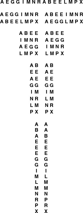
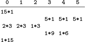
Program 11.1 gives an implementation of the other abstract operations that we shall be using—the perfect shuffle and the perfect unshuffle—and Figure 11.1 gives an example of each. The perfect shuffle rearranges an array in a manner corresponding to the way that a deck of cards might be rearranged when shuffled by an expert: It is split precisely in half, then the cards are taken alternately from each half to make the shuffled deck. We always take the first card from the top half of the deck. If the number of cards is even, the two halves have the same number of cards; if the number of cards is odd, the extra card ends up in the top half. The perfect unshuffle does the opposite: We make the unshuffled deck by putting cards alternately in the top half and the bottom half.
To perform a perfect shuffle (left), we take the first element in the file, then the first element in the second half, then the second element in the file, then the second element in the second half, and so forth. Consider the elements to be numbered starting at 0, top to bottom. Then, elements in the first half go to even-numbered positions, and elements in the second half go to odd-numbered positions. To perform a perfect unshuffle (right), we do the opposite: Elements in even-numbered positions go to the first half, and elements in odd-numbered positions go to the second half.
Figure 11.1 Perfect shuffle and perfect unshuffle
Batcher’s sort is exactly the top-down mergesort of Section 8.3; the difference is that instead of one of the adaptive merge implementations from Chapter 8, it uses Batcher’s odd-even merge, a nonadaptive top-down recursive merge. Program 8.3 does not access the data at all, so our use of a nonadaptive merge implies that the whole sort is nonadaptive.
We shall implicitly assume in the text throughout this section and Section 11.2 that the number of items to be sorted is a power of 2. Then, we can always refer to “N/2” without a caveat about N being odd, and so forth. This assumption is impractical, of course—our programs and examples involve other file sizes—but it simplifies the discussion considerably. We shall return to this issue at the end of Section 11.2.
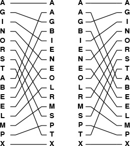
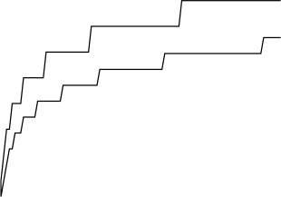
Batcher’s merge is itself a divide-and-conquer recursive method. To do a 1-by-1 merge, we use a single compare–exchange operation. Otherwise, to do an N-by-N merge, we unshuffle to get two N/2-by-N/2 merging problems, and then solve them recursively to get two sorted files. Shuffling these files, we get a file that is nearly sorted—all that is needed is a single pass of N/2 − 1 independent compare–exchange operations: between elements 2i and 2i + 1 for i from 1 to N/2−1. An example is depicted in Figure 11.2. From this description, the implementation in Program 11.2 is immediate.
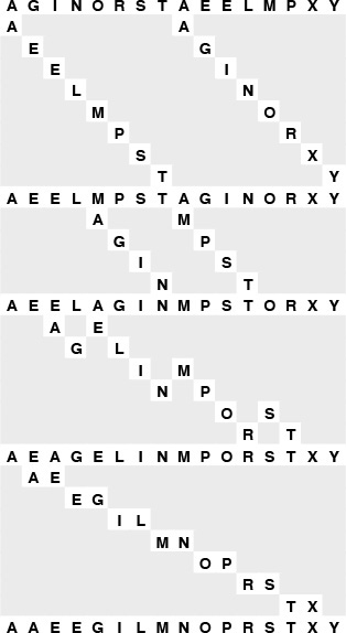
To merge A G I N O R S T with A E E L M P X Y, we begin with an unshuffle operation, which creates two independent merging problems of about one-half the size (shown in the second line): we have to merge A I O S with A E M X (in the first half of the array) and G N R T with E L P Y (in the second half of the array). After solving these subproblems recursively, we shuffle the solutions to these problems (shown in the next-to-last line) and complete the sort by compare–exchanging E with A, G with E, L with I, N with M, P with O, R with S, and T with X.
Figure 11.2 Top-down Batcher’s odd-even merge example
Why does this method sort all possible input permutations? The answer to this question is not at all obvious—the classical proof is an indirect one that depends on a general characteristic of nonadaptive sorting programs.
Property 11.1 (0–1 principle) If a nonadaptive program produces sorted output when the inputs are all either 0 or 1, then it does so when the inputs are arbitrary keys.
See Exercise 11.7. ![]()
Property 11.2 Batcher’s odd–even merge (Program 11.2) is a valid merging method.
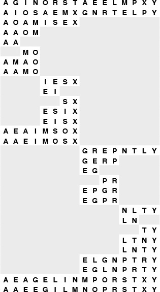
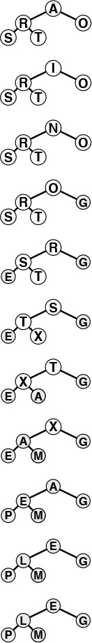
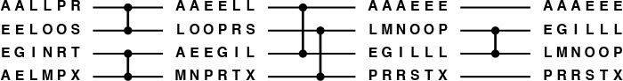
Using the 0–1 principle, we check only that the method properly merges when the inputs are all either 0 or 1. Suppose that there are i 0s in the first subfile and j 0s in the second subfile. The proof of this property involves checking four cases, depending on whether i and j are odd or even. If they are both even, then the two merging subproblems each involve one file with i/2 0s and one file with j/2 0s, so both results have (i + j)/2 0s. Shuffling, we get a sorted 0–1 file. The 0–1 file is also sorted after shuffling in the case that i is even and j is odd and the case that i is odd and j is even. But if both i and j are odd, then we end up shuffling a file with (i + j)/2 + 1 0s with a file with (i + j)/2 − 1 0s, so the 0–1 file after shuffling has i + j − 1 0s, a 1, a 0, then N − i − j − 1 1s (see Figure 11.3), and one of the comparators in the final stage completes the sort. ![]()
These four examples consist of five lines each: a 0-1 merging problem; the result of an unshuffle operation, which gives two merging problems; the result of recursively completing the merges; the result of a shuffle; and the result of the final odd–even compares. The last stage performs an exchange only when the number of 0s in both input files is odd.
Figure 11.3 Four cases for 0-1 merging
We do not need actually to shuffle the data. Indeed, we can use Programs 11.2 and 8.3 to output a straight-line sorting program for any N, by changing the implementations of compexch and shuffle to maintain indices and to refer to the data indirectly (see Exercise 11.12). Or, we can have the program output the compare–exchange instructions to use on the original input (see Exercise 11.13). We could apply these techniques to any nonadaptive sorting method that rearranges the data with exchanges, shuffles, or similar operations. For Batcher’s merge, the structure of the algorithm is so simple that we can develop a bottom-up implementation directly, as we shall see in Section 11.2.
11.2 Generalize Program 11.1 to implement h-way shuffle and unshuffle. Defend your strategy for the case that the file size is not a multiple of h.
![]() 11.3 Implement the shuffle and unshuffle operations without using an auxiliary array.
11.3 Implement the shuffle and unshuffle operations without using an auxiliary array.
![]() 11.4 Show that a straight-line program that sorts N distinct keys will sort N keys that are not necessarily distinct.
11.4 Show that a straight-line program that sorts N distinct keys will sort N keys that are not necessarily distinct.
![]() 11.5 Show how the straight-line program given in the text sorts each of the six permutations of the integers 1, 2, and 3.
11.5 Show how the straight-line program given in the text sorts each of the six permutations of the integers 1, 2, and 3.
![]() 11.6 Give a straight-line program that sorts four elements.
11.6 Give a straight-line program that sorts four elements.
![]() 11.7 Prove Property 11.1. Hint: Show that if the program does not sort some input array with arbitrary keys, then there is some 0–1 sequence that it does not sort.
11.7 Prove Property 11.1. Hint: Show that if the program does not sort some input array with arbitrary keys, then there is some 0–1 sequence that it does not sort.
![]() 11.8 Show how the keys A E Q S U Y E I N O S T are merged using Program 11.2, in the style of the example diagrammed in Figure 11.2.
11.8 Show how the keys A E Q S U Y E I N O S T are merged using Program 11.2, in the style of the example diagrammed in Figure 11.2.
![]() 11.9 Answer Exercise 11.8 for the keys A E S Y E I N O Q S T U.
11.9 Answer Exercise 11.8 for the keys A E S Y E I N O Q S T U.
![]() 11.10 Answer Exercise 11.8 for the keys 1 0 0 1 1 1 0 0 0 0 0 1 0 1 0 0.
11.10 Answer Exercise 11.8 for the keys 1 0 0 1 1 1 0 0 0 0 0 1 0 1 0 0.
11.11 Empirically compare the running time of Batcher’s mergesort with that of standard top-down mergesort (Programs 8.3 and 8.2) for N = 103, 104, 105, and 106.
11.12 Give implementations of compexch, shuffle, and unshuffle that cause Programs 11.2 and 8.3 to operate as an indirect sort (see Section 6.8).
![]() 11.13 Give implementations of
11.13 Give implementations of compexch, shuffle, and unshuffle that cause Programs 11.2 and 8.3 to print out, given N, a straight-line program for sorting N elements. You may use an auxiliary global array to keep track of indices.
11.14 If we put the second file for the merge in reverse order, we have a bitonic sequence, as defined in Section 8.2. Changing the final loop in Program 11.2 to start at l instead of l+1 turns the program into one that sorts bitonic sequences. Show how the keys A E S Q U Y T S O N I E are merged using this method, in the style of the example diagrammed in Figure 11.2.
![]() 11.15 Prove that the modified Program 11.2 described in Exercise 11.14 sorts any bitonic sequence.
11.15 Prove that the modified Program 11.2 described in Exercise 11.14 sorts any bitonic sequence.
11.2 Sorting Networks
The simplest model for studying nonadaptive sorting algorithms is an abstract machine that can access the data only through compare–exchange operations. Such a machine is called a sorting network. A sorting network comprises atomic compare–exchange modules, or comparators, which are wired together so as to implement the capability to perform fully general sorting.
Figure 11.4 shows a simple sorting network for four keys. Customarily, we draw a sorting network for N items as a sequence of N horizontal lines, with comparators connecting pairs of lines. We imagine that the keys to be sorted pass from right to left through the network, with a pair of numbers exchanged if necessary to put the smaller on top whenever a comparator is encountered.
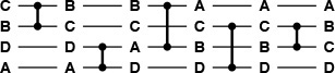
The keys move from left to right on the lines in the network. The comparators that they encounter exchange the keys if necessary to put the smaller one on the higher line. In this example, B and C are exchanged on the top two lines, then A and D are exchanged on the bottom two, then A and B, and so forth, leaving the keys in sorted order from top to bottom at the end. In this example, all the comparators do exchanges except the fourth one. This network sorts any permutation of four keys.
Figure 11.4 A sorting network
Many details must be worked out before an actual sorting machine based on this scheme could be built. For example, the method of encoding the inputs is left unspecified. One approach would be to think of each wire in Figure 11.4 as a group of lines, each holding 1 bit of data, so that all the bits of a key flow through a line simultaneously. Another approach would be to have the comparators read their inputs 1 bit at a time along a single line (most significant bit first). Also left unspecified is the timing: mechanisms must be included to ensure that no comparator performs its operation before its input is ready. Sorting networks are a good abstraction because they allow us to separate such implementation considerations from higher-level design considerations, such as minimizing the number of comparators. Moreover, as we shall see in Section 11.5, the sort network abstraction is useful for applications other than direct circuit realizations.
Another important application of sorting networks is as a model for parallel computation. If two comparators do not use the same input lines, we assume that they can operate at the same time. For example, the network in Figure 11.4 shows that four elements can be sorted in three parallel steps. The 0–1 comparator and the 2–3 comparator can operate simultaneously in the first step, then the 0–2 comparator and the 1–3 comparator can operate simultaneously in the second step, and then the 2–3 comparator finishes the sort in the third step. Given any network, it is not difficult to classify the comparators into a sequence of parallel stages that consist of groups of comparators that can operate simultaneously (see Exercise 11.17). For efficient parallel computation, our challenge is to design networks with as few parallel stages as possible.
Program 11.2 corresponds directly to a merging network for each N, but it is also instructive for us to consider a direct bottom-up construction, which is illustrated in Figure 11.5. To construct a merging network of size N, we use two copies of the network of size N/2; one for the even-numbered lines and one for the odd-numbered lines. Because the two sets of comparators do not interfere, we can rearrange them to interleave the two networks. Then, at the end, we complete the network with comparators between lines 1 and 2, 3 and 4, and so forth. The odd–even interleaving replaces the perfect shuffle in Program 11.2. The proof that these networks merge properly is the same as that given for Properties 11.1 and 11.2, using the 0–1 principle. Figure 11.6 shows an example of the merge in operation.
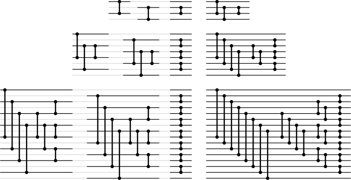
These different representations of the networks for four (top), eight (center), and 16 (bottom) lines expose the network’s basic recursive structure. On the left are direct representations of the construction of the networks of size N with two copies of the networks of size N/2 (one for the even-numbered lines and one for the odd-numbered lines), plus a stage of comparators between lines 1 and 2, 3 and 4, 5 and 6, and so forth. On the right are simpler networks that we derive from those on the left by grouping comparators of the same length; grouping is possible because we can move comparators on odd lines past those on even lines without interference.
Figure 11.5 Batcher’s odd–even merging networks
When all the shuffling is removed, Batcher’s merge for our example amounts to the 25 compare–exchange operations depicted here. They divide into four phases of independent compare–exchange operations at a fixed offset for each phase.
Figure 11.6 Bottom-up Batcher’s merge example
Program 11.3 is a bottom-up implementation of Batcher’s merge, with no shuffling, that corresponds to the networks in Figure 11.5. This program is a compact and elegant in-place merging function that is perhaps best understood as just an alternate representation of the networks, although direct proofs that it accomplishes the merging task correctly are also interesting to contemplate. We shall examine one such proof at the end of this section.
Figure 11.7 shows Batcher’s odd–even sorting network, built from the merging networks in Figure 11.5 using the standard recursive mergesort construction. The construction is doubly recursive: once for the merging networks and once for the sorting networks. Although they are not optimal—we shall discuss optimal networks shortly—these networks are efficient.
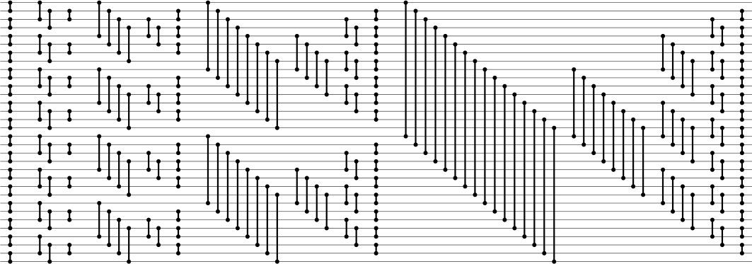
This sorting network for 32 lines contains two copies of the network for 16 lines, four copies of the network for eight lines, and so forth. Reading from right to left, we see the structure in a top-down manner: A sorting network for 32 lines consists of a 16-by-16 merging network following two copies of the sorting network for 16 lines (one for the top half and one for the bottom half). Each network for 16 lines consists of an 8-by-8 merging network following two copies of the sorting network for 8 lines, and so forth. Reading from left to right, we see the structure in a bottom-up manner: The first column of comparators creates sorted subfiles of size 2; then, we have 2-by-2 merging networks that create sorted subfiles of size 4; then, 4-by-4 merging networks that create sorted subfiles of size 8, and so forth.
Figure 11.7 Batcher’s odd–even sorting networks
Property 11.3 Batcher’s odd–even sorting networks have about N(lg N)2/4 comparators and can run in (lg N)2/2 parallel steps.
The merging networks need about lg N parallel steps, and the sorting networks need 1 + 2 + ... + lg N, or about (lg N)2/2 parallel steps. Comparator counting is left as an exercise (see Exercise 11.23). ![]()
Using the merge function in Program 11.3 within the standard recursive mergesort in Program 8.3 gives a compact in-place sorting method that is nonadaptive and uses O(N(lg N)2) compare–exchange operations. Alternatively, we can remove the recursion from the mergesort and implement a bottom-up version of the whole sort directly, as shown in Program 11.4. As was Program 11.3, this program is per haps best understood as an alternate representation of the network in Figure 11.7. The implementation involves adding one loop and adding one test in Program 11.3, because the merge and the sort have similar recursive structure. To perform the bottom-up pass of merging a sequence of sorted files of length 2k into a sequence of sorted files of length 2k + 1, we use the full merging network, but include only those comparators that fall completely within subfiles. This program perhaps wins the prize as the most compact nontrivial sort implementation that we have seen, and it is likely to be the method of choice when we want to take advantage of high-performance architectural features to develop a high-speed sort for small files (or to build a sorting network). Understanding how and why the program sorts would be a formidable task if we did not have the perspective of the recursive implementations and network constructions that we have been considering.
As usual with divide-and-conquer methods, we have two basic choices when N is not a power of 2 (see Exercises 11.24 and 11.21). We can divide in half (top-down) or divide at the largest power of 2 less than N (bottom-up). The latter is somewhat simpler for sorting networks, because it is equivalent to building a full network for the smallest power of 2 greater than or equal to N, then using only the first N lines and only comparators with both ends connected to those lines. The proof that this construction is valid is simple. Suppose that the lines that are not used have sentinel keys that are greater than any other keys on the network. Then, comparators on those lines never exchange, so removing them has no effect. Indeed, we could use any contiguous set of N lines from the larger network: Consider ignored lines at the top to have small sentinels and ignored lines at the bottom to have large sentinels. All these networks have about N(lg N)2/4 comparators.
The theory of sorting networks has an interesting history (see reference section). The problem of finding networks with as few comparators as possible was posed by Bose before 1960, and is called the Bose–Nelson problem. Batcher’s networks were the first good solution to the problem, and for some time people conjectured that they were optimal. Batcher’s merging networks are optimal, so any sorting network with substantially fewer comparators has to be constructed with an approach other than recursive mergesort. The problem of finding optimal sorting networks eluded researchers until, in 1983, Ajtai, Komlos, and Szemeredi proved the existence of networks with O(N log N) comparators. However, the AKS networks are a mathematical construction that is not at all practical, and Batcher’s networks are still among the best available for practical use.
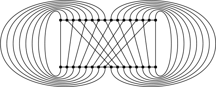
The connection between perfect shuffling and Batcher’s networks makes it amusing to complete our study of sorting networks by considering yet another version of the algorithm. If we shuffle the lines in Batcher’s odd–even merge, we get networks where all the comparators connect adjacent lines. Figure 11.8 illustrates a network that corresponds to the shuffling implementation corresponding to Program 11.2. This interconnection pattern is sometimes called a butterfly network. Also shown in the figure is another representation of the same straight-line program that provides an even more uniform pattern; it involves only full shuffles.
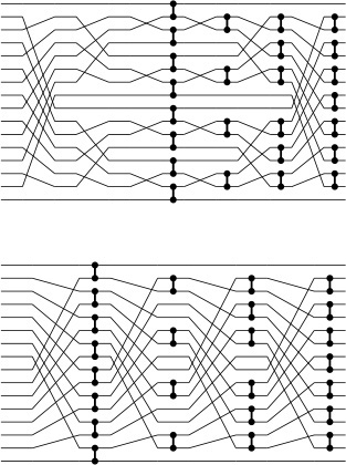
A direct implementation of Program 11.2 as a sorting network gives a network replete with recursive unshuffling and shuffling (top). An equivalent implementation (bottom) involves only full shuffles.
Figure 11.8 Shuffling in Batcher’s odd–even merge
Figure 11.9 shows yet another interpretation of the method that illustrates the underlying structure. First, we write one file below the other; then, we compare those elements that are vertically adjacent and exchange them if necessary to put the larger one below the smaller one. Next, we split each row in half and interleave the halves, then perform the same compare–exchange operations on the numbers in the second and third lines. Comparisons involving other pairs of rows are not necessary because of the previous sorting. The split-interleave operation keeps both the rows and the columns of the table sorted. This property is preserved in general by the same operation: Each step doubles the number of rows, halves the number of columns, and still keeps the rows and the columns sorted; eventually we end up with 1 column of N rows, which is therefore completely sorted. The connection between the tableaux in Figure 11.9 and the network at the bottom in Figure 11.8 is that, when we write down the tables in column-major order (the elements in the first column followed by the elements in the second column, and so forth), we see that the permutation required to go from one step to the next is none other than the perfect shuffle.
Starting with two sorted files in one row, we merge them by iterating the following operation: split each row in half and interleave the halves (left), and do compare-exchanges between items now vertically adjacent that came from different rows (right). At the beginning we have 16 columns and one row, then eight columns and two rows, then four columns and four rows, then two columns and eight rows, and finally 16 rows and one column, which is sorted.
Figure 11.9 Split-interleave merging
Now, with an abstract parallel machine that has the perfect-shuffle interconnection built in, as shown in Figure 11.10, we would be able to implement directly networks like the one at the bottom of Figure 11.8. At each step, the machine does compare–exchange operations between some pairs of adjacent processors, as indicated by the algorithm, then performs a perfect shuffle of the data. Programming the machine amounts to specifying which pairs of processors should do compare–exchange operations at each cycle.
A machine with the interconnections drawn here could perform Batcher’s algorithm (and many others) efficiently. Some parallel computers have connections like these.
Figure 11.10 A perfect shuffling machine
Figure 11.11 shows the dynamic characteristics of both the bottom-up method and this full-shuffling version of Batcher’s odd-even merge.
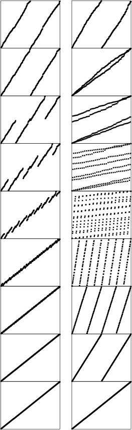
The bottom-up version of the odd–even merge (left) involves a sequence of stages where we compare–exchange the large half of one sorted subfile with the small half of the next. With full shuffling (right), the algorithm has an entirely different appearance.
Figure 11.11 Dynamic characteristics of odd–even merging
Shuffling is an important abstraction for describing data movement in divide-and-conquer algorithms, and it arises in a variety of problems other than sorting. For example, if a 2n-by-2n square matrix is kept in row-major order, then n perfect shuffles will transpose the matrix (convert the matrix to column-major order). More important examples include the fast Fourier transform and polynomial evaluation (see Part 8). We can solve each of these problems using a cycling perfect-shuffle machine like the one shown in Figure 11.10 but with more powerful processors. We might even contemplate having general-purpose processors that can shuffle and unshuffle (some real machines of this type have been built); we return to the discussion of such parallel machines in Section 11.5.
Exercises
11.16 Give sorting networks for four (see Exercise 11.6), five, and six elements. Use as few comparators as possible.
![]() 11.17 Write a program to compute the number of parallel steps required for any given straight-line program. Hint: Use the following labeling strategy. Label the input lines as belonging to stage 0, then do the following for each comparator: Label both output lines as inputs to stage i + 1 if the label on one of the input lines is i and the label on the other is not greater than i.
11.17 Write a program to compute the number of parallel steps required for any given straight-line program. Hint: Use the following labeling strategy. Label the input lines as belonging to stage 0, then do the following for each comparator: Label both output lines as inputs to stage i + 1 if the label on one of the input lines is i and the label on the other is not greater than i.
11.18 Compare the running time of Program 11.4 with that of Program 8.3, for randomly ordered keys with N = 103, 104, 105, and 106.
![]() 11.19 Draw Batcher’s network for doing a 10-by-11 merge.
11.19 Draw Batcher’s network for doing a 10-by-11 merge.
![]() 11.20 Prove the relationship between recursive unshuffling and shuffling that is suggested by Figure 11.8.
11.20 Prove the relationship between recursive unshuffling and shuffling that is suggested by Figure 11.8.
![]() 11.21 From the argument in the text, there are 11 networks for sorting 21 elements hidden in Figure 11.7. Draw the one among these that has the fewest comparators.
11.21 From the argument in the text, there are 11 networks for sorting 21 elements hidden in Figure 11.7. Draw the one among these that has the fewest comparators.
11.22 Give the number of comparators in Batcher’s odd–even sorting networks for 2 ≤ N ≤ 32, where networks when N is not a power of 2 are derived from the first N lines of the network for the next largest power of 2.
![]() 11.23 For N = 2n, derive an exact expression for the number of comparators used in Batcher’s odd–even sorting networks. Note: Check your answer against Figure 11.7, which shows that the networks have 1, 3, 9, 25, and 65 comparators for N equal to 2, 4, 8, 16, and 32, respectively.
11.23 For N = 2n, derive an exact expression for the number of comparators used in Batcher’s odd–even sorting networks. Note: Check your answer against Figure 11.7, which shows that the networks have 1, 3, 9, 25, and 65 comparators for N equal to 2, 4, 8, 16, and 32, respectively.
![]() 11.24 Construct a sorting network for sorting 21 elements using a top-down recursive style, where a network of size N is a composition of networks of sizes
11.24 Construct a sorting network for sorting 21 elements using a top-down recursive style, where a network of size N is a composition of networks of sizes ![]() N/2
N/2![]() and
and ![]() N/2
N/2![]() followed by a merging network. (Use your answer from Exercise 11.19 as the final part of the network.)
followed by a merging network. (Use your answer from Exercise 11.19 as the final part of the network.)
11.25 Use recurrence relations to compute the number of comparators in sorting networks constructed as described in Exercise 11.24 for 2 ≤ N ≤ 32. Compare your results with those that you obtained in Exercise 11.22.
![]() 11.26 Find a 16-line sorting network that uses fewer comparators than Batcher’s network does.
11.26 Find a 16-line sorting network that uses fewer comparators than Batcher’s network does.
11.27 Draw the merging networks corresponding to Figure 11.8 for bitonic sequences, using the scheme described in Exercise 11.14.
11.28 Draw the sorting network corresponding to shellsort with Pratt’s increments (see Section 6.6), for N = 32.
11.29 Give a table containing the number of comparators in the networks described in Exercise 11.28 and the number of comparators in Batcher’s networks, for N = 16, 32, 64, 128, and 256.
11.30 Design sorting networks that will sort files of N elements that are 3-and 4-sorted.
![]() 11.31 Use your networks from Exercise 11.30 to design a Pratt-like scheme based on multiples of 3 and 4. Draw your network for N = 32, and answer Exercise 11.29 for your networks.
11.31 Use your networks from Exercise 11.30 to design a Pratt-like scheme based on multiples of 3 and 4. Draw your network for N = 32, and answer Exercise 11.29 for your networks.
![]() 11.32 Draw a version of Batcher’s odd–even sorting network for N = 16 that has perfect shuffles between stages of independent comparators connecting adjacent lines. (The final four stages of the network should be those from the merging network at the bottom of Figure 11.8.)
11.32 Draw a version of Batcher’s odd–even sorting network for N = 16 that has perfect shuffles between stages of independent comparators connecting adjacent lines. (The final four stages of the network should be those from the merging network at the bottom of Figure 11.8.)
![]() 11.33 Write a merging program for the machine in Figure 11.10, using the following conventions. An instruction is a sequence of 15 bits, where the ith bit, for 1 ≤ i ≤ 15, indicates (if it is 1) that processor i and processor i – 1 should do a compare–exchange. A program is a sequence of instructions, and the machine executes a perfect shuffle between each instruction.
11.33 Write a merging program for the machine in Figure 11.10, using the following conventions. An instruction is a sequence of 15 bits, where the ith bit, for 1 ≤ i ≤ 15, indicates (if it is 1) that processor i and processor i – 1 should do a compare–exchange. A program is a sequence of instructions, and the machine executes a perfect shuffle between each instruction.
![]() 11.34 Write a sorting program for the machine in Figure 11.10, using the conventions described in Exercise 11.33.
11.34 Write a sorting program for the machine in Figure 11.10, using the conventions described in Exercise 11.33.
11.3 External Sorting
We move next to another kind of abstract sorting problem, which applies when the file to be sorted is much too large to fit in the random-access memory of the computer. We use the term external sorting to describe this situation. There are many different types of external sorting devices, which can place a variety of different restrictions on the atomic operations used to implement the sort. Still, it is useful to consider sorting methods that use two basic primitive operations: read data from external storage into main memory, and write data from main memory onto external storage. We assume that the cost of these two operations is so much larger than the cost of primitive computational operations that we ignore the latter entirely. For example, in this abstract model, we ignore the cost of sorting the main memory! For huge memories or poor sorting methods, this assumption may not be justified; but it is generally possible to factor in an estimate of the true cost in practical situations if necessary.
The wide variety of types and costs of external storage devices makes the development of external sorting methods highly dependent on current technology. These methods can be complicated, and many parameters affect their performance; that a clever method might go unappreciated or unused because of a simple change in the technology is certainly a possibility in the study of external sorting. For this reason, we shall concentrate on reviewing general methods rather than on developing specific implementations in this section.
Over and above the high read–write cost for external devices, there are often severe restrictions on access, depending on the device. For example, for most types of devices, read and write operations between main memory and external storage are generally done most efficiently in large contiguous blocks of data. Also, external devices with huge capacities are often designed such that peak performance is achieved when we access the blocks in a sequential manner. For example, we cannot read items at the end of a magnetic tape without first scanning through items at the beginning—for practical purposes, our access to items on the tape is restricted to those appearing somewhere close to the items most recently accessed. Several modern technologies have this same property. Accordingly, in this section, we concentrate on methods that read and write large blocks of data sequentially, making the implicit assumption that fast implementations of this type of data access can be achieved for the machines and devices that are of interest.
When we are in the process of reading or writing a number of different files, we assume that they are all on different external storage devices. On ancient machines, where files were stored on externally mounted magnetic tapes, this assumption was an absolute requirement. When working with disks, it is possible to implement the algorithms that we consider using only a single external device, but it generally will be much more efficient to use multiple devices.
A first step for someone planning to implement an efficient program to sort a huge file might be to implement an efficient program to make a copy of the file. A second step might be to implement a program to reverse the order of the file. Whatever difficulties arise in solving these tasks certainly need to be addressed in implementing an external sort. (The sort might have to do either one of them.) The purpose of using an abstract model is to allow us to separate such implementation issues from algorithm design issues.
The sorting algorithms that we examine are organized as a number of passes over all the data, and we usually measure the cost of an external sorting method by simply counting the number of such passes. Typically, we need relatively few passes—perhaps ten or fewer. This fact implies that eliminating even a single pass can significantly improve performance. Our basic assumption is that the running time of an external sorting method is dominated by input and output; thus, we can estimate the running time of an external sort by multiplying the number of passes it uses by the time required to read and write the whole file.
In summary, the abstract model that we shall use for external sorting involves a basic assumption that the file to be sorted is far too large to fit in main memory, and accounts for two other resources: running time (number of passes through the data) and the number of external devices available for use. We assume that we have
• N records to be sorted, on an external device
• space in the main memory to hold M records and
• 2P external devices for use during the sort.
We assign the the label 0 to the external device containing the input, and the labels 1, 2, ..., 2P − 1 to the others. The goal of the sort is to put the records back onto device 0, in sorted order. As we shall see, there is a tradeoff between P and the total running time—we are interested in quantifying that tradeoff so that we can compare competing strategies.
There are many reasons why this idealized model may not be realistic. Still, like any good abstract model, it does capture the essential aspects of the situation, and it does provide a precise framework within which we can explore algorithmic ideas, many of which are of direct utility in practical situations.
Most external sorting methods use the following general strategy. Make a first pass through the file to be sorted, breaking it up into blocks about the size of the internal memory, and sort these blocks. Then, merge the sorted blocks together, if necessary by making several passes through the file, creating successively larger sorted blocks until the whole file is sorted. This approach is called sort–merge, and it has been used effectively since computers first found widespread use in commercial applications in the 1950s.
The simplest sort–merge strategy, which is called balanced multiway merging, is illustrated in Figure 11.12. The method consists of an initial distribution pass, followed by several multiway merging passes.
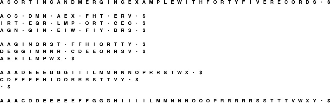
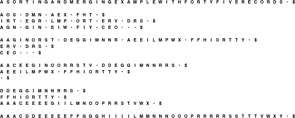
In the initial distribution pass, we take the elements A S O from the input, sort them, and put the sorted run A O S on the first output device. Next, we take the elements R T I from the input, sort them, and put the sorted run I R T on the second output device. Continuing in this way, cycling through the output devices, we end with 15 runs: five on each output device. In the first merging phase, we merge A O S, I R T, and A G N to get A A G I O R S T, which we put on the first output device; then, we merge the second runs on the input devices to get D E G G I M N N R, which we put on the second output device; and so forth; again ending up with the data distributed in a balanced manner on three devices. We complete the sort with two additional merging passes.
Figure 11.12 Three-way balanced merge example
In the initial distribution pass, we distribute the input among external devices P, P + 1, ..., 2P − 1, in sorted blocks of M records each (except possibly the final block, which is smaller, if N is not a multiple of M). This distribution is easy to do—we read the first M records from the input, sort them, and write the sorted block onto device P ; then read the next M records from the input, sort them, and write the sorted block onto device P + 1; and so forth. If, after reaching device 2P − 1 we still have more input (that is, if N > PM), we put a second sorted block on device P, then a second sorted block on device P + 1, and so forth. We continue in this way until the input is exhausted. After the distribution, the number of sorted blocks on each device is N/M rounded up or down to the next integer. If N is a multiple of M, then all the blocks are of size N/M (otherwise, all but the final one are of size N/M). For small N, there may be fewer than P blocks, and one or more of the devices may be empty.
In the first multiway merging pass, we regard devices P through 2P − 1 as input devices, and devices 0 through P − 1 as output devices. We do P-way merging to merge the sorted blocks of size M on the input devices into sorted blocks of size PM, then distribute them onto the output devices in as balanced a manner as possible. First, we merge together the first block from each of the input devices and put the result onto device 0; then, we put the result of merging the second block on each input device onto device 1; and so forth. After reaching device P − 1, we put a second sorted block on device 0, then a second sorted block on device 1, and so forth. We continue in this way until the inputs are exhausted. After the distribution, the number of sorted blocks on each device is N/(PM) rounded up or down to the next integer. If N is a multiple of PM, then all the blocks are of size PM (otherwise, the final block is smaller). If N is not larger than PM, there is just one sorted block left (on device 0), and we are finished.
Otherwise, we iterate the process and do a second multiway merging pass, regarding devices 0, 1, ..., P − 1 as the input devices, and devices P, P + 1, ..., 2P − 1 as the output devices. We do P-way merging to make the sorted blocks of size PM on the input devices into sorted blocks of size P2M, then distribute them back onto the output devices. We are finished after the second pass (with the result on device P) if N is not larger than P2M.
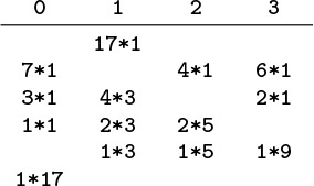
Continuing in this way, back and forth between devices 0 through P − 1 and devices P through 2P − 1, we increase the size of the blocks by a factor of P through P-way merges until we eventually have just one block, on device 0 or on device P. The final merge in each pass may not be a full P-way merge; otherwise the process is well balanced. Figure 11.13 depicts the process using only the numbers and relative sizes of the runs. We measure the cost of the merge by performing the indicated multiplications in this table, summing the results (not including the entry in the bottom row), and dividing by the initial number of runs. This calculation gives cost in terms of the number of passes over the data.
In the initial distribution for a balanced three-way sort–merge of a file 15 times the size of the internal memory, we put five runs of relative size 1 on devices 3, 4, and 5, leaving devices 0, 1, and 2 empty. In the first merging phase, we put two runs of size 3 on devices 0 and 1, and one run of size 3 on device 2, leaving devices 3, 4, and 5 empty. Then, we merge the runs on devices 0, 1, and 2, and distribute them back to devices 3, 4, and 5, and so forth, continuing until only one run remains, on device 0. The total number of records processed is 60: four passes over all 15 records.
Figure 11.13 Run distribution for balanced 3-way merge
To implement P-way merging, we can use a priority queue of size P. We want to output repeatedly the smallest of the elements not yet output from each of the P sorted blocks to be merged, then to replace the element output with the next element from the block from which it came. To accomplish this action, we keep device indices in the priority queue, with a less function that reads the value of the key of the next record to be read from the indicated device (and provides a sentinel larger than all keys in records when the end of a block is reached). The merge is then a simple loop that reads the next record from the device having the smallest key and writes that record to the output, then replaces that record on the priority queue with the next record from the same device, continuing until a sentinel key is the smallest in the priority queue. We could use a heap implementation to make the time required for the priority queue proportional to log P, but P is normally so small that this cost is dwarfed by the cost of writing to external storage. In our abstract model, we ignore priority-queue costs and assume that we have efficient sequential access to data on external devices, so that we can measure running time by counting the number of passes through the data. In practice, we might use an elementary priority-queue implementation and focus our programming on making sure that the external devices run at maximum efficiency.
Property 11.4 With 2P external devices and internal memory sufficient to hold M records, a sort–merge that is based on a P-way balanced merge takes about 1 + ![]() logP (N/M)
logP (N/M)![]() passes.
passes.
One pass is required for distribution. If N = MPk, the blocks are all of size MP after the first merge, MP2 after the second, MP3 after the third; and so forth. The sort is complete after k = logP (N/M) passes. Otherwise, if MPk−1 < N < MPk, the effect of incomplete and empty blocks makes the blocks vary in size near the end of the process, but we are still finished after k = ![]() logP (N/M)
logP (N/M)![]() passes.
passes. ![]()
For example, if we want to sort 1 billion records using six devices and enough internal memory to hold 1 million records, we can do so with a three-way sort–merge with a total of eight passes through the data—one for distribution and ![]() log3 1000
log3 1000![]() = 7 merging passes. We will have sorted runs of 1 million records after the distribution pass, 3 million records after the first merge, 9 million records after the second merge, 27 million records after the third merge, and so forth. We can estimate that it should take about nine times as long to sort the file as it does to copy the file.
= 7 merging passes. We will have sorted runs of 1 million records after the distribution pass, 3 million records after the first merge, 9 million records after the second merge, 27 million records after the third merge, and so forth. We can estimate that it should take about nine times as long to sort the file as it does to copy the file.
The most important decision to be made in a practical sort–merge is the choice of the value of P, the order of the merge. In our abstract model, we are restricted to sequential access, which implies that P has to be one-half the number of external devices available for use. This model is a realistic one for many external storage devices. For many other devices, however, nonsequential access is possible—it is just more expensive than sequential access. If only a few devices are available for the sort, nonsequential access might be unavoidable. In such cases, we can still use multiway merging, but we will have to take into account the basic tradeoff that increasing P will decrease the number of passes but increase the amount of (slow) nonsequential access.
Exercises
![]() 11.35 Show how the keys E A S Y Q U E S T I O N W I T H P L E N T Y O F K E Y S are sorted using 3-way balanced merging, in the style of the example diagrammed in Figure 11.12.
11.35 Show how the keys E A S Y Q U E S T I O N W I T H P L E N T Y O F K E Y S are sorted using 3-way balanced merging, in the style of the example diagrammed in Figure 11.12.
![]() 11.36 What would be the effect on the number of passes used in multiway merging if we were to double the number of external devices in use?
11.36 What would be the effect on the number of passes used in multiway merging if we were to double the number of external devices in use?
![]() 11.37 What would be the effect on the number of passes used in multiway merging if we were to increase by a factor of 10 the amount of internal memory available?
11.37 What would be the effect on the number of passes used in multiway merging if we were to increase by a factor of 10 the amount of internal memory available?
![]() 11.38 Develop an interface for external input and output that involves sequential transfer of blocks of data from external devices that operate asynchronously (or learn details about an existing one on your system). Use the interface to implement P-way merging, with P as large as you can make it while still arranging for the P input files and the input file to be on different output devices. Compare the running time of your program with the time required to copy the files to the output, one after another.
11.38 Develop an interface for external input and output that involves sequential transfer of blocks of data from external devices that operate asynchronously (or learn details about an existing one on your system). Use the interface to implement P-way merging, with P as large as you can make it while still arranging for the P input files and the input file to be on different output devices. Compare the running time of your program with the time required to copy the files to the output, one after another.
![]() 11.39 Use the interface from Exercise 11.38 to write a program to reverse the order of as large a file as is feasible on your system.
11.39 Use the interface from Exercise 11.38 to write a program to reverse the order of as large a file as is feasible on your system.
![]() 11.40 How would you do a perfect shuffle of all the records on an external device?
11.40 How would you do a perfect shuffle of all the records on an external device?
![]() 11.41 Develop a cost model for multiway merging that encompasses algorithms that can switch from one file to another on the same device, at a fixed cost that is much higher than the cost of a sequential read.
11.41 Develop a cost model for multiway merging that encompasses algorithms that can switch from one file to another on the same device, at a fixed cost that is much higher than the cost of a sequential read.
![]() 11.42 Develop an external sorting approach that is based on partitioning a la quicksort or MSD radix sort, analyze it, and compare it with multiway merge. You may use a high level of abstraction, as we did in the description of sort–merge in this section, but you should strive to be able to predict the running time for a given number of devices and a given amount of internal memory.
11.42 Develop an external sorting approach that is based on partitioning a la quicksort or MSD radix sort, analyze it, and compare it with multiway merge. You may use a high level of abstraction, as we did in the description of sort–merge in this section, but you should strive to be able to predict the running time for a given number of devices and a given amount of internal memory.
11.43 How would you sort the contents of an external device if no other devices (except main memory) were available for use?
11.44 How would you sort the contents of an external device if only one extra device (and main memory) was available for use?
11.4 Sort–Merge Implementations
The general sort–merge strategy outlined in Section 11.3 is effective in practice. In this section, we consider two improvements that can lower the costs. The first technique, replacement selection, has the same effect on the running time as does increasing the amount of internal memory that we use; the second technique, polyphase merging, has the same effect as does increasing the number of devices that we use.
In Section 11.3, we discussed the use of priority queues for P-way merging, but noted that P is so small that fast algorithmic improvements are unimportant. During the initial distribution pass, however, we can make good use of fast priority queues to produce sorted runs that are longer than could fit in internal memory. The idea is to pass the (unordered) input through a large priority queue, always writing out the smallest element on the priority queue as before, and always replacing it with the next element from the input, with one additional proviso: If the new element is smaller than the one output most recently, then, because it could not possibly become part of the current sorted block, we mark it as a member of the next block and treat it as greater than all elements in the current block. When a marked element makes it to the top of the priority queue, we begin a new block. Figure 11.14 depicts the method in operation.
This sequence shows how we can produce the two runs A I N O R S T X and A E E G L M P, which are of length 8 and 7, respectively, from the sequence A S O R T I N G E X A M P L E using a heap of size 5.
Figure 11.14 Replacement selection
Property 11.5 For random keys, the runs produced by replacement selection are about twice the size of the heap used.
If we were to use heapsort to produce initial runs, we would fill the memory with records, then write them out one by one, continuing until the heap is empty. Then, we would fill the memory with another batch of records and repeat the process, again and again. On the average, the heap occupies only one-half the memory during this process. By contrast, replacement selection keeps the memory filled with the same data structure, so it is not surprising that it does twice as well. The full proof of this property requires a sophisticated analysis (see reference section), although the property is easy to verify experimentally (see Exercise 11.47). ![]()
For random files, the practical effect of replacement selection is to save perhaps one merging pass: Rather than starting with sorted runs about the size of the internal memory, then taking a merging pass to produce longer runs, we can start right off with runs about twice the size of the internal memory. For P = 2, this strategy would save precisely one merging pass; for larger P, the effect is less important. However, we know that practical sorts rarely deal with random files, and, if there is some order in the keys, then using replacement selection could result in huge runs. For example, if no key has more than M larger keys before it in the file, the file will be completely sorted by the replacement-selection pass, and no merging will be necessary! This possibility is the most important practical reason to use replacement selection.
The major weakness of balanced multiway merging is that only about one-half the devices are actively in use during the merges: the P input devices and whichever device is collecting the output. An alternative is always to do (2P − 1)-way merges with all output onto device 0, then distribute the data back to the other tapes at the end of each merging pass. But this approach is not more efficient, because it effectively doubles the number of passes, for the distribution. Balanced multiway merging seems to require either an excessive number of tape units or excessive copying. Several clever algorithms have been invented that keep all the external devices busy by changing the way in which the small sorted blocks are merged together. The simplest of these methods is called polyphase merging.
The basic idea behind polyphase merging is to distribute the sorted blocks produced by replacement selection somewhat unevenly among the available tape units (leaving one empty) and then to apply a merge-until-empty strategy: Since the tapes being merged are of unequal length, one will run out sooner that the rest, and it then can be used as output. That is, we switch the roles of the output tape (which now has some sorted blocks on it) and the now-empty input tape, continuing the process until only one block remains. Figure 11.15 depicts an example.
In the initial distribution phase, we put the different numbers of runs on the tapes according to a prear-ranged scheme, rather than keeping the numbers of runs balanced, as we did in Figure 11.12. Then, we do three-way merges at every phase until the sort is complete. There are more phases than for the balanced merge, but the phases do not involve all the data.
Figure 11.15 Polyphase merge example
The merge-until-empty strategy works for an arbitrary number of tapes, as shown in Figure 11.16. The merge is broken up into many phases, not all of which involve all of the data, and which involve no extra copying. Figure 11.16 shows how to compute the initial run distribution. We compute the number of runs on each device by working backward.
In the initial distribution for a polyphase three-way merge of a file 17 times the size of the internal memory, we put seven runs on device 0, four runs on device 2, and six runs on device 3. Then, in the first phase, we merge until device 2 is empty, leaving three runs of size 1 on device 0, two runs of size 1 on device 3, and creating four runs of size 3 on device 1. For a file 15 times the size of the internal memory, we put 2 dummy runs on device 0 at the beginning (see Figure 11.15). The total number of blocks processed for the whole merge is 59, one fewer than for our balanced merging example (see Figure 11.13), but we use two fewer devices (see also Exercise 11.50).
Figure 11.16 Run distribution for polyphase three-way merge
For the example depicted in Figure 11.16, we reason as follows: We want to finish the merge with 1 run, on device 0. Therefore, just before the last merge, we want device 0 to be empty, and we want to have 1 run on each of devices 1, 2, and 3. Next, we deduce the run distribution that we would need just before the next-to-last merge for that merge to produce this distribution. One of devices 1, 2, or 3 has to be empty (so that it can be the output device for the next-to-last merge)—we pick 3 arbitrarily. That is, the next-to-last merge merges together 1 run from each of devices 0, 1, and 2, and puts the result on device 3. Since the next-to-last merge leaves 0 runs on device 0 and 1 run on each of devices 1 and 2, it must have begun with 1 run on device 0 and 2 runs on each of devices 1 and 2. Similar reasoning tells us that the merge prior to that must have begun with 2, 3, and 4 runs on devices 3, 0, and 1, respectively. Continuing in this fashion, we can build the table of run distributions: Take the largest number in each row, make it zero, and add it to each of the other numbers to get the previous row. This convention corresponds to defining for the previous row the highest-order merge that could give the present row. This technique works for any number of tapes (at least three): The numbers that arise are generalized Fibonacci numbers, which have many interesting properties. If the number of runs is not a generalized Fibonacci number, we assume the existence of dummy runs to make the number of initial runs exactly what is needed for the table. The main challenge in implementing a polyphase merge is to determine how to distribute the initial runs (see Exercise 11.54).
Given the run distribution, we can compute the relative lengths of the runs by working forward, keeping track of the run lengths produced by the merges. For example, the first merge in the example in Figure 11.16 produces 4 runs of relative size 3 on device 0, leaving 2 runs of size 1 on device 2 and 1 run of size 1 on device 3, and so forth. As we did for balanced multiway merging, we can perform the indicated multiplications, sum the results (not including the bottom row), and divide by the number of initial runs to get a measure of the cost as a multiple of the cost of making a full pass over all the data. For simplicity, we include the dummy runs in the cost calculation, which gives us an upper bound on the true cost.
Property 11.6 With three external devices and internal memory sufficient to hold M records, a sort–merge that is based on replacement selection followed by a two-way polyphase merge takes about 1 + ![]() logφ(N/2M)
logφ(N/2M)![]() /φ effective passes, on the average.
/φ effective passes, on the average.
The general analysis of polyphase merging, done by Knuth and other researchers in the 1960s and 1970s, is complicated, extensive, and beyond the scope of this book. For P = 3, the Fibonacci numbers are involved—hence the appearance of φ. Other constants arise for larger P. The factor 1/φ accounts for the fact that each phase involves only that fraction of the data. We count the number of “effective passes” as the amount of data read divided by the total amount of data. Some of the general research results are surprising. For example, the optimal method for distributing dummy runs among the tapes involves using extra phases and more dummy runs than would seem to be needed, because some runs are used in merges much more often than are others (see reference section). ![]()
For example, if we want to sort 1 billion records using three devices and enough internal memory to hold 1 million records, we can do so with a two-way polyphase merge with ![]() logφ 500
logφ 500![]() /φ = 8 passes. Adding the distribution pass, we incur a slightly higher cost (one pass) than a balanced merge that uses twice as many devices. That is, we can think of the polyphase merge as enabling us to do the same job with half the amount of hardware. For a given number of devices, polyphase is always more efficient than balanced merging, as indicated in Figure 11.17.
/φ = 8 passes. Adding the distribution pass, we incur a slightly higher cost (one pass) than a balanced merge that uses twice as many devices. That is, we can think of the polyphase merge as enabling us to do the same job with half the amount of hardware. For a given number of devices, polyphase is always more efficient than balanced merging, as indicated in Figure 11.17.
The number of passes used in balanced merging with 4 tapes (top) is always larger than the number of effective passes used in polyphase merging with 3 tapes (bottom). These plots are drawn from the functions in Properties 11.4 and 11.6, for N/M from 1 to 100. Because of dummy runs, the true performance of polyphase merging is more complicated than indicated by this step function.
Figure 11.17 Balanced and polyphase merge cost comparisons
As we discussed at the beginning of Section 11.3, our focus on an abstract machine with sequential access to external devices has allowed us to separate algorithmic issues from practical issues. While developing practical implementations, we need to test our basic assumptions and to take care that they remain valid. For example, we depend on efficient implementations of the input–output functions that transfer data between the processor and the external devices, and other systems software. Modern systems generally have well-tuned implementations of such software.
Taking this point of view to an extreme, note that many modern computer systems provide a large virtual memory capability—a more general abstract model for accessing external storage than the one we have been using. In a virtual memory, we have the ability to address a huge number of records, leaving to the system the responsibility of making sure that the addressed data are transferred from external to internal storage when needed; our access to the data is seemingly as convenient as is direct access to the internal memory. But the illusion is not perfect: As long as a program references memory locations that are relatively close to other recently referenced locations, then transfers from external to internal storage are needed infrequently, and the performance of virtual memory is good. (For example, programs that access data sequentially fall in this category.) If a program’s memory accesses are scattered, however, the virtual memory system may thrash (spend all its time accessing external memory), with disastrous results.
Virtual memory should not be overlooked as a possible alternative for sorting huge files. We could implement sort–merge directly, or, even simpler, could use an internal sorting method such as quicksort or mergesort. These internal sorting methods deserve serious consideration in a good virtual-memory environment. Methods such as heapsort or a radix sort, where the the references are scattered throughout the memory, are not likely to be suitable, because of thrashing.
On the other hand, using virtual memory can involve excessive overhead, and relying instead on our own, explicit methods (such as those that we have been discussing) may be the best way to get the most out of high-performance external devices. One way to characterize the methods that we have been examining is that they are designed to make as many independent parts of the computer system as possible work at full efficiency, without leaving any part idle. When we consider the independent parts to be processors themselves, we are led to parallel computing, the subject of Section 11.5.
Exercises
![]() 11.45 Give the runs produced by replacement selection with a priority queue of size 4 for the keys E A S Y Q U E S T I O N.
11.45 Give the runs produced by replacement selection with a priority queue of size 4 for the keys E A S Y Q U E S T I O N.
![]() 11.46 What is the effect of using replacement selection on a file that was produced by using replacement selection on a given file?
11.46 What is the effect of using replacement selection on a file that was produced by using replacement selection on a given file?
![]() 11.47 Empirically determine the average number of runs produced using replacement selection with a priority queue of size 1000, for random files of size N = 103, 104, 105, and 106.
11.47 Empirically determine the average number of runs produced using replacement selection with a priority queue of size 1000, for random files of size N = 103, 104, 105, and 106.
11.48 What is the worst-case number of runs when you use replacement selection to produce initial runs in a file of N records, using a priority queue of size M with M < N?
![]() 11.49 Show how the keys E A S Y Q U E S T I O N W I T H P L E N T Y O F K E Y S are sorted using polyphase merging, in the style of the example diagrammed in Figure 11.15.
11.49 Show how the keys E A S Y Q U E S T I O N W I T H P L E N T Y O F K E Y S are sorted using polyphase merging, in the style of the example diagrammed in Figure 11.15.
![]() 11.50 In the polyphase merge example of Figure 11.15, we put two dummy runs on the tape with 7 runs. Consider the other ways of distributing the dummy runs on the tapes, and find the one that leads to the lowest-cost merge.
11.50 In the polyphase merge example of Figure 11.15, we put two dummy runs on the tape with 7 runs. Consider the other ways of distributing the dummy runs on the tapes, and find the one that leads to the lowest-cost merge.
11.51 Draw a table corresponding to Figure 11.13 to determine the largest number of runs that could be merged by balanced three-way merging with five passes through the data (using six devices).
11.52 Draw a table corresponding to Figure 11.16 to determine the largest number of runs that could be merged by polyphase merging at the same cost as five passes through all the data (using six devices).
![]() 11.53 Write a program to compute the number of passes used for multiway merging and the effective number of passes used for polyphase merging for a given number of devices and a given number of initial blocks. Use your program to print a table of these costs for each method, for P = 3, 4, 5, 10, and 100, and N = 103, 104, 105, and 106.
11.53 Write a program to compute the number of passes used for multiway merging and the effective number of passes used for polyphase merging for a given number of devices and a given number of initial blocks. Use your program to print a table of these costs for each method, for P = 3, 4, 5, 10, and 100, and N = 103, 104, 105, and 106.
![]() 11.54 Write a program to assign initial runs to devices for P-way polyphase merging, sequentially. Whenever the number of runs is a generalized Fibonacci number, the runs should be assigned to devices as required by the algorithm; your task is to find a convenient way to distribute the runs, one at a time.
11.54 Write a program to assign initial runs to devices for P-way polyphase merging, sequentially. Whenever the number of runs is a generalized Fibonacci number, the runs should be assigned to devices as required by the algorithm; your task is to find a convenient way to distribute the runs, one at a time.
![]() 11.55 Implement replacement selection using the interface defined in Exercise 11.38.
11.55 Implement replacement selection using the interface defined in Exercise 11.38.
![]() 11.56 Combine your solutions to Exercise 11.38 and Exercise 11.55 to make a sort–merge implementation. Use your program to sort as large a file as is feasible on your system, using polyphase merging. If possible, determine the effect on the running time of increasing the number of devices.
11.56 Combine your solutions to Exercise 11.38 and Exercise 11.55 to make a sort–merge implementation. Use your program to sort as large a file as is feasible on your system, using polyphase merging. If possible, determine the effect on the running time of increasing the number of devices.
11.57 How should small files be handled in a quicksort implementation to be run on a huge file in a virtual-memory environment?
![]() 11.58 If your computer has a suitable virtual memory system, empirically compare quicksort, LSD radix sort, MSD radix sort, and heapsort for huge files. Use as large a file size as is feasible.
11.58 If your computer has a suitable virtual memory system, empirically compare quicksort, LSD radix sort, MSD radix sort, and heapsort for huge files. Use as large a file size as is feasible.
![]() 11.59 Develop an implementation for recursive multiway mergesort based on k-way merging that would be suitable for sorting huge files in a virtual-memory environment (see Exercise 8.11).
11.59 Develop an implementation for recursive multiway mergesort based on k-way merging that would be suitable for sorting huge files in a virtual-memory environment (see Exercise 8.11).
![]() 11.60 If your computer has a suitable virtual memory system, empirically determine the value of k that leads to the lowest running time for your implementation for Exercise 11.59. Use as large a file size as is feasible.
11.60 If your computer has a suitable virtual memory system, empirically determine the value of k that leads to the lowest running time for your implementation for Exercise 11.59. Use as large a file size as is feasible.
11.5 Parallel Sort–Merge
How do we get several independent processors to work together on the same sorting problem? Whether the processors control external memory devices or are complete computer systems, this question is at the heart of algorithm design for high-performance computing systems. The subject of parallel computing has been studied widely in recent years. Many different types of parallel computers have been devised, and many different models for parallel computation have been proposed. The sorting problem is a test case for the effectiveness of both.
We have already discussed low-level parallelism, in our discussion of sorting networks in Section 11.2, where we considered doing a number of compare–exchange operations at the same time. Now, we discuss a high-level parallel model, where we have a large number of independent general-purpose processors (rather than just comparators) that have access to the same data. Again, we ignore many practical issues, but can examine algorithmic questions in this context.
The abstract model that we use for parallel processing involves a basic assumption that the file to be sorted is distributed among P independent processors. We assume that we have
• N records to be sorted and
• P processors, each capable of holding N/P records
We assign the processors the labels 0, 1, ..., P − 1, and assume that the file to be input is in the local memories of the processors (that is, each processor has N/P of the records). The goal of the sort is to rearrange the records to put the smallest N/P records in processor 0’s memory, the next smallest N/P records in processor 1’s memory, and so forth, in sorted order. As we shall see, there is a tradeoff between P and the total running time—we are interested in quantifying that tradeoff so that we can compare competing strategies.
This model is one of many possible ones for parallelism, and it has many of the same liabilities with respect to practical applicability as did our model for external sorting (Section 11.3). Indeed, it does not address one of the most important issues to be faced in parallel computing: constraints on communication between the processors.
We shall assume that such communication is far more costly than references to local memory, that it is most efficiently done sequentially, in large blocks. In a sense, processors treat other processors’ memory as external storage devices. Again, this high-level abstract model can be regarded as unsatisfactory from a practical standpoint, because it is an over simplification; and can be regarded as unsatisfactory from a theoretical standpoint, because it is not fully specified. Still, it provides a framework within which we can develop useful algorithms.
Indeed, this problem (with these assumptions) provides a convincing example of the power of abstraction, because we can use the same sorting networks that we discussed in Section 11.2, by modifying the compare–exchange abstraction to operate on large blocks of data.
Definition 11.2 A merging comparator takes as input two sorted files of size M, and produces as output two sorted files: one containing the M smallest of the 2M inputs, and the other containing the M largest of the 2M inputs.
Such an operation is easy to implement: Merge the two input files, and output the first half and the second half of the merged result.
Property 11.7 We can sort a file of size N by dividing it into N/M blocks of size M, sorting each file, then using a sorting network built with merging comparators.
Establishing this fact from the 0–1 principle is tricky (see Exercise 11.61), but tracing through an example, such as the one in Figure 11.18, is a persuasive exercise. ![]()
This figure shows how we can use the network in Figure 11.4 to sort blocks of data. The comparators put the small half of the elements in the two input lines out onto the top line and the large half out onto the bottom line. Three parallel steps suffice.
Figure 11.18 Block sorting example
We refer to the method described in Property 11.7 as block sorting. We have a number of design parameters to consider before we use the method on a particular parallel machine. Our interest in the method concerns the following performance characteristic:
Property 11.8 Block sorting on P processors, using Batcher’s sort with merging comparators, can sort N records in about (lg P)2/2 parallel steps.
By parallel step in this context, we mean a set of disjoint merging comparators. Property 11.8 is a direct consequence of Properties 11.3 and 11.7. ![]()
To implement a merging comparator on two processors, we can have them exchange copies of their blocks of data, both do the merge (in parallel), and one keep the small half of the keys and the other keep the large half of the keys. If block transfer is slow compared to the individual processor speeds, then we can estimate the total time required for the sort by multiplying the cost of one block transfer by (lg P)2/2. This estimate embodies a large number of assumptions; for example, it assumes that multiple block transfers can be done in parallel without penalty, a rarely achieved goal in real parallel computers. Still, it provides a starting point for understanding what we can expect in a practical implementation.
If the block-transfer cost is comparable to individual processor speeds (another ideal goal that is only approached in real machines), then we have to account for the time to do the initial sorts. The processors each do about (N/P) lg(N/P) comparisons (in parallel) to sort the N/P blocks initially, and about P2(lg P)/2 stages with (N/P)-by-(N/P) merges. If the cost of a comparison is α and the cost per record for a merge is β, then the total running time is about
α(N/P) lg(N/P) + β(N/P)P2(lg P)/2.
For huge N and small P, this performance is the best that we can hope for in any comparison-based parallel sorting method, because the cost in that case is about α(N lg N)/P, which is optimal: Any sort requires N lg N comparisons, and the best that we could do is to do P of them at once. For large P, the second term dominates, and the cost is about βN(P lg P)/2, which is suboptimal but still perhaps is competitive. For example, the second term contributes about 256βN/P to the cost of sorting 1 billion elements on 64 processors, as compared to the contribution of 32αN/P from the first term.
When P is large, the communication among all the processors might create a bottleneck on some machines. If so, using a perfect shuffle as in Figure 11.8 might provide a way to control such costs. Some parallel machines have built-in low-level interconnections that allow us to implement shuffles efficiently, for precisely this reason.
This example shows that we can get a large number of processors to work efficiently on a huge sort problem, under certain circumstances. To find the best way to do so, we certainly would need to consider many other algorithms for this kind of parallel machine, to learn many other characteristics of a real parallel machine, and to consider many variations on the machine model that we are using. Moreover, we might need to take a completely different approach to parallelism. Still, the idea that increasing the number of processors increases the costs of communicating among them is fundamental to parallel computing, and Batcher’s networks provide an effective way of controlling these costs, as we have seen at a low level in Section 11.2 and at a high level in this section.
The sorting methods described in this section and elsewhere in this chapter have a flavor different from those of the methods that we have discussed in Chapters 6 through 10, because they involve coping with constraints that we do not consider in ordinary programming. In Chapters 6 through 10, simple assumptions about the nature of our data were sufficient to allow us to compare a large number of different methods for the same basic problem. By contrast, in this chapter we have focused on articulating a variety of problems, and have been able to discuss just a few solutions for each. These examples illustrate that changes in real-world constraints can provide new opportunities for algorithmic solutions, and a critical part of the process is to develop useful abstract formulations of problems.
Sorting is essential in many practical applications, and the design of an efficient sort is often one of the first problems to be addressed on new computer architectures and in new programming environments. To the extent that new developments build on past experience, the array of techniques that we have discussed here and in Chapters 6 through 10 is important to know; to the extent that radical new departures are invented, the kind of abstract thinking discussed here will be necessary if we are to develop fast sorting procedures on new machines.
Exercises
![]() 11.61 Use the 0–1 principle (Property 11.1) to prove Property 11.7.
11.61 Use the 0–1 principle (Property 11.1) to prove Property 11.7.
![]() 11.62 Implement a sequential version of block sorting with Batcher’s odd–even merge: (i) use standard mergesort (Programs 8.3 and 8.2) to sort the blocks, (ii) use the standard abstract in-place merge (Program 8.2) to implement the merging comparators, and (iii) use bottom-up Batcher’s odd–even merge (Program 11.3) to implement the block sort.
11.62 Implement a sequential version of block sorting with Batcher’s odd–even merge: (i) use standard mergesort (Programs 8.3 and 8.2) to sort the blocks, (ii) use the standard abstract in-place merge (Program 8.2) to implement the merging comparators, and (iii) use bottom-up Batcher’s odd–even merge (Program 11.3) to implement the block sort.
11.63 Estimate the running time of the program described in Exercise 11.62, as a function of N and M, for large N.
![]() 11.64 Do Exercises 11.62 and 11.63, but substitute bottom-up Batcher’s odd–even merge (Program 11.3) for Program 8.2 in both instances.
11.64 Do Exercises 11.62 and 11.63, but substitute bottom-up Batcher’s odd–even merge (Program 11.3) for Program 8.2 in both instances.
11.65 Give the values of P for which (N/P) lg N = NP lg P, for N = 103, 106, 109, and 1012.
11.66 Give approximate expressions of the form c1N lg N + c2N for the number of comparisons between data items used by a parallel Batcher’s block sort, for P = 1, 4, 16, 64, and 256.
11.67 How many parallel steps would be required to sort 1015 records that are distributed on 1000 disks, using 100 processors?