Chapter Four. Abstract Data Types
Developing abstract models for our data and for the ways in which our programs process those data is an essential ingredient in the process of solving problems with a computer. We see examples of this principle at a low level in everyday programming (for example when we use arrays and linked lists, as discussed in Chapter 3) and at a high level in problem-solving (as we saw in Chapter 1, when we used union–find forests to solve the connectivity problem). In this chapter, we consider abstract data types (ADTs), which allow us to build programs that use high-level abstractions. With abstract data types, we can separate the conceptual transformations that our programs perform on our data from any particular data-structure representation and algorithm implementation.
All computer systems are based on layers of abstraction: We adopt the abstract model of a bit that can take on a binary 0–1 value from certain physical properties of silicon and other materials; then, we adopt the abstract model of a machine from dynamic properties of the values of a certain set of bits; then, we adopt the abstract model of a programming language that we realize by controlling the machine with a machine-language program; then, we adopt the abstract notion of an algorithm implemented as a C language program. Abstract data types allow us to take this process further, to develop abstract mechanisms for certain computational tasks at a higher level than provided by the C system, to develop application-specific abstract mechanisms that are suitable for solving problems in numerous applications areas, and to build higher-level abstract mechanisms that use these basic mechanisms. Abstract data types give us an ever-expanding set of tools that we can use to attack new problems.
On the one hand, our use of abstract mechanisms frees us from detailed concern about how they are implemented; on the other hand, when performance matters in a program, we need to be cognizant of the costs of basic operations. We use many basic abstractions that are built into the computer hardware and provide the basis for machine instructions; we implement others in software; and we use still others that are provided in previously written systems software. Often, we build higher-level abstract mechanisms in terms of more primitive ones. The same basic principle holds at all levels: We want to identify the critical operations in our programs and the critical characteristics of our data, to define both precisely at an abstract level, and to develop efficient concrete mechanisms to support them. We consider many examples of this principle in this chapter.
To develop a new layer of abstraction, we need to define the abstract objects that we want to manipulate and the operations that we perform on them; we need to represent the data in some data structure and to implement the operations; and (the point of the exercise) we want to ensure that the objects are convenient to use to solve an applications problem. These comments apply to simple data types as well, and the basic mechanisms that we discussed in Chapter 3 to support data types will serve our purposes, with one significant extension.
Definition 4.1 An abstract data type (ADT) is a data type (a set of values and a collection of operations on those values) that is accessed only through an interface. We refer to a program that uses an ADT as a client, and a program that specifies the data type as an implementation.
The key distinction that makes a data type abstract is drawn by the word only: with an ADT, client programs do not access any data values except through the operations provided in the interface. The representation of the data and the functions that implement the operations are in the implementation, and are completely separated from the client, by the interface. We say that the interface is opaque: the client cannot see the implementation through the interface.
For example, the interface for the data type for points (Program 3.3) in Section 3.1 explicitly declares that points are represented as structures with pairs of floats, with members named x and y. Indeed, this use of data types is common in large software systems: we develop a set of conventions for how data is to be represented (and define a number of associated operations) and make those conventions available in an interface for use by client programs that comprise a large system. The data type ensures that all parts of the system are in agreement on the representation of core system-wide data structures. While valuable, this strategy has a flaw: if we need to change the data representation, then we need to change all the client programs. Program 3.3 again provides a simple example: one reason for developing the data type is to make it convenient for client programs to manipulate points, and we expect that clients will access the individual coordinates when needed. But we cannot change to a different representation (polar coordinates, say, or three dimensions, or even different data types for the individual coordinates) without changing all the client programs.
Our implementation of a simple list-processing interface in Section 3.4 (Program 3.12) is an example of a first step towards an ADT. In the client program that we considered (Program 3.13), we adopted the convention that we would access the data only through the operations defined in the interface, and were therefore able to consider changing the representation without changing the client (see Exercise 3.52). Adopting such a convention amounts to using the data type as though it was abstract, but leaves us exposed to subtle bugs, because the data representation remains available to clients, in the interface, and we would have to be vigilant to ensure that they do not depend upon it, even if accidentally. With true ADTs, we provide no information to clients about data representation, and are thus free to change it.
Definition 4.1 does not specify what an interface is or how the data type and the operations are to be described. This imprecision is necessary because specifying such information in full generality requires a formal mathematical language and eventually leads to difficult mathematical questions. This question is central in programming language design. We shall discuss the specification problem further after we consider examples of ADTs.
ADTs have emerged as an effective mechanism for organizing large modern software systems. They provide a way to limit the size and complexity of the interface between (potentially complicated) algorithms and associated data structures and (a potentially large number of) programs that use the algorithms and data structures. This arrangement makes it easier to understand a large applications program as a whole. Moreover, unlike simple data types, ADTs provide the flexibility necessary to make it convenient to change or improve the fundamental data structures and algorithms in the system. Most important, the ADT interface defines a contract between users and implementors that provides a precise means of communicating what each can expect of the other.
We examine ADTs in detail in this chapter because they also play an important role in the study of data structures and algorithms. Indeed, the essential motivation behind the development of nearly all the algorithms that we consider in this book is to provide efficient implementations of the basic operations for certain fundamental ADTs that play a critical role in many computational tasks. Designing an ADT is only the first step in meeting the needs of applications programs—we also need to develop viable implementations of the associated operations and underlying data structures that enable them. Those tasks are the topic of this book. Moreover, we use abstract models directly to develop and to compare the performance characteristics of algorithms and data structures, as in the example in Chapter 1: Typically, we develop an applications program that uses an ADT to solve a problem, then develop multiple implementations of the ADT and compare their effectiveness. In this chapter, we consider this general process in detail, with numerous examples.
C programmers use data types and ADTs regularly. At a low level, when we process integers using only the operations provided by C for integers, we are essentially using a system-defined abstraction for integers. The integers could be represented and the operations implemented some other way on some new machine, but a program that uses only the operations specified for integers will work properly on the new machine. In this case, the various C operations for integers constitute the interface, our programs are the clients, and the system hardware and software provide the implementation. Often, the data types are sufficiently abstract that we can move to a new machine with, say, different representations for integers or floating point numbers, without having to change programs (though this ideal is not achieved as often as we would like).
At a higher level, as we have seen, C programmers often define interfaces in the form of .h files that describe a set of operations on some data structure, with implementations in some independent .c file. This arrangement provides a contract between user and implementor, and is the basis for the standard libraries that are found in C programming environments. However, many such libraries comprise operations on a particular data structure, and therefore constitute data types, but not abstract data types. For example, the C string library is not an ADT because programs that use strings know how strings are represented (arrays of characters) and typically access them directly via array indexing or pointer arithmetic. We could not switch, for example, to a linked-list representation of strings without changing the client programs. The memory-allocation interface and implementation for linked lists that we considered in Sections 3.4 and 3.5 has this same property. By contrast, ADTs allow us to develop implementations that not only use different implementations of the operations, but also involve different underlying data structures. Again, the key distinction that characterizes ADTs is the requirement that the data type be accessed only through the interface.
We shall see many examples of data types that are abstract throughout this chapter. After we have developed a feel for the concept, we shall return to a discussion of philosophical and practical implications, at the end of the chapter.
4.1 Abstract Objects and Collections of Objects
The data structures that we use in applications often contain a great deal of information of various types, and certain pieces of information may belong to multiple independent data structures. For example, a file of personnel data may contain records with names, addresses, and various other pieces of information about employees; and each record may need to belong to one data structure for searching for particular employees, to another data structure for answering statistical queries, and so forth.
Despite this diversity and complexity, a large class of computing applications involve generic manipulation of data objects, and need access to the information associated with them for a limited number of specific reasons. Many of the manipulations that are required are a natural outgrowth of basic computational procedures, so they are needed in a broad variety of applications. Many of the fundamental algorithms that we consider in this book can be applied effectively to the task of building a layer of abstraction that can provide client programs with the ability to perform such manipulations efficiently. Thus, we shall consider in detail numerous ADTs that are associated with such manipulations. They define various operations on collections of abstract objects, independent of the type of the object.
We have discussed the use of simple data types in order to write code that does not depend on object types, in Chapter 3, where we used typedef to specify the type of our data items. This approach allows us to use the same code for, say, integers and floating-point numbers, just by changing the typedef. With pointers, the object types can be arbitrarily complex. When we use this approach, we are making implicit assumptions about the operations that we perform on the objects, and we are not hiding the data representation from our client programs. ADTs provide a way for us to make explicit any assumptions about the operations that we perform on data objects.
We will consider a general mechanism for the purpose of building ADTs for generic data objects in detail in Section 4.8. It is based on having the interface defined in a file named Item.h, which provides us with the ability to declare variables of type Item, and to use these variables in assignment statements, as function arguments, and as function return values. In the interface, we explicitly define any operations that our algorithms need to perform on generic objects. The mechanism that we shall consider allows us to do all this without providing any information about the data representation to client programs, thus giving us a true ADT.
For many applications, however, the different types of generic objects that we want to consider are simple and similar, and it is essential that the implementations be as efficient as possible, so we often use simple data types, not true ADTs. Specifically, we often use Item.h files that describe the objects themselves, not an interface. Most often, this description consists of a typedef to define the data type and a few macros to define the operations. For example, for an application where the only operation that we perform on the data (beyond the generic ones enabled by the typedef) is eq (test whether two items are the same), we would use an Item.h file comprising the two lines of code:
typedef int Item
#define eq(A, B) (A == B) .
Any client program with the line #include Item.h can use eq to test whether two items are equal (as well as using items in declarations, assignment statements, and function arguments and return values) in the code implementing some algorithm. Then we could use that same client program for strings, for example, by changing Item.h to
typedef char* Item;
#define eq(A, B) (strcmp(A, B) == 0) .
This arrangement does not constitute the use of an ADT because the particular data representation is freely available to any program that includes Item.h. We typically would add macros or function calls for other simple operations on items (for example to print them, read them, or set them to random values). We adopt the convention in our client programs that we use items as though they were defined in an ADT, to allow us to leave the types of our basic objects unspecified in our code without any performance penalty. To use a true ADT for such a purpose would be overkill for many applications, but we shall discuss the possibility of doing so in Section 4.8, after we have seen many other examples. In principle, we can apply the technique for arbitrarily complicated data types, although the more complicated the type, the more likely we are to consider the use of a true ADT.
Having settled on some method for implementing data types for generic objects, we can move on to consider collections of objects. Many of the data structures and algorithms that we consider in this book are used to implement fundamental ADTs comprising collections of abstract objects, built up from the following two operations:
• insert a new object into the collection.
• delete an object from the collection.
We refer to such ADTs as generalized queues. For convenience, we also typically include explicit operations to initialize the data structure and to count the number of items in the data structure (or just to test whether it is empty). Alternatively, we could encompass these operations within insert and delete by defining appropriate return values. We also might wish to destroy the data structure or to copy it; we shall discuss such operations in Section 4.8.
When we insert an object, our intent is clear, but which object do we get when we delete an object from the collection? Different ADTs for collections of objects are characterized by different criteria for deciding which object to remove for the delete operation and by different conventions associated with the various criteria. Moreover, we shall encounter a number of other natural operations beyond insert and delete. Many of the algorithms and data structures that we consider in this book were designed to support efficient implementation of various subsets of these operations, for various different delete criteria and other conventions. These ADTs are conceptually simple, used widely, and lie at the core of a great many computational tasks, so they deserve the careful attention that we pay them.
We consider several of these fundamental data structures, their properties, and examples of their application while at the same time using them as examples to illustrate the basic mechanisms that we use to develop ADTs. In Section 4.2, we consider the pushdown stack, where the rule for removing an object is to remove the one that was most recently inserted. We consider applications of stacks in Section 4.3, and implementations in Section 4.4, including a specific approach to keeping the applications and implementations separate. Following our discussion of stacks, we step back to consider the process of creating a new ADT, in the context of the union–find abstraction for the connectivity problem that we considered in Chapter 1. Following that, we return to collections of abstract objects, to consider FIFO queues and generalized queues (which differ from stacks on the abstract level only in that they involve using a different rule to remove items) and generalized queues where we disallow duplicate items.
As we saw in Chapter 3, arrays and linked lists provide basic mechanisms that allow us to insert and delete specified items. Indeed, linked lists and arrays are the underlying data structures for several of the implementations of generalized queues that we consider. As we know, the cost of insertion and deletion is dependent on the specific structure that we use and the specific item being inserted or deleted. For a given ADT, our challenge is to choose a data structure that allows us to perform the required operations efficiently. In this chapter, we examine in detail several examples of ADTs for which linked lists and arrays provide appropriate solutions. ADTs that support more powerful operations require more sophisticated implementations, which are the prime impetus for many of the algorithms that we consider in this book.
Data types comprising collections of abstract objects (generalized queues) are a central object of study in computer science because they directly support a fundamental paradigm of computation. For a great many computations, we find ourselves in the position of having many objects with which to work, but being able to process only one object at a time. Therefore, we need to save the others while processing that one. This processing might involve examining some of the objects already saved away or adding more to the collection, but operations of saving the objects away and retrieving them according to some criterion are the basis of the computation. Many classical data structures and algorithms fit this mold, as we shall see.
Exercises
![]() 4.1 Give a definition for
4.1 Give a definition for Item and eq that might be used for floating-point numbers, where two floating-point numbers are considered to be equal if the absolute value of their difference divided by the larger (in absolute value) of the two numbers is less than 10–6.
![]() 4.2 Give a definition for
4.2 Give a definition for Item and eq that might be used for points in the plane (see Section 3.1).
4.3 Add a macro ITEMshow to the generic object type definitions for integers and strings described in the text. Your macro should print the value of the item on standard output.
![]() 4.4 Give definitions for
4.4 Give definitions for Item and ITEMshow (see Exercise 4.3) that might be used in programs that process playing cards.
4.5 Rewrite Program 3.1 to use a generic object type in a file Item.h. Your object type should include ITEMshow (see Exercise 4.3) and ITEMrand, so that the program can be used for any type of number for which + and / are defined.
4.2 Pushdown Stack ADT
Of the data types that support insert and delete for collections of objects, the most important is called the pushdown stack.
A stack operates somewhat like a busy professor’s “in” box: work piles up in a stack, and whenever the professor has a chance to get some work done, it comes off the top. A student’s paper might well get stuck at the bottom of the stack for a day or two, but a conscientious professor might manage to get the stack emptied at the end of the week. As we shall see, computer programs are naturally organized in this way. They frequently postpone some tasks while doing others; moreover, they frequently need to return to the most recently postponed task first. Thus, pushdown stacks appear as the fundamental data structure for many algorithms.
Definition 4.2 A pushdown stack is an ADT that comprises two basic operations: insert (push) a new item, and delete (pop) the item that was most recently inserted.
That is, when we speak of a pushdown stack ADT, we are referring to a description of the push and pop operations that is sufficiently well specified that a client program can make use of them, and to some implementation of the operations enforcing the rule that characterizes a pushdown stack: items are removed according to a last-in, first-out (LIFO) discipline. In the simplest case, which we use most often, both client and implementation refer to just a single stack (that is, the “set of values” in the data type is just that one stack); in Section 4.8, we shall see how to build an ADT that supports multiple stacks.
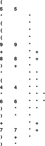
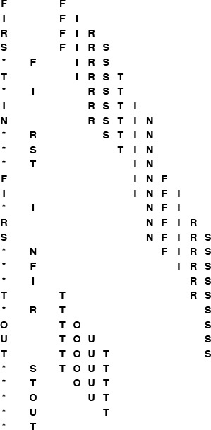
Figure 4.1 shows how a sample stack evolves through a series of push and pop operations. Each push increases the size of the stack by 1 and each pop decreases the size of the stack by 1. In the figure, the items in the stack are listed in the order that they are put on the stack, so that it is clear that the rightmost item in the list is the one at the top of the stack—the item that is to be returned if the next operation is pop. In an implementation, we are free to organize the items any way that we want, as long as we allow clients to maintain the illusion that the items are organized in this way.
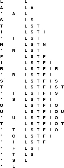
This list shows the result of the sequence of operations in the left column (top to bottom), where a letter denotes push and an asterisk denotes pop. Each line displays the operation, the letter popped for pop operations, and the contents of the stack after the operation, in order from least recently inserted to most recently inserted, left to right.
Figure 4.1 Pushdown stack (LIFO queue) example
To write programs that use the pushdown stack abstraction, we need first to define the interface. In C, one way to do so is to declare the four operations that client programs may use, as illustrated in Program 4.1. We keep these declarations in a file STACK.h that is referenced as an include file in client programs and implementations.
Furthermore, we expect that there is no other connection between client programs and implementations. We have already seen, in Chapter 1, the value of identifying the abstract operations on which a computation is based. We are now considering a mechanism that allows us to write programs that use these abstract operations. To enforce the abstraction, we hide the data structure and the implementation from the client. In Section 4.3, we consider examples of client programs that use the stack abstraction; in Section 4.4, we consider implementations.
In an ADT, the purpose of the interface is to serve as a contract between client and implementation. The function declarations ensure that the calls in the client program and the function definitions in the implementation match, but the interface otherwise contains no information about how the functions are to be implemented, or even how they are to behave. How can we explain what a stack is to a client program? For simple structures like stacks, one possibility is to exhibit the code, but this solution is clearly not effective in general. Most often, programmers resort to English-language descriptions, in documentation that accompanies the code.
A rigorous treatment of this situation requires a full description, in some formal mathematical notation, of how the functions are supposed to behave. Such a description is sometimes called a specification. Developing a specification is generally a challenging task. It has to describe any program that implements the functions in a mathematical metalanguage, whereas we are used to specifying the behavior of functions with code written in a programming language. In practice, we describe behavior in English-language descriptions. Before getting drawn further into epistemological issues, we move on. In this book, we give detailed examples, English-language descriptions, and multiple implementations for most of the ADTs that we consider.
To emphasize that our specification of the pushdown stack ADT is sufficient information for us to write meaningful client programs, we consider, in Section 4.3, two client programs that use pushdown stacks, before considering any implementation.
E A S * Y * Q U E * * * S T * * * I O * N * * *.
Give the sequence of values returned by the pop operations.
4.7 Using the conventions of Exercise 4.6, give a way to insert asterisks in the sequence E A S Y so that the sequence of values returned by the pop operations is (i) E A S Y ; (ii) Y S A E ; (iii) A S Y E ; (iv) A Y E S ; or, in each instance, prove that no such sequence exists.
![]() 4.8 Given two sequences, give an algorithm for determining whether or not asterisks can be added to make the first produce the second, when interpreted as a sequence of stack operations in the sense of Exercise 4.7.
4.8 Given two sequences, give an algorithm for determining whether or not asterisks can be added to make the first produce the second, when interpreted as a sequence of stack operations in the sense of Exercise 4.7.
4.3 Examples of Stack ADT Clients
We shall see a great many applications of stacks in the chapters that follow. As an introductory example, we now consider the use of stacks for evaluating arithmetic expressions. For example, suppose that we need to find the value of a simple arithmetic expression involving multiplication and addition of integers, such as
5 * ( ( ( 9 + 8 ) * ( 4 * 6 ) ) + 7 )
The calculation involves saving intermediate results: For example, if we calculate 9 + 8 first, then we have to save the result 17 while, say, we compute 4 * 6. A pushdown stack is the ideal mechanism for saving intermediate results in such a calculation.
We begin by considering a simpler problem, where the expression that we need to evaluate is in a form where each operator appears after its two arguments, rather than between them. As we shall see, any arithmetic expression can be arranged in this form, which is called postfix, by contrast with infix, the customary way of writing arithmetic expressions. The postfix representation of the expression in the previous paragraph is
5 9 8 + 4 6 * * 7 + *
The reverse of postfix is called prefix, or Polish notation (because it was invented by the Polish logician Lukasiewicz).
In infix, we need parentheses to distinguish, for example,
5 * ( ( ( 9 + 8 ) * ( 4 * 6 ) ) + 7 )
from
( ( 5 * 9 ) + 8 ) * ( ( 4 * 6 ) + 7 )
but parentheses are unnecessary in postfix (or prefix). To see why, we can consider the following process for converting a postfix expression to an infix expression: We replace all occurrences of two operands followed by an operator by their infix equivalent, with parentheses, to indicate that the result can be considered to be an operand. That is, we replace any occurrence of a b * and a b + by (a * b) and (a + b), respectively. Then, we perform the same transformation on the resulting expression, continuing until all the operators have been processed. For our example, the transformation happens as follows:
5 9 8 + 4 6 * * 7 + *
5 ( 9 + 8 ) ( 4 * 6 ) * 7 + *
5 ( ( 9 + 8 ) * ( 4 * 6 ) ) 7 + *
5 ( ( ( 9 + 8 ) * ( 4 * 6 ) ) + 7 ) *
( 5 * ( ( ( 9 + 8 ) * ( 4 * 6 ) ) + 7 ) )
We can determine the operands associated with any operator in the postfix expression in this way, so no parentheses are necessary.
Alternatively, with the aid of a stack, we can actually perform the operations and evaluate any postfix expression, as illustrated in Figure 4.2. Moving from left to right, we interpret each operand as the command to “push the operand onto the stack,” and each operator as the commands to “pop the two operands from the stack, perform the operation, and push the result.” Program 4.2 is a C implementation of this process.
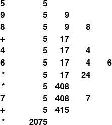
This sequence shows the use of a stack to evaluate the postfix expression 5 9 8 + 4 6 * * 7 + * . Proceeding from left to right through the expression, if we encounter a number, we push it on the stack; and if we encounter an operator, we push the result of applying the operator to the top two numbers on the stack.
Figure 4.2 Evaluation of a postfix expression
Postfix notation and an associated pushdown stack give us a natural way to organize a series of computational procedures. Some calculators and some computing languages explicitly base their method of calculation on postfix and stack operations—every operation pops its arguments from the stack and returns its results to the stack.
One example of such a language is the PostScript language, which is used to print this book. It is a complete programming language where programs are written in postfix and are interpreted with the aid of an internal stack, precisely as in Program 4.2. Although we cannot cover all the aspects of the language here (see reference section), it is sufficiently simple that we can study some actual programs, to appreciate the utility of the postfix notation and the pushdown-stack abstraction. For example, the string
5 9 8 add 4 6 mul mul 7 add mul
is a PostScript program! Programs in PostScript consist of operators (such as add and mul) and operands (such as integers). As we did in Program 4.2 we interpret a program by reading it from left to right: If we encounter an operand, we push it onto the stack; if we encounter an operator, we pop its operands (if any) from the stack and push the result (if any). Thus, the execution of this program is fully described by Figure 4.2: The program leaves the value 2075 on the stack.
PostScript has a number of primitive functions that serve as instructions to an abstract plotting device; we can also define our own functions. These functions are invoked with arguments on the stack in the same way as any other function. For example, the PostScript code
0 0 moveto 144 hill 0 72 moveto 72 hill stroke
corresponds to the sequence of actions “call moveto with arguments 0 and 0, then call hill with argument 144,” and so forth. Some operators refer directly to the stack itself. For example the operator dup duplicates the entry at the top of the stack so, for example, the PostScript code
144 dup 0 rlineto 60 rotate dup 0 rlineto
corresponds to the sequence of actions “call rlineto with arguments 144 and 0, then call rotate with argument 60, then call rlineto with arguments 144 and 0,” and so forth. The PostScript program in Figure 4.3 defines and uses the function hill. Functions in PostScript are like macros: The sequence /hill { A } def makes the name hill equivalent to the operator sequence inside the braces. Figure 4.3 is an example of a PostScript program that defines a function and draws a simple diagram.
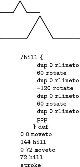
The diagram at the top was drawn by the PostScript program below it. The program is a postfix expression that uses the built-in functions moveto, rlineto, rotate, stroke and dup; and the user-defined function hill (see text). The graphics commands are instructions to a plotting device: moveto instructs that device to go to the specified position on the page (coordinates are in points, which are 1/72 inch); rlineto instructs it to move to the specified position in coordinates relative to its current position, adding the line it makes to its current path; rotate instructs it to turn left the specified number of degrees; and stroke instructs it to draw the path that it has traced.
Figure 4.3 Sample PostScript program
In the present context, our interest in PostScript is that this widely used programming language is based on the pushdown-stack abstraction. Indeed, many computers implement basic stack operations in hardware because they naturally implement a function-call mechanism: Save the current environment on entry to a function by pushing information onto a stack; restore the environment on exit by using information popped from the stack. As we see in Chapter 5, this connection between pushdown stacks and programs organized as functions that call functions is an essential paradigm of computation.
Returning to our original problem, we can also use a pushdown stack to convert fully parenthesized arithmetic expressions from infix to postfix, as illustrated in Figure 4.4. For this computation, we push the operators onto a stack, and simply pass the operands through to the output. Then, each right parenthesis indicates that both arguments for the last operator have been output, so the operator itself can be popped and output.
This sequence shows the use of a stack to convert the infix expression (5*(((9+8)*(4*6))+7)) to its postfix form 5 9 8 + 4 6 * * 7 + * . We proceed from left to right through the expression: If we encounter a number, we write it to the output; if we encounter a left parenthesis, we ignore it; if we encounter an operator, we push it on the stack; and if we encounter a right parenthesis, we write the operator at the top of the stack to the output.
Figure 4.4 Conversion of an infix expression to postfix
Program 4.3 is an implementation of this process. Note that arguments appear in the postfix expression in the same order as in the infix expression. It is also amusing to note that the left parentheses are not needed in the infix expression. The left parentheses would be required, however, if we could have operators that take differing numbers of operands (see Exercise 4.11).
In addition to providing two different examples of the use of the pushdown-stack abstraction, the entire algorithm that we have developed in this section for evaluating infix expressions is itself an exercise in abstraction. First, we convert the input to an intermediate representation (postfix). Second, we simulate the operation of an abstract stack-based machine to interpret and evaluate the expression. This same schema is followed by many modern programming-language translators, for efficiency and portability: The problem of compiling a C program for a particular computer is broken into two tasks centered around an intermediate representation, so that the problem of translating the program is separated from the problem of executing that program, just as we have done in this section. We shall see a related, but different, intermediate representation in Section 5.7.
This application also illustrates that ADTs do have their limitations. For example, the conventions that we have discussed do not provide an easy way to combine Programs 4.2 and 4.3 into a single program, using the same pushdown-stack ADT for both. Not only do we need two different stacks, but also one of the stacks holds single characters (operators), whereas the other holds numbers. To better appreciate the problem, suppose that the numbers are, say, floating-point numbers, rather than integers. Using a general mechanism to allow sharing the same implementation between both stacks (an extension of the approach that we consider in Section 4.8) is likely to be more trouble than simply using two different stacks (see Exercise 4.16). In fact, as we shall see, this solution might be the approach of choice, because different implementations may have different performance characteristics, so we might not wish to decide a priori that one ADT will serve both purposes. Indeed, our main focus is on the implementations and their performance, and we turn now to those topics for pushdown stacks.
( 5 * ( ( 9 * 8 ) + ( 7 * ( 4 + 6 ) ) ) ) .
![]() 4.10 Give, in the same manner as Figure 4.2, the contents of the stack as the following expression is evaluated by Program 4.2
4.10 Give, in the same manner as Figure 4.2, the contents of the stack as the following expression is evaluated by Program 4.2
5 9 * 8 7 4 6 + * 2 1 3 * + * + * .
![]() 4.11 Extend Programs 4.2 and 4.3 to include the
4.11 Extend Programs 4.2 and 4.3 to include the - (subtract) and / (divide) operations.
4.12 Extend your solution to Exercise 4.11 to include the unary operators - (negation) and $ (square root). Also, modify the abstract stack machine in Program 4.2 to use floating point. For example, given the expression
(-(-1) + $((-1) * (-1)-(4 * (-1))))/2
your program should print the value 1.618034.
4.13 Write a PostScript program that draws this figure:
![]() 4.14 Prove by induction that Program 4.2 correctly evaluates any postfix expression.
4.14 Prove by induction that Program 4.2 correctly evaluates any postfix expression.
![]() 4.15 Write a program that converts a postfix expression to infix, using a pushdown stack.
4.15 Write a program that converts a postfix expression to infix, using a pushdown stack.
![]() 4.16 Combine Program 4.2 and Program 4.3 into a single module that uses two different stack ADTs: a stack of integers and a stack of operators.
4.16 Combine Program 4.2 and Program 4.3 into a single module that uses two different stack ADTs: a stack of integers and a stack of operators.
![]() 4.17 Implement a compiler and interpreter for a programming language where each program consists of a single arithmetic expression preceded by a sequence of assignment statements with arithmetic expressions involving integers and variables named with single lower-case characters. For example, given the input
4.17 Implement a compiler and interpreter for a programming language where each program consists of a single arithmetic expression preceded by a sequence of assignment statements with arithmetic expressions involving integers and variables named with single lower-case characters. For example, given the input
(x = 1)
(y = (x + 1))
(((x + y) * 3) + (4 * x))
your program should print the value 13.
4.4 Stack ADT Implementations
In this section, we consider two implementations of the stack ADT: one using arrays and one using linked lists. The implementations are both straightforward applications of the basic tools that we covered in Chapter 3. They differ only, we expect, in their performance characteristics.
If we use an array to represent the stack, each of the functions declared in Program 4.1 is trivial to implement, as shown in Program 4.4. We put the items in the array precisely as diagrammed in Figure 4.1, keeping track of the index of the top of the stack. Doing the push operation amounts to storing the item in the array position indicated by the top-of-stack index, then incrementing the index; doing the pop operation amounts to decrementing the index, then returning the item that it designates. The initialize operation involves allocating an array of the indicated size, and the test if empty operation involves checking whether the index is 0. Compiled together with a client program such as Program 4.2 or Program 4.3, this implementation provides an efficient and effective pushdown stack.
We know one potential drawback to using an array representation: As is usual with data structures based on arrays, we need to know the maximum size of the array before using it, so that we can allocate memory for it. In this implementation, we make that information an argument to the function that implements initialize. This constraint is an artifact of our choice to use an array implementation; it is not an essential part of the stack ADT. We may have no easy way to estimate the maximum number of elements that our program will be putting on the stack: If we choose an arbitrarily high value, this implementation will make inefficient use of space, and that may be undesirable in an application where space is a precious resource. If we choose too small a value, our program might not work at all. By using an ADT, we make it possible to consider other alternatives, in other implementations, without changing any client program.
For example, to allow the stack to grow and shrink gracefully, we may wish to consider using a linked list, as in the implementation in Program 4.5. In this program, we keep the stack in reverse order from the array implementation, from most recently inserted element to least recently inserted element, to make the basic stack operations easier to implement, as illustrated in Figure 4.5. To pop, we remove the node from the front of the list and return its item; to push, we create a new node and add it to the front of the list. Because all linked-list operations are at the beginning of the list, we do not need to use a head node. This implementation does not need to use the argument to STACKinit.
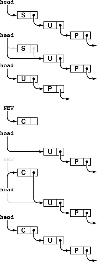
The stack is represented by a pointer head, which points to the first (most recently inserted) item. To pop the stack (top), we remove the item at the front of the list, by setting head from its link. To push a new item onto the stack (bottom), we link it in at the beginning by setting its link field to head, then setting head to point to it.
Figure 4.5 Linked-list pushdown stack
Programs 4.4 and 4.5 are two different implementations for the same ADT. We can substitute one for the other without making any changes in client programs such as the ones that we examined in Section 4.3. They differ in only their performance characteristics—the time and space that they use. For example, the list implementation uses more time for push and pop operations, to allocate memory for each push and deallocate memory for each pop. If we have an application where we perform these operations a huge number of times, we might prefer the array implementation. On the other hand, the array implementation uses the amount of space necessary to hold the maximum number of items expected throughout the computation, while the list implementation uses space proportional to the number of items, but always uses extra space for on link per item. If we need a huge stack that is usually nearly full, we might prefer the array implementation; if we have a stack whose size varies dramatically and other data structures that could make use of the space not being used when the stack has only a few items in it, we might prefer the list implementation.
These same considerations about space usage hold for many ADT implementations, as we shall see throughout the book. We often are in the position of choosing between the ability to access any item quickly but having to predict the maximum number of items needed ahead of time (in an array implementation) and the flexibility of always using space proportional to the number of items in use while giving up the ability to access every item quickly (in a linked-list implementation).
Beyond basic space-usage considerations, we normally are most interested in performance differences among ADT implementations that relate to running time. In this case, there is little difference between the two implementations that we have considered.
Property 4.1 We can implement the push and pop operations for the pushdown stack ADT in constant time, using either arrays or linked lists.
This fact follows immediately from inspection of Programs 4.4 and 4.5. ![]()
That the stack items are kept in different orders in the array and the linked-list implementations is of no concern to the client program. The implementations are free to use any data structure whatever, as long as they maintain the illusion of an abstract pushdown stack. In both cases, the implementations are able to create the illusion of an efficient abstract entity that can perform the requisite operations with just a few machine instructions. Throughout this book, our goal is to find data structures and efficient implementations for other important ADTs.
The linked-list implementation supports the illusion of a stack that can grow without bound. Such a stack is impossible in practical terms: at some point, malloc will return NULL when the request for more memory cannot be satisfied. It is also possible to arrange for an array-based stack to grow dynamically, by doubling the size of the array when the stack becomes half full, and halving the size of the array when the stack becomes half empty. We leave the details of this implementation as an exercise in Chapter 14, where we consider the process in detail for a more advanced application.
Exercises
![]() 4.18 Give the contents of
4.18 Give the contents of s[0], ..., s[4] after the execution of the operations illustrated in Figure 4.1, using Program 4.4.
![]() 4.19 Suppose that you change the pushdown-stack interface to replace test if empty by count, which should return the number of items currently in the data structure. Provide implementations for count for the array representation (Program 4.4) and the linked-list representation (Program 4.5).
4.19 Suppose that you change the pushdown-stack interface to replace test if empty by count, which should return the number of items currently in the data structure. Provide implementations for count for the array representation (Program 4.4) and the linked-list representation (Program 4.5).
4.20 Modify the array-based pushdown-stack implementation in the text (Program 4.4) to call a function STACKerror if the client attempts to pop when the stack is empty or to push when the stack is full.
4.21 Modify the linked-list–based pushdown-stack implementation in the text (Program 4.5) to call a function STACKerror if the client attempts to pop when the stack is empty or if there is no memory available from malloc for a push.
4.22 Modify the linked-list–based pushdown-stack implementation in the text (Program 4.5) to use an array of indices to implement the list (see Figure 3.4).
4.23 Write a linked-list–based pushdown-stack implementation that keeps items on the list in order from least recently inserted to most recently inserted. You will need to use a doubly linked list.
![]() 4.24 Develop an ADT that provides clients with two different pushdown stacks. Use an array implementation. Keep one stack at the beginning of the array and the other at the end. (If the client program is such that one stack grows while the other one shrinks, this implementation uses less space than other alternatives.)
4.24 Develop an ADT that provides clients with two different pushdown stacks. Use an array implementation. Keep one stack at the beginning of the array and the other at the end. (If the client program is such that one stack grows while the other one shrinks, this implementation uses less space than other alternatives.)
![]() 4.25 Implement an infix-expression–evaluation function for integers that includes Programs 4.2 and 4.3, using your ADT from Exercise 4.24.
4.25 Implement an infix-expression–evaluation function for integers that includes Programs 4.2 and 4.3, using your ADT from Exercise 4.24.
4.5 Creation of a New ADT
Sections 4.2 through 4.4 present a complete example of C code that captures one of our most important abstractions: the pushdown stack. The interface in Section 4.2 defines the basic operations; client programs such as those in Section 4.3 can use those operations without dependence on how the operations are implemented; and implementations such as those in Section 4.4 provide the necessary concrete representation and program code to realize the abstraction.
To design a new ADT, we often enter into the following process. Starting with the task of developing a client program to solve an applications problem, we identify operations that seem crucial: What would we like to be able to do with our data? Then, we define an interface and write client code to test the hypothesis that the existence of the ADT would make it easier for us to implement the client program. Next, we consider the idea of whether or not we can implement the operations in the ADT with reasonable efficiency. If we cannot, we perhaps can seek to understand the source of the inefficiency and to modify the interface to include operations that are better suited to efficient implementation. These modifications affect the client program, and we modify it accordingly. After a few iterations, we have a working client program and a working implementation, so we freeze the interface: We adopt a policy of not changing it. At this moment, the development of client programs and the development of implementations are separable: We can write other client programs that use the same ADT (perhaps we write some driver programs that allow us to test the ADT), we can write other implementations, and we can compare the performance of multiple implementations.
In other situations, we might define the ADT first. This approach might involve asking questions such as these: What basic operations would client programs want to perform on the data at hand? Which operations do we know how to implement efficiently? After we develop an implementation, we might test its efficacy on client programs. We might modify the interface and do more tests, before eventually freezing the interface.
In Chapter 1, we considered a detailed example where thinking on an abstract level helped us to find an efficient algorithm for solving a complex problem. We consider next the use of the general approach that we are discussing in this chapter to encapsulate the specific abstract operations that we exploited in Chapter 1.
Program 4.6 defines the interface, in terms of two operations (in addition to initialize) that seem to characterize the algorithms that we considered in Chapter 1 for connectivity, at a high abstract level. Whatever the underlying algorithms and data structures, we want to be able to check whether or not two nodes are known to be connected, and to declare that two nodes are connected.
Program 4.7 is a client program that uses the ADT defined in the interface of Program 4.6 to solve the connectivity problem. One benefit of using the ADT is that this program is easy to understand, because it is written in terms of abstractions that allow the computation to be expressed in a natural way.
Program 4.8 is an implementation of the union–find interface defined in Program 4.6 that uses a forest of trees represented by two arrays as the underlying representation of the known connectivity information, as described in Section 1.3. The different algorithms that we considered in Chapter 1 represent different implementations of this ADT, and we can test them as such without changing the client program at all.
This ADT leads to programs that are slightly less efficient than those in Chapter 1 for the connectivity application, because it does not take advantage of the property of that client that every union operation is immediately preceded by a find operation. We sometimes incur extra costs of this kind as the price of moving to a more abstract representation. In this case, there are numerous ways to remove the inefficiency, perhaps at the cost of making the interface or the implementation more complicated (see Exercise 4.27). In practice, the paths are extremely short (particularly if we use path compression), so the extra cost is likely to be negligible in this case.
The combination of Programs 4.6 through 4.8 is operationally equivalent to Program 1.3, but splitting the program into three parts is a more effective approach because it
• Separates the task of solving the high-level (connectivity) problem from the task of solving the low-level (union–find) problem, allowing us to work on the two problems independently
• Gives us a natural way to compare different algorithms and data structures for solving the problem
• Gives us an abstraction that we can use to build other algorithms
• Defines, through the interface, a way to check that the software is operating as expected
• Provides a mechanism that allows us to upgrade to new representations (new data structures or new algorithms) without changing the client program at all
These benefits are widely applicable to many tasks that we face when developing computer programs, so the basic tenets underlying ADTs are widely used.
Exercises
4.26 Modify Program 4.8 to use path compression by halving.
4.27 Remove the inefficiency mentioned in the text by adding an operation to Program 4.6 that combines union and find, providing an implementation in Program 4.8, and modifying Program 4.7 accordingly.
![]() 4.28 Modify the interface (Program 4.6) and implementation (Program 4.8) to provide a function that will return the number of nodes known to be connected to a given node.
4.28 Modify the interface (Program 4.6) and implementation (Program 4.8) to provide a function that will return the number of nodes known to be connected to a given node.
4.29 Modify Program 4.8 to use an array of structures instead of parallel arrays for the underlying data structure.
4.6 FIFO Queues and Generalized Queues
The first-in, first-out (FIFO) queue is another fundamental ADT that is similar to the pushdown stack, but that uses the opposite rule to decide which element to remove for delete. Rather than removing the most recently inserted element, we remove the element that has been in the queue the longest.
Perhaps our busy professor’s “in” box should operate like a FIFO queue, since the first-in, first-out order seems to be an intuitively fair way to decide what to do next. However, that professor might not ever answer the phone or get to class on time! In a stack, a memorandum can get buried at the bottom, but emergencies are handled when they arise; in a FIFO queue, we work methodically through the tasks, but each has to wait its turn.
FIFO queues are abundant in everyday life. When we wait in line to see a movie or to buy groceries, we are being processed according to a FIFO discipline. Similarly, FIFO queues are frequently used within computer systems to hold tasks that are yet to be accomplished when we want to provide services on a first-come, first-served basis. Another example, which illustrates the distinction between stacks and FIFO queues, is a grocery store’s inventory of a perishable product. If the grocer puts new items on the front of the shelf and customers take items from the front, then we have a stack discipline, which is a problem for the grocer because items at the back of the shelf may stay there for a very long time and therefore spoil. By putting new items at the back of the shelf, the grocer ensures that the length of time any item has to stay on the shelf is limited by the length of time it takes customers to purchase the maximum number of items that fit on the shelf. This same basic principle applies to numerous similar situations.
Definition 4.3 A FIFO queue is an ADT that comprises two basic operations: insert (put) a new item, and delete (get) the item that was least recently inserted.
Program 4.9 is the interface for a FIFO queue ADT. This interface differs from the stack interface that we considered in Section 4.2 only in the nomenclature: to a compiler, say, the two interfaces are identical! This observation underscores the fact that the abstraction itself, which programmers normally do not define formally, is the essential component of an ADT. For large applications, which may involve scores of ADTs, the problem of defining them precisely is critical. In this book, we work with ADTs that capture essential concepts that we define in the text, but not in any formal language, other than via specific implementations. To discern the nature of ADTs, we need to consider examples of their use and to examine specific implementations.
Figure 4.6 shows how a sample FIFO queue evolves through a series of get and put operations. Each get decreases the size of the queue by 1 and each put increases the size of the queue by 1. In the figure, the items in the queue are listed in the order that they are put on the queue, so that it is clear that the first item in the list is the one that is to be returned by the get operation. Again, in an implementation, we are free to organize the items any way that we want, as long as we maintain the illusion that the items are organized in this way.
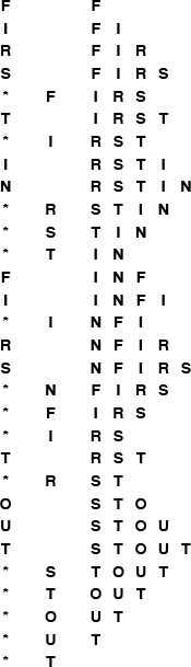
This list shows the result of the sequence of operations in the left column (top to bottom), where a letter denotes put and an asterisk denotes get. Each line displays the operation, the letter returned for get operations, and the contents of the queue in order from least recently inserted to most recently inserted, left to right.
Figure 4.6 FIFO queue example
To implement the FIFO queue ADT using a linked list, we keep the items in the list in order from least recently inserted to most recently inserted, as diagrammed in Figure 4.6. This order is the reverse of the order that we used for the stack implementation, but allows us to develop efficient implementations of the queue operations. We maintain two pointers into the list: one to the beginning (so that we can get the first element), and one to the end (so that we can put a new element onto the queue), as shown in Figure 4.7 and in the implementation in Program 4.10.
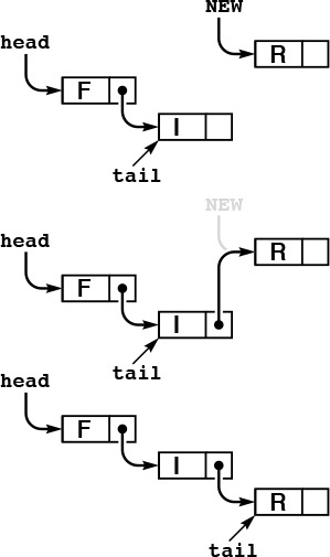
In this linked-list representation of a queue, we insert new items at the end, so the items in the linked list are in order from least recently inserted to most recently inserted, from beginning to end. The queue is represented by two pointers head and tail which point to the first and final item, respectively. To get an item from the queue, we remove the item at the front of the list, in the same way as we did for stacks (see Figure 4.5). To put a new item onto the queue, we set the link field of the node referenced by tail to point to it (center), then update tail (bottom).
Figure 4.7 Linked-list queue
We can also use an array to implement a FIFO queue, although we have to exercise care to keep the running time constant for both the put and get operations. That performance goal dictates that we can not move the elements of the queue within the array, unlike what might be suggested by a literal interpretation of Figure 4.6. Accordingly, as we did with the linked-list implementation, we maintain two indices into the array: one to the beginning of the queue and one to the end of the queue. We consider the contents of the queue to be the elements between the indices. To get an element, we remove it from the beginning (head) of the queue and increment the head index; to put an element, we add it to the end (tail) of the queue and increment the tail index. A sequence of put and get operations causes the queue to appear to move through the array, as illustrated in Figure 4.8. When it hits the end of the array, we arrange for it to wrap around to the beginning. The details of this computation are in the code in Program 4.11.
This sequence shows the data manipulation underlying the abstract representation in Figure 4.6 when we implement the queue by storing the items in an array, keeping indices to the beginning and end of the queue, and wrapping the indices back to the beginning of the array when they reach the end of the array. In this example, the tail index wraps back to the beginning when the second T is inserted, and the head index wraps when the second S is removed.
Figure 4.8 FIFO queue example, array implementation
Property 4.2 We can implement the get and put operations for the FIFO queue ADT in constant time, using either arrays or linked lists.
This fact is immediately clear when we inspect the code in Programs 4.10 and 4.11. ![]()
The same considerations that we discussed in Section 4.4 apply to space resources used by FIFO queues. The array representation requires that we reserve enough space for the maximum number of items expected throughout the computation, whereas the linked-list representation uses space proportional to the number of elements in the data structure, at the cost of extra space for the links and extra time to allocate and deallocate memory for each operation.
Although we encounter stacks more often than we encounter FIFO queues, because of the fundamental relationship between stacks and recursive programs (see Chapter 5), we shall also encounter algorithms for which the queue is the natural underlying data structure. As we have already noted, one of the most frequent uses of queues and stacks in computational applications is to postpone computation. Although many applications that involve a queue of pending work operate correctly no matter what rule is used for delete, the overall running time or other resource usage may be dependent on the rule. When such applications involve a large number of insert and delete operations on data structures with a large number of items on them, performance differences are paramount. Accordingly, we devote a great deal of attention in this book to such ADTs. If we ignored performance, we could formulate a single ADT that encompassed insert and delete; since we do not ignore performance, each rule, in essence, constitutes a different ADT. To evaluate the effectiveness of a particular ADT, we need to consider two costs: the implementation cost, which depends on our choice of algorithm and data structure for the implementation; and the cost of the particular decision-making rule in terms of effect on the performance of the client. To conclude this section, we will describe a number of such ADTs, which we will be considering in detail throughout the book.
Specifically, pushdown stacks and FIFO queues are special instances of a more general ADT: the generalized queue. Instances of generalized queues differ in only the rule used when items are removed. For stacks, the rule is “remove the item that was most recently inserted”; for FIFO queues, the rule is “remove the item that was least recently inserted”; and there are many other possibilities, a few of which we now consider.
A simple but powerful alternative is the random queue, where the rule is to “remove a random item,” and the client can expect to get any of the items on the queue with equal probability. We can implement the operations of a random queue in constant time using an array representation (see Exercise 4.42). As do stacks and FIFO queues, the array representation requires that we reserve space ahead of time. The linked-list alternative is less attractive than it was for stacks and FIFO queues, however, because implementing both insertion and deletion efficiently is a challenging task (see Exercise 4.43). We can use random queues as the basis for randomized algorithms, to avoid, with high probability, worst-case performance scenarios (see Section 2.7).
We have described stacks and FIFO queues by identifying items according to the time that they were inserted into the queue. Alternatively, we can describe these abstract concepts in terms of a sequential listing of the items in order, and refer to the basic operations of inserting and deleting items from the beginning and the end of the list. If we insert at the end and delete at the end, we get a stack (precisely as in our array implementation); if we insert at the beginning and delete at the beginning, we also get a stack (precisely as in our linked-list implementation); if we insert at the end and delete at the beginning, we get a FIFO queue (precisely as in our linked-list implementation); and if we insert at the beginning and delete at the end, we also get a FIFO queue (this option does not correspond to any of our implementations—we could switch our array implementation to implement it precisely, but the linked-list implementation is not suitable because of the need to back up the pointer to the end when we remove the item at the end of the list). Building on this point of view, we are led to the deque ADT, where we allow either insertion or deletion at either end. We leave the implementations for exercises (see Exercises 4.37 through 4.41), noting that the array-based implementation is a straightforward extension of Program 4.11, and that the linked-list implementation requires a doubly linked list, unless we restrict the deque to allow deletion at only one end.
In Chapter 9, we consider priority queues, where the items have keys and the rule for deletion is “remove the item with the smallest key.” The priority-queue ADT is useful in a variety of applications, and the problem of finding efficient implementations for this ADT has been a research goal in computer science for many years. Identifying and using the ADT in applications has been an important factor in this research: we can get an immediate indication whether or not a new algorithm is correct by substituting its implementation for an old implementation in a huge, complex application and checking that we get the same result. Moreover, we get an immediate indication whether a new algorithm is more efficient than an old one by noting the extent to which substituting the new implementation improves the overall running time. The data structures and algorithms that we consider in Chapter 9 for solving this problem are interesting, ingenious, and effective.
In Chapters 12 through 16, we consider symbol tables, which are generalized queues where the items have keys and the rule for deletion is “remove an item whose key is equal to a given key, if there is one.” This ADT is perhaps the most important one that we consider, and we shall examine dozens of implementations.
Each of these ADTs also give rise to a number of related, but different, ADTs that suggest themselves as an outgrowth of careful examination of client programs and the performance of implementations. In Sections 4.7 and 4.8, we consider numerous examples of changes in the specification of generalized queues that lead to yet more different ADTs, which we shall consider later in this book.
Exercises
![]() 4.30 Give the contents of
4.30 Give the contents of q[0], ..., q[4] after the execution of the operations illustrated in Figure 4.6, using Program 4.11. Assume that maxN is 10, as in Figure 4.8.
![]() 4.31 A letter means put and an asterisk means get in the sequence
4.31 A letter means put and an asterisk means get in the sequence
E A S * Y * Q U E * * * S T * * * I O * N * * *.
Give the sequence of values returned by the get operations when this sequence of operations is performed on an initially empty FIFO queue.
4.32 Modify the array-based FIFO queue implementation in the text (Program 4.11) to call a function QUEUEerror if the client attempts to get when the queue is empty or to put when the queue is full.
4.33 Modify the linked-list–based FIFO queue implementation in the text (Program 4.10) to call a function QUEUEerror if the client attempts to get when the queue is empty or if there is no memory available from malloc for a put.
![]() 4.34 An uppercase letter means put at the beginning, a lowercase letter means put at the end, a plus sign means get from the beginning, and an asterisk means get from the end in the sequence
4.34 An uppercase letter means put at the beginning, a lowercase letter means put at the end, a plus sign means get from the beginning, and an asterisk means get from the end in the sequence
E A s + Y + Q U E * * + s t + * + I O * n + + *.
Give the sequence of values returned by the get operations when this sequence of operations is performed on an initially empty deque.
![]() 4.35 Using the conventions of Exercise 4.34, give a way to insert plus signs and asterisks in the sequence E a s Y so that the sequence of values returned by the get operations is (i) E s a Y ; (ii) Y a s E ; (iii) a Y s E ; (iv) a s Y E ; or, in each instance, prove that no such sequence exists.
4.35 Using the conventions of Exercise 4.34, give a way to insert plus signs and asterisks in the sequence E a s Y so that the sequence of values returned by the get operations is (i) E s a Y ; (ii) Y a s E ; (iii) a Y s E ; (iv) a s Y E ; or, in each instance, prove that no such sequence exists.
![]() 4.36 Given two sequences, give an algorithm for determining whether or not it is possible to add plus signs and asterisks to make the first produce the second when interpreted as a sequence of deque operations in the sense of Exercise 4.35.
4.36 Given two sequences, give an algorithm for determining whether or not it is possible to add plus signs and asterisks to make the first produce the second when interpreted as a sequence of deque operations in the sense of Exercise 4.35.
![]() 4.37 Write an interface for the deque ADT.
4.37 Write an interface for the deque ADT.
4.38 Provide an implementation for your deque interface (Exercise 4.37) that uses an array for the underlying data structure.
4.39 Provide an implementation for your deque interface (Exercise 4.37) that uses a doubly linked list for the underlying data structure.
4.40 Provide an implementation for the FIFO queue interface in the text (Program 4.9) that uses a circular list for the underlying data structure.
4.41 Write a client that tests your deque ADTs (Exercise 4.37) by reading, as the first argument on the command line, a string of commands like those given in Exercise 4.34 then performing the indicated operations. Add a function DQdump to the interface and implementations, and print out the contents of the deque after each operation, in the style of Figure 4.6.
![]() 4.42 Build a random-queue ADT by writing an interface and an implementation that uses an array as the underlying data structure. Make sure that each operation takes constant time.
4.42 Build a random-queue ADT by writing an interface and an implementation that uses an array as the underlying data structure. Make sure that each operation takes constant time.
![]() 4.43 Build a random-queue ADT by writing an interface and an implementation that uses a linked list as the underlying data structure. Provide implementations for insert and delete that are as efficient as you can make them, and analyze their worst-case cost.
4.43 Build a random-queue ADT by writing an interface and an implementation that uses a linked list as the underlying data structure. Provide implementations for insert and delete that are as efficient as you can make them, and analyze their worst-case cost.
![]() 4.44 Write a client that picks numbers for a lottery by putting the numbers 1 through 99 on a random queue, then prints the result of removing five of them.
4.44 Write a client that picks numbers for a lottery by putting the numbers 1 through 99 on a random queue, then prints the result of removing five of them.
4.45 Write a client that takes an integer N from the first argument on the command line, then prints out N poker hands, by putting N items on a random queue (see Exercise 4.4), then printing out the result of picking five cards at a time from the queue.
![]() 4.46 Write a program that solves the connectivity problem by inserting all the pairs on a random queue and then taking them from the queue, using the quick-find–weighted algorithm (Program 1.3).
4.46 Write a program that solves the connectivity problem by inserting all the pairs on a random queue and then taking them from the queue, using the quick-find–weighted algorithm (Program 1.3).
4.7 Duplicate and Index Items
For many applications, the abstract items that we process are unique, a quality that leads us to consider modifying our idea of how stacks, FIFO queues, and other generalized ADTs should operate. Specifically, in this section, we consider the effect of changing the specifications of stacks, FIFO queues, and generalized queues to disallow duplicate items in the data structure.
For example, a company that maintains a mailing list of customers might want to try to grow the list by performing insert operations from other lists gathered from many sources, but would not want the list to grow for an insert operation that refers to a customer already on the list. We shall see that the same principle applies in a variety of applications. For another example, consider the problem of routing a message through a complex communications network. We might try going through several paths simultaneously in the network, but there is only one message, so any particular node in the network would want to have only one copy in its internal data structures.
One approach to handling this situation is to leave up to the clients the task of ensuring that duplicate items are not presented to the ADT, a task that clients presumably might carry out using some different ADT. But since the purpose of an ADT is to provide clients with clean solutions to applications problems, we might decide that detecting and resolving duplicates is a part of the problem that the ADT should help to solve.
The policy of disallowing duplicate items is a change in the abstraction: the interface, names of the operations, and so forth for such an ADT are the same as those for the corresponding ADT without the policy, but the behavior of the implementation changes in a fundamental way. In general, whenever we modify the specification of an ADT, we get a completely new ADT—one that has completely different properties. This situation also demonstrates the precarious nature of ADT specification: Being sure that clients and implementations adhere to the specifications in an interface is difficult enough, but enforcing a high-level policy such as this one is another matter entirely. Still, we are interested in algorithms that do so because clients can exploit such properties to solve problems in new ways, and implementations can take advantage of such restrictions to provide more efficient solutions.
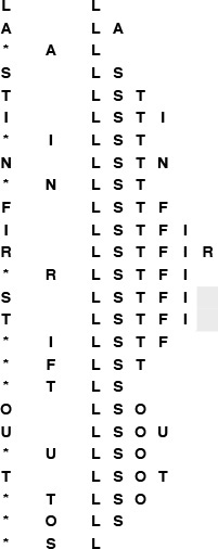
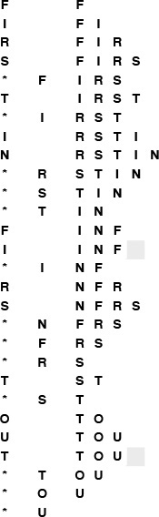
Figure 4.9 shows how a modified no-duplicates stack ADT would operate for the example corresponding to Figure 4.1; Figure 4.10 shows the effect of the change for FIFO queues.
This sequence shows the result of the same operations as those in Figure 4.1, but for a stack with no duplicate objects allowed. The gray squares mark situations where the stack is left unchanged because the item to be pushed is already on the stack. The number of items on the stack is limited by the number of possible distinct items.
Figure 4.9 Pushdown stack with no duplicates
This sequence shows the result of the same operations as those in Figure 4.6, but for a queue with no duplicate objects allowed. The gray squares mark situations where the queue is left unchanged because the item to be put onto the queue is already there.
Figure 4.10 FIFO queue with no duplicates, ignore-the-new-item policy
In general, we have a policy decision to make when a client makes an insert request for an item that is already in the data structure. Should we proceed as though the request never happened, or should we proceed as though the client had performed a delete followed by an insert? This decision affects the order in which items are ultimately processed for ADTs such as stacks and FIFO queues (see Figure 4.11), and the distinction is significant for client programs. For example, the company using such an ADT for a mailing list might prefer to use the new item (perhaps assuming that it has more up-to-date information about the customer), and the switching mechanism using such an ADT might prefer to ignore the new item (perhaps it has already taken steps to send along the message). Furthermore, this policy choice affects the implementations: the forget-the-old-item policy is generally more difficult to implement than the ignore-the-new-item policy, because it requires that we modify the data structure.
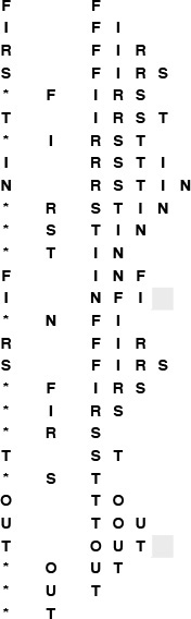
This sequence shows the result of the same operations as in Figure 4.10, but using the (more difficult to implement) policy by which we always add a new item at the end of the queue. If there is a duplicate, we remove it.
Figure 4.11 FIFO queue with no duplicates, forget-the-old-item policy
To implement generalized queues with no duplicate items, we assume that we have an abstract operation for testing item equality, as discussed in Section 4.1. Given such an operation, we still need to be able to determine whether a new item to be inserted is already in the data structure. This general case amounts to implementing the symbol table ADT, so we shall consider it in the context of the implementations given in Chapters 12 through 15.
There is an important special case for which we have a straightforward solution, which is illustrated for the pushdown stack ADT in Program 4.12. This implementation assumes that the items are integers in the range 0 to M − 1. Then, it uses a second array, indexed by the item itself, to determine whether that item is in the stack. When we insert item i, we set the ith entry in the second array to 1; when we delete item i, we set the ith entry in the array to 0. Otherwise, we use the same code as before to insert and delete items, with one additional test: Before inserting an item, we can test to see whether it is already in the stack. If it is, we ignore the push. This solution does not depend on whether we use an array or linked-list (or some other) representation for the stack. Implementing an ignore-the-old-item policy involves more work (see Exercise 4.51).
In summary, one way to implement a stack with no duplicates using an ignore-the-new-item policy is to maintain two data structures: the first contains the items in the stack, as before, to keep track of the order in which the items in the stack were inserted; the second is an array that allows us to keep track of which items are in the stack, by using the item as an index. Using an array in this way is a special case of a symbol-table implementation, which is discussed in Section 12.2. We can apply the same technique to any generalized queue ADT, when we know the items to be integers in the range 0 to M – 1.
This special case arises frequently. The most important example is when the items in the data structure are themselves array indices, so we refer to such items as index items. Typically, we have a set of M objects, kept in yet another array, that we need to pass through a generalized queue structure as a part of a more complex algorithm. Objects are put on the queue by index and processed when they are removed, and each object is to be processed precisely once. Using array indices in a queue with no duplicates accomplishes this goal directly.
Each of these choices (disallow duplicates, or do not; and use the new item, or do not) leads to a new ADT. The differences may seem minor, but they obviously affect the dynamic behavior of the ADT as seen by client programs, and affect our choice of algorithm and data structure to implement the various operations, so we have no alternative but to treat all the ADTs as different. Furthermore, we have other options to consider: For example, we might wish to modify the interface to inform the client program when it attempts to insert a duplicate item, or to give the client the option whether to ignore the new item or to forget the old one.
When we informally use a term such as pushdown stack, FIFO queue, deque, priority queue, or symbol table, we are potentially referring to a family of ADTs, each with different sets of defined operations and different sets of conventions about the meanings of the operations, each requiring different and, in some cases, more sophisticated implementations to be able to support those operations efficiently.
Exercises
![]() 4.47 Draw a figure corresponding to Figure 4.9 for the stack ADT that disallows duplicates using a forget-the-old-item policy.
4.47 Draw a figure corresponding to Figure 4.9 for the stack ADT that disallows duplicates using a forget-the-old-item policy.
4.48 Modify the standard array-based stack implementation in Section 4.4 (Program 4.4) to disallow duplicates with an ignore-the-new-item policy. Use a brute-force approach that involves scanning through the whole stack.
4.49 Modify the standard array-based stack implementation in Section 4.4 (Program 4.4) to disallow duplicates with a forget-the-old-item policy. Use a brute-force approach that involves scanning through, and possibly rearranging, the whole stack.
![]() 4.50 Do Exercises 4.48 and 4.49 for the linked-list–based stack implementation in Section 4.4 (Program 4.5).
4.50 Do Exercises 4.48 and 4.49 for the linked-list–based stack implementation in Section 4.4 (Program 4.5).
![]() 4.51 Develop a pushdown-stack implementation that disallows duplicates, using a forget-the-old-item policy for integer items between 0 and M – 1, and that uses constant time for both push and pop. Hint: Use a doubly linked list representation for the stack and keep pointers to nodes, rather than 0–1 values, in an item-indexed array.
4.51 Develop a pushdown-stack implementation that disallows duplicates, using a forget-the-old-item policy for integer items between 0 and M – 1, and that uses constant time for both push and pop. Hint: Use a doubly linked list representation for the stack and keep pointers to nodes, rather than 0–1 values, in an item-indexed array.
4.52 Do Exercises 4.48 and 4.49 for the FIFO queue ADT.
4.53 Do Exercise 4.50 for the FIFO queue ADT.
4.54 Do Exercise 4.51 for the FIFO queue ADT.
4.55 Do Exercises 4.48 and 4.49 for the randomized-queue ADT.
4.56 Write a client program for your ADT from Exercise 4.55, which exercises a randomized queue with no duplicates.
4.8 First-Class ADTs
Our interfaces and implementations of stack and FIFO queue ADTs in Sections 4.2 through 4.7 provide clients with the capability to use a single instance of a particular generalized stack or queue, and to achieve the important objective of hiding from the client the particular data structure used in the implementation. Such ADTs are widely useful, and will serve as the basis for many of the implementations that we consider in this book.
These objects are disarmingly simple when considered as ADTs themselves, however, because there is only one object in a given program. The situation is analogous to having a program, for example, that manipulates only one integer. We could perhaps increment, decrement, and test the value of the integer, but could not declare variables or use it as an argument or return value in a function, or even multiply it by another integer. In this section, we consider how to construct ADTs that we can manipulate in the same way that we manipulate built-in types in client programs, while still achieving the objective of hiding the implementation from the client.
Definition 4.4 A first-class data type is one for which we can have potentially many different instances, and which we can assign to variables which we can declare to hold the instances.
For example, we could use first-class data types as arguments and return values to functions.
The method that we will use to implement first-class data types applies to any data type: in particular, it applies to generalized queues, so it provides us with the capability to write programs that manipulate stacks and FIFO queues in much the same way that we manipulate other types of data in C. This capability is important in the study of algorithms because it provides us with a natural way to express high-level operations involving such ADTs. For example, we can speak of operations to join two queues—to combine them into one. We shall consider algorithms that implement such operations for the priority queue ADT (Chapter 9) and for the symbol table ADT (Chapter 12).
Some modern languages provide specific mechanisms for building first-class ADTs, but the idea transcends specific mechanisms. Being able to manipulate instances of ADTs in much the same way that we manipulate built-in data types such as int or float is an important goal in the design of many high-level programming languages, because it allows any applications program to be written such that the program manipulates the objects of central concern to the application; it allows many programmers to work simultaneously on large systems, all using a precisely defined set of abstract operations; and it provides for those abstract operations to be implemented in many different ways without any changes to the applications code—for example for new machines and programming environments. Some languages even allow operator overloading, which allows us to use basic symbols such as + or * to define operators. C does not provide specific support for building first-class data types, but it does provide primitive operations that we can use to achieve that goal. There are a number of ways to proceed in C. To keep our focus on algorithms and data structures, as opposed to programming-language design issues, we do not consider all the alternatives; rather, we describe and adopt just one convention that we can use throughout the book.
To illustrate the basic approach, we begin by considering, as an example, a first-class data type and then a first-class ADT for the complex-number abstraction. Our goal is to be able to write programs like Program 4.13, which performs algebraic operations on complex numbers using operations defined in the ADT. We implement the add and multiply operations as standard C functions, since C does not support operator overloading.
Program 4.13 uses few properties of complex numbers; we now digress to consider these properties briefly. In one sense, we are not digressing at all, because it is interesting to contemplate the relationship between complex numbers themselves as a mathematical abstraction and this abstract representation of them in a computer program.
The number ![]() is an imaginary number. Although
is an imaginary number. Although ![]() is meaningless as a real number, we name it i, and perform algebraic manipulations with i, replacing i2 with –1 whenever it appears. A complex number consists of two parts, real and imaginary—complex numbers can be written in the form a + bi, where a and b are reals. To multiply complex numbers, we apply the usual algebraic rules, replacing i2 with –1 whenever it appears. For example,
is meaningless as a real number, we name it i, and perform algebraic manipulations with i, replacing i2 with –1 whenever it appears. A complex number consists of two parts, real and imaginary—complex numbers can be written in the form a + bi, where a and b are reals. To multiply complex numbers, we apply the usual algebraic rules, replacing i2 with –1 whenever it appears. For example,
(a + bi)(c + di) = ac + bci + adi + bdi2 = (ac – bd) + (ad + bc)i.
The real or imaginary parts might cancel out (have the value 0) when we perform a complex multiplication. For example,
(1 – i)(1 – i) = 1 – i – i + i2 = –2i,
(1 + i)4 = 4i2 = –4,
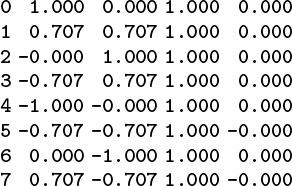
This table gives the output that is produced by Program 4.13 when invoked with a.out 8. The eight complex roots of unity are ±1, ±i, and
(left two columns). Each of these eight numbers gives the result 1 + 0i when raised to the eighth power (right two columns).
Figure 4.12 Complex roots of unity
(1 + i)8 = 16.
Scaling the preceding equation by dividing through by ![]() , we find that
, we find that
In general, there are many complex numbers that evaluate to 1 when raised to a power. These are the complex roots of unity. Indeed, for each N, there are exactly N complex numbers z with zN = 1. The numbers
for k = 0, 1, ..., N – 1 are easily shown to have this property (see Exercise 4.63). For example, taking k = 1 and N = 8 in this formula gives the particular eighth root of unity that we just discovered.
Program 4.13 is an example of a client program for the complex-numbers ADT that raises each of the Nth roots of unity to the Nth power, using the multiplication operation defined in the ADT. The output that it produces in shown in Figure 4.12: We expect that each number raised to the Nth power gives the same result: 1, or 1 + 0i.
This client program differs from the client programs that we have considered to this point in one major respect: it declares variables of type Complex and assigns values to such variables, including using them as arguments and return values in functions. Accordingly, we need to define the type Complex in the interface.
Program 4.14 is an interface for complex numbers that we might consider using. It defines the type Complex as a struct comprising two floats (for the real and imaginary part of the complex number), and declares four functions for processing complex numbers: initialize, extract real and imaginary parts, and multiply. Program 4.15 gives implementations of these functions, which are straightforward. Together, these two functions provide an effective implementation of a complex-number ADT that we can use successfully in client programs such as Program 4.13.
The interface in Program 4.14 specifies one particular representation for complex numbers—a structure containing two integers (the real and imaginary parts). By including this representation within the interface, however, we are making it available for use by client programs. Programmers often organize interfaces in this way. Essentially, doing so amounts to publishing a standard representation for a new data type that might be used by many client programs. In this example, client programs could refer directly to t.Re and t.Im for any variable t of type Complex. The advantage of allowing such access is that we thus ensure that clients that need to directly implement their own manipulations that may not be present in the type’s suite of operations at least agree on the standard representation. The disadvantage of allowing clients direct access to the data is that we cannot change the representation without changing all the clients. In short, Program 4.14 is not an abstract data type, because the representation is not hidden by the interface.
Even for this simple example, the difficulty of changing representations is significant because there is another standard representation that we might wish to consider using: polar coordinates (see Exercise 4.62). For an application with more complicated data structures, the ability to change representations is a requirement. For example, our company that needs to process mailing lists needs to use the same client program to process mailing lists in different formats. With a first-class ADT, the client programs can manipulate the data without direct access, but rather with indirect access, through operations defined in the ADT. An operation such as extract customer name then can have different implementations for different list formats. The most important implication of this arrangement is that we can change the data representation without having to change the client programs.
We use the term handle to describe a reference to an abstract object. Our goal is to give client programs handles to abstract objects that can be used in assignment statements and as arguments and return values of functions in the same way as built-in data types, while hiding the representation of the objects from the client program.
Program 4.16 is an example of such an interface for complex numbers that achieves this goal, and exemplifies the conventions that we shall use throughout this book. The handle is defined as a pointer to a structure that has a name tag, but is otherwise not specified. The client can use this handle as intended, but there can be no code in the client program that uses the handle in any other way: It cannot access a field in a structure by dereferencing the pointer because it does not have the names of any of the fields. In the interface, we define functions which accept handles as arguments and also return handles as values; and client programs can use those functions, all without knowing anything about the data structure that will be used to implement the interface.
Program 4.17 is an implementation of the interface of Program 4.16. It defines the specific data structure that will be used to implement handles and the data type itself; a function that allocates the memory for a new object and initializes its fields; functions that provide access to the fields (which we implement by dereferencing the handle pointer to access the specific fields in the argument objects); and functions that implement the ADT operations. All information specific to the data structure being used is guaranteed to be encapsulated in the implementation, because the client has no way to refer to it.
The distinction between the data type for complex numbers in the code in Programs 4.14 and 4.15 and the ADT for complex numbers in the code in Programs 4.16 and 4.17 is essential and is thus well worth careful study. It is a mechanism that we can use to develop and compare efficient algorithms for fundamental problems throughout this book. We shall not treat all the implications of using such a mechanism for software engineering in further detail, but it is a powerful and general mechanism that will serve us well in the study of algorithms and data structures and their application.
In particular, the issue of storage management is critical in the use of ADTs in software engineering. When we say x = t in Program 4.13, where the variables are both of type Complex, we simply are assigning a pointer. The alternative would be to allocate memory for a new object and define an explicit copy function to copy the values in the object associated with t to the new object. This issue of copy semantics is an important one to address in any ADT design. We normally use pointer assignment (and therefore do not consider copy implementations for our ADTs) because of our focus on efficiency—this choice makes us less susceptible to excessive hidden costs when performing operations on huge data structures. The design of the C string data type is based on similar considerations.
The implementation of COMPLEXmult in Program 4.15 creates a new object for the result. Alternatively, more in the spirit of reserving explicit object-creation operations for the client, we could return the value in one of the arguments. As it stands, COMPLEXmult has a defect called a memory leak, that makes the program unusable for a huge number of multiplications. The problem is that each multiplication allocates memory for a new object, but we never execute any calls to free. For this reason, ADTs often contain explicit destroy operations for use by clients. However, having the capability for destroy is no guarantee that clients will use it for each and every object created, and memory leaks are subtle defects that plague many large systems. For this reason, some programming environments have automatic mechanisms for the system to invoke destroy; other systems have automatic memory allocation, where the system takes responsibility to figure out which memory is no longer being used by programs, and to reclaim it. None of these solutions is entirely satisfactory. We rarely include destroy implementations in our ADTs, since these considerations are somewhat removed from the essential characteristics of our algorithms.
First-class ADTs play a central role in many of our implementations because they provide the necessary support for the abstract mechanisms for generic objects and collections of objects that we discussed in Section 4.1. Accordingly, we use Item for the type of the items that we manipulate in the generalized queue ADTs in this book (and include an Item.h interface file), secure in the knowledge that an appropriate implementation will make our code useful for whatever data type a client program might need.
To illustrate further the general nature of the basic mechanism, we consider next a first-class ADT for FIFO queues using the same basic scheme that we just used for complex numbers. Program 4.18 is the interface for this ADT. It differs from Program 4.9 in that it defines a queue handle (to be a pointer to an unspecified structure, in the standard manner) and each function takes a queue handle as an argument. With handles, client programs can manipulate multiple queues.
Program 4.19 is a driver program that exemplifies such a client. It randomly assigns N items to one of M FIFO queues, then prints out the contents of the queues, by removing the items one by one. Figure 4.13 is an example of the output produced by this program. Our interest in this program is to illustrate how the first-class data-type mechanism allows it to work with the queue ADT itself as a high-level object—it could easily be extended to test various methods of organizing queues to serve customers, and so forth.
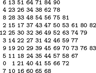
This table gives the output that is produced when Program 4.19 is invoked with 84 as the command-line argument. The 10 queues have an average of 8.4 items each, ranging from a low of six to a high of 11.
Figure 4.13 Random-queue simulation
Program 4.20 is an implementation of the FIFO queue ADT defined in Program 4.18, using linked lists for the underlying data structure. The primary difference between these implementations and those in Program 4.10 has to do with the variables head and tail.
In Program 4.10, we had only one queue, so we simply declared and used these variables in the implementation. In Program 4.20, each queue q has its own pointers head and tail, which we reference with the code q->head and q->tail. The definition of struct queue in an implementation answers the question “what is a queue?” for that implementation: In this case, the answer is that a queue is pointer to a structure consisting of the links to the head and tail of the queue. In an array implementation, a queue is a pointer to a struct consisting of a pointer to an array and two integers: the size of the array and the number of elements currently on the queue (see Exercise 4.65). In general, the members of the structure are exactly the global or static variables from the one-object implementation.
With a carefully designed ADT, we can make use of the separation between client and implementations in many interesting ways. For example, we commonly use driver programs when developing or debugging ADT implementations. Similarly, we often use incomplete implementations of ADTs, called stubs, as placeholders while building systems to learn properties of clients, although this exercise can be tricky for clients that depend on the ADT implementation semantics.
As we saw in Section 4.3, the ability to have multiple instances of a given ADT in a single program can lead us to complicated situations. Do we want to be able to have stacks or queues with different types of objects on them? How about different types of objects on the same queue? Do we want to use different implementations for queues of the same type in a single client because we know of performance differences? Should information about the efficiency of implementations be included in the interface? What form should that information take? Such questions underscore the importance of understanding the basic characteristics of our algorithms and data structures and how client programs may use them effectively, which is, in a sense, the topic of this book. Full implementations, however, are exercises in software engineering, rather than in algorithms design, so we stop short of developing ADTs of such generality in this book (see reference section).
Despite its virtues, our mechanism for providing first-class ADTs comes at the (slight) cost of extra pointer dereferences and slightly more complicated implementation code, so we shall use the full mechanism for only those ADTs that require the use of handles as arguments or return values in interfaces. On the one hand, the use of first-class types might encompass the majority of the code in a small number of huge applications systems; on the other hand, an only-one-object arrangement—such as the stacks, FIFO queues, and generalized queues of Sections 4.2 through 4.7—and the use of typedef to specify the types of objects as described in Section 4.1 are quite serviceable techniques for many of the programs that we write. In this book, we introduce most of the algorithms and data structures that we consider in the latter context, then extend these implementations into first-class ADTs when warranted.
Exercises
![]() 4.57 Add a function
4.57 Add a function COMPLEXadd to the ADT for complex numbers in the text (Programs 4.16 and 4.17).
4.58 Convert the equivalence-relations ADT in Section 4.5 to a first-class type.
4.59 Create a first-class ADT for use in programs that process playing cards.
![]() 4.60 Write a program to determine empirically the probability that various poker hands are dealt, using your ADT from Exercise 4.59.
4.60 Write a program to determine empirically the probability that various poker hands are dealt, using your ADT from Exercise 4.59.
4.61 Create an ADT for points in the plane, and change the closest-point program in Chapter 3 Program 3.16 to a client program that uses your ADT.
![]() 4.62 Develop an implementation for the complex-number ADT that is based on representing complex numbers in polar coordinates (that is, in the form reiθ).
4.62 Develop an implementation for the complex-number ADT that is based on representing complex numbers in polar coordinates (that is, in the form reiθ).
![]() 4.63 Use the identity eiθ = cos θ + i sin θ to prove that e2πi = 1 and that the N complex Nth roots of unity are
4.63 Use the identity eiθ = cos θ + i sin θ to prove that e2πi = 1 and that the N complex Nth roots of unity are
for k = 0, 1, ..., N – 1.
4.64 List the Nth roots of unity for N from 2 through 8.
4.65 Develop an implementation of the FIFO queue first-class ADT given in the text (Program 4.18) that uses an array as the underlying data structure.
![]() 4.66 Write an interface for a first-class pushdown-stack ADT.
4.66 Write an interface for a first-class pushdown-stack ADT.
4.67 Develop an implementation of your first-class pushdown-stack ADT from Exercise 4.66 that uses an array as the underlying data structure.
4.68 Develop an implementation of your first-class pushdown-stack ADT from Exercise 4.66 that uses a linked list as the underlying data structure.
![]() 4.69 Modify the postfix-evaluation program in Section 4.3 to evaluate post-fix expressions consisting of complex numbers with integer coefficients, using the first-class complex numbers ADT in the text (Programs 4.16 and 4.17). For simplicity, assume that the complex numbers all have nonnull integer coefficients for both real and imaginary parts and are written with no spaces. For example, your program should print the output
4.69 Modify the postfix-evaluation program in Section 4.3 to evaluate post-fix expressions consisting of complex numbers with integer coefficients, using the first-class complex numbers ADT in the text (Programs 4.16 and 4.17). For simplicity, assume that the complex numbers all have nonnull integer coefficients for both real and imaginary parts and are written with no spaces. For example, your program should print the output 8+4i when given the input
1+1i 0+1i + 1-2i * 3+4i + .
4.9 Application-Based ADT Example
As a final example, we consider in this section an application-specific ADT that is representative of the relationship between applications domains and the algorithms and data structures of the type that we consider in this book. The example that we shall consider is the polynomial ADT. It is drawn from symbolic mathematics, where we use the computer to help us manipulate abstract mathematical objects.
Our goal is to be able to perform computations such as
We also want to be able to evaluate the polynomial for a given value of x. For x = 0.5, both sides of this equation have the value 1.1328125. The operations of multiplying, adding, and evaluating polynomials are at the heart of a great many mathematical calculations. Program 4.21 is a simple example that performs the symbolic operations corresponding to the polynomial equations
The same basic ideas extend to include operations such as composition, integration, differentiation, knowledge of special functions, and so forth.
The first step is to define the polynomial ADT, as illustrated in the interface Program 4.22. For a well-understood mathematical abstraction such as a polynomial, the specification is so clear as to be unspoken (in the same way as for the ADT for complex numbers that we discussed in Section 4.8): We want instances of the ADT to behave precisely in the same manner as the well-understood mathematical abstraction.
To implement the functions defined in the interface, we need to choose a particular data structure to represent polynomials and then to implement algorithms that manipulate the data structure to produce the behavior that client programs expect from the ADT. As usual, the choice of data structure affects the potential efficiency of the algorithms, and we are free to consider several. Also as usual, we have the choice of using a linked representation or an array representation. Program 4.23 is an implementation using an array representation; the linked-list representation is left as an exercise (see Exercise 4.70).
To add two polynomials, we add their coefficients. If the polynomials are represented as arrays, the add function amounts to a single loop through the arrays, as shown in Program 4.23. To multiply two polynomials, we use the elementary algorithm based on the distributive law. We multiply one polynomial by each term in the other, line up the results so that powers of x match, then add the terms to get the final result. The following table summarizes the computation for (1 – x + x2/2 – x3/6)(1 + x + x2 + x3):
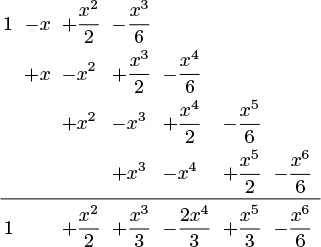
The computation seems to require time proportional to N2 to multiply two polynomials. Finding a faster algorithm for this task is a significant challenge. We shall consider this topic in detail in Part 8, where we shall see that it is possible to accomplish the task in time proportional to N3/2 using a divide-and-conquer algorithm, and in time proportional to N lg N using the fast Fourier transform.
The implementation of the evaluate function in Program 4.23 uses a classic efficient algorithm known as Horner’s algorithm. A naive implementation of the function involves a direct computation using a function that computes xN. This approach takes quadratic time. A less naive implementation involves saving the values of xi in a table, then using them in a direct computation. This approach takes linear extra space. Horner’s algorithm is a direct optimal linear algorithm based on parenthesizations such as
a4x4 + a3x3 + a2x2 + a1x + a0 = (((a4x + a3)x + a2)x + a1)x + a0.
Horner’s method is often presented as a time-saving trick, but it is actually an early and outstanding example of an elegant and efficient algorithm, which reduces the time required for this essential computational task from quadratic to linear. The calculation that we performed in Program 4.2 for converting ASCII strings to integers is a version of Horner’s algorithm. We shall encounter Horner’s algorithm again, in Chapter 14 and Part 5, as the basis for an important computation related to certain symbol-table and string-search implementations.
For simplicity and efficiency, POLYadd modifies one of its arguments; if we choose to use this implementation in an application, we should note that fact in the specification (see Exercise 4.71). Moreover, we have memory leaks, particularly in POLYmult, which creates a new polynomial to hold the result (see Exercise 4.72).
As usual, the array representation for implementing the polynomial ADT is but one possibility. If exponents are huge and there are not many terms, a linked-list representation might be more appropriate. For example, we would not want to use Program 4.23 to perform a multiplication such as
(1 + x1000000)(1 + x2000000) = 1 + x1000000 + x2000000 + x3000000,
because it would use an array with space for hundreds of thousands of unused coefficients. Exercise 4.70 explores the linked list option in more detail.
Exercises
4.70 Provide an implementation for the polynomial ADT given in the text (Program 4.22) that uses linked lists as the underlying data structure. Your lists should not contain any nodes corresponding to terms with coefficient value 0.
![]() 4.71 Modify the implementation of
4.71 Modify the implementation of POLYadd in Program 4.23 such that it operates in a manner similar to POLYmult (and does not modify either of its arguments).
![]() 4.72 Modify the polynomial ADT interface, implementation, and client in the text (Programs 4.21 through 4.23) such that there are no memory leaks. To do so, define new operations
4.72 Modify the polynomial ADT interface, implementation, and client in the text (Programs 4.21 through 4.23) such that there are no memory leaks. To do so, define new operations POLYdestroy and POLYcopy, which should free the memory for an object and copy one object’s values to another, respectively; and modify POLYadd and POLYmult to destroy their arguments and return a newly created object, by convention.
![]() 4.73 Extend the polynomial ADT given in the text to include integration and differentiation of polynomials.
4.73 Extend the polynomial ADT given in the text to include integration and differentiation of polynomials.
![]() 4.74 Modify your polynomial ADT from Exercise 4.73 to ignore all terms with exponents greater than or equal to an integer M, which is provided by the client at initialization.
4.74 Modify your polynomial ADT from Exercise 4.73 to ignore all terms with exponents greater than or equal to an integer M, which is provided by the client at initialization.
![]() 4.75 Extend your polynomial ADT from Exercise 4.73 to include polynomial division and composition.
4.75 Extend your polynomial ADT from Exercise 4.73 to include polynomial division and composition.
![]() 4.76 Develop an ADT that allows clients to perform addition and multiplication of arbitrarily long integers.
4.76 Develop an ADT that allows clients to perform addition and multiplication of arbitrarily long integers.
![]() 4.77 Modify the postfix-evaluation program in Section 4.3 to evaluate post-fix expressions consisting of arbitrarily long integers, using the ADT that you developed for Exercise 4.76.
4.77 Modify the postfix-evaluation program in Section 4.3 to evaluate post-fix expressions consisting of arbitrarily long integers, using the ADT that you developed for Exercise 4.76.
![]() 4.78 Write a client program that uses your polynomial ADT from Exercise 4.75 to evaluate integrals by using Taylor series approximations of functions, manipulating them symbolically.
4.78 Write a client program that uses your polynomial ADT from Exercise 4.75 to evaluate integrals by using Taylor series approximations of functions, manipulating them symbolically.
4.79 Develop an ADT that provides clients with the ability to perform algebraic operations on vectors of floating-point numbers.
4.80 Develop an ADT that provides clients with the ability to perform algebraic operations on matrices of abstract objects for which addition, subtraction, multiplication, and division are defined.
4.81 Write an interface for a character-string ADT, which includes operations for creating a string, comparing two strings, concatenating two strings, copying one string to another, and returning the string length.
4.82 Provide an implementation for your string ADT interface from Exercise 4.81, using the C string library where appropriate.
4.83 Provide an implementation for your string ADT interface from Exercise 4.81, using a linked list for the underlying representation. Analyze the worst-case running time of each operation.
4.84 Write an interface and an implementation for an index set ADT, which processes sets of integers in the range 0 to M – 1 (where M is a defined constant) and includes operations for creating a set, computing the union of two sets, computing the intersection of two sets, computing the complement of a set, computing the difference of two sets, and printing out the contents of a set. In your implementation, use an array of M – 1 0-1 values to represent each set.
4.85 Write a client program that tests your ADT from Exercise 4.84.
4.10 Perspective
There are three primary reasons for us to be aware of the fundamental concepts underlying ADTs as we embark on the study of algorithms and data structures:
• ADTs are an important software-engineering tool in widespread use, and many of the algorithms that we study serve as implementations for fundamental ADTs that are widely applicable.
• ADTs help us to encapsulate the algorithms that we develop, so that we can use the same code for many different purposes.
• ADTs provide a convenient mechanism for our use in the process of developing and comparing the performance of algorithms.
Ideally, ADTs embody the common-sense principle that we are obligated to describe precisely the ways in which we manipulate our data. The client-interface-implementation mechanism that we have considered in detail in this chapter is convenient for this task in C, and provides us with C code that has a number of desirable properties. Many modern languages have specific support that allows the development of programs with similar properties, but the general approach transcends particular languages—when we do not have specific language support, we adopt programming conventions to maintain the separation that we would like to have among clients, interfaces, and implementations.
As we consider an ever-expanding set of choices in specifying the behavior of our ADTs, we are faced with an ever-expanding set of challenges in providing efficient implementations. The numerous examples that we have considered illustrate ways of meeting such challenges. We continually strive to achieve the goal of implementing all the operations efficiently, but we are unlikely to have a general-purpose implementation that can do so for all sets of operations. This situation works against the principles that lead us to ADTs in the first place, because in many cases implementors of ADTs need to know properties of client programs to know which implementations of associated ADTs will perform most efficiently, and implementors of client programs need to know performance properties of various implementations to know which to choose for a particular application. As ever, we must strike a balance. In this book, we consider numerous approaches to implementations for variants of fundamental ADTs, all of which have important applications.
We can use one ADT to build another. We have used the pointer and structure abstractions provided by C to build linked lists, then we have used linked lists or the array abstraction provided by C to build pushdown stacks, then we use pushdown stacks to get the capability to evaluate arithmetic expressions. The ADT concept allows us to construct large systems on different layers of abstraction, from the machine-language instructions provided by the computer, to the various capabilities provided by the programming language, to sorting, searching and other higher-level capabilities provided by algorithms as discussed in Parts 3 and 4 of this book, to the even higher levels of abstraction that the various applications require, as discussed in Parts 5 through 8. ADTs are one point on the continuum of developing ever more powerful abstract mechanisms that is the essence of using computers effectively in problem solving.