Chapter Ten. Radix Sorting
For many sorting applications, the keys used to define the order of the records for files can be complicated. For example, consider the complex nature of the keys used in a telephone book or a library catalog. To separate this complication from essential properties of the sorting methods that we have been studying, we have used just the basic operations of comparing two keys and exchanging two records (hiding all the details of manipulating keys in these functions) as the abstract interface between sorting methods and applications for most of the methods in Chapters 6 through 9. In this chapter, we examine a different abstraction for sort keys. For example, processing the full key at every step is often unnecessary: to look up a person’s number in a telephone book, we often just check the first few letters in the name to find the page containing the number. To gain similar efficiencies in sorting algorithms, we shall shift from the abstract operation where we compare keys to an abstraction where we decompose keys into a sequence of fixed-sized pieces, or bytes. Binary numbers are sequences of bits, strings are sequences of characters, decimal numbers are sequences of digits, and many other (but not all) types of keys can be viewed in this way. Sorting methods built on processing numbers one piece at a time are called radix sorts. These methods do not just compare keys: They process and compare pieces of keys.
Radix-sorting algorithms treat the keys as numbers represented in abase-R number system, for various values of R (the radix), and work with individual digits of the numbers. For example, when a machine at the post office processes a pile of packages that have on them five-digit decimal numbers, it distributes the packages into ten piles: one having numbers beginning with 0, one having numbers beginning with 1, one having numbers beginning with 2, and so forth. If necessary, the piles can be processed individually, by using the same method on the next digit or by using some easier method if there are only a few packages. If we were to pick up the packages in the piles in order from 0 to 9 and in order within each pile after they have been processed, we would get them in sorted order. This procedure is a simple example of a radix sort with R = 10, and it is the method of choice in many real sorting applications where keys are 5- to 10-digit decimal numbers, such as postal codes, telephone numbers or social-security numbers. We shall examine the method in detail in Section 10.3.
Different values of the radix R are appropriate in various applications. In this chapter, we focus primarily on keys that are integers or strings, where radix sorts are widely used. For integers, because they are represented as binary numbers in computers, we most often work with R = 2 or some power of 2, because this choice allows us to decompose keys into independent pieces. For keys that involve strings of characters, we use R = 128 or R = 256, aligning the radix with the byte size. Beyond such direct applications, we can ultimately treat virtually anything that is represented inside a digital computer as a binary number, and we can recast many sorting applications using other types of keys to make feasible the use of radix sorts operating on keys that are binary numbers.
Radix-sorting algorithms are based on the abstract operation “extract the ith digit from a key.” Fortunately, C provides low-level operators that make it possible to implement such an operation in a straightforward and efficient manner. This fact is significant because many other languages (for example, Pascal), to encourage us to write machine-independent programs, intentionally make it difficult to write a program that depends on the way that a particular machine represents numbers. In such languages, it is difficult to implement many types of bit-by-bit manipulation techniques that actually suit most computers well. Radix sorting in particular was, for a time, a casualty of this “progressive” philosophy. But the designer of C recognized that direct manipulation of bits is often useful, and we shall be able to take advantage of C’s low-level facilities to implement radix sorts.
Good hardware support also is required; and it cannot be taken for granted. Some machines (both old and new) provide efficient ways to get at small data, but some other machines (both old and new) slow down significantly when such operations are used. Whereas radix sorts are simply expressed in terms of the extract-the-digit operation, the task of getting peak performance out of a radix sorting algorithm can be a fascinating introduction to our hardware and software environment.
There are two, fundamentally different, basic approaches to radix sorting. The first class of methods involves algorithms that examine the digits in the keys in a left-to-right order, working with the most significant digits first. These methods are generally referred to as most-significant-digit (MSD) radix sorts. MSD radix sorts are attractive because they examine the minimum amount of information necessary to get a sorting job done (see Figure 10.1). MSD radix sorts generalize quicksort, because they work by partitioning the file to be sorted according to the leading digits of the keys, then recursively applying the same method to the subfiles. Indeed, when the radix is 2, we implement MSD radix sorting in a manner similar to that for quicksort. The second class of radix-sorting methods is different: They examine the digits in the keys in a right-to-left order, working with the least significant digits first. These methods are generally referred to as least-significant-digit (LSD) radix sorts. LSD radix sorts are somewhat counterintuitive, since they spend processing time on digits that cannot affect the result, but it is easy to ameliorate this problem, and this venerable approach is the method of choice for many sorting applications.
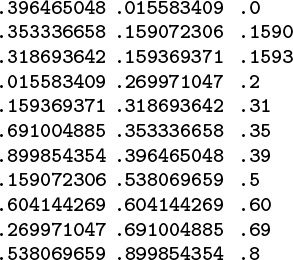
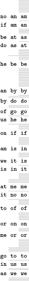
Even though the 11 numbers between 0 and 1 on this list (left) each have nine digits for a total of 99 digits, we can put them in order (center) by just examining 22 of the digits (right).
Figure 10.1 MSD radix sorting
10.1 Bits, Bytes, and Words
The key to understanding radix sort is to recognize that (i) computers generally are built to process bits in groups called machine words, which are often grouped into smaller pieces call bytes; (ii) sort keys also are commonly organized as byte sequences; and (iii) small byte sequences can also serve as array indices or machine addresses. Therefore, it will be convenient for us to work with the following abstractions.
Definition 10.1 A byte is a fixed-length sequence of bits; a string is a variable-length sequence of bytes; a word is a fixed-length sequence of bytes.
In radix sorting, depending on the context, a key may be a word or a string. Some of the radix-sorting algorithms that we consider in this chapter depend on the keys being fixed length (words); others are designed to adapt to the situation when the keys are variable length (strings).
A typical machine might have 8-bit bytes and 32- or 64-bit words (the actual values may be found in the header file <limits.h>), but it will be convenient for us to consider various other byte and word sizes as well (generally small integer multiples or fractions of built-in machine sizes). We use machine- and application-dependent defined constants for the number of bits per word and the number of bits per byte:
#define bitsword 32
#define bitsbyte 8
#define bytesword 4
#define R (1 << bitsbyte)
Also included in these definitions for use when we begin looking at radix sorts is the constant R, the number of different byte values. When using these definitions, we generally assume that bitsword is a multiple of bitsbyte; that the number of bits per machine word is not less than (typically, is equal to) bitsword; and that bytes are individually addressable. Different computers have different conventions for referring to their bits and bytes; for the purposes of our discussion, we will consider the bits in a word to be numbered, left to right, from 0 to bitsword-1, and the bytes in a word to be numbered, left to right, from 0 to bytesword-1. In both cases, we assume the numbering to also be from most significant to least significant.
Most computers have bitwise and and shift operations, which we can use to extract bytes from words. In C, we can directly express the operation of extracting the Bth byte of a binary word A as follows:
#define digit(A, B)
(((A) >> (bitsword-((B)+1)*bitsbyte)) & (R-1))
For example, this macro would extract byte 2 (the third byte) of a 32-bit number by shifting right 32 – 3 * 8 = 8 bit positions, then using the mask 00000000000000000000000011111111 to zero out all the bits except those of the desired byte, in the 8 bits at the right.
Another option on many machines is to arrange things such that the radix is aligned with the byte size, and therefore a single access will get the right bits quickly. This operation is supported directly for strings in C:
#define digit(A, B) A[B].
This approach could be used for numbers as well, though differing number-representation schemes may make such code nonportable. In any case, we need to be aware that byte-access operations of this type might be implemented with underlying shift-and-mask operations similar to the ones in the previous paragraph in some computing environments.
At a slightly different level of abstraction, we can think of keys as numbers and bytes as digits. Given a (key represented as a) number, the fundamental operation needed for radix sorts is to extract a digit from the number. When we choose a radix that is a power of 2, the digits are groups of bits, which we can easily access directly using one of the macros just discussed. Indeed, the primary reason that we use radices that are powers of 2 is that the operation of accessing groups of bits is inexpensive. In some computing environments, we can use other radices, as well. For example, if a is a positive integer, the bth digit (from the right) of the radix-R representation of a is
![]() a/Rb
a/Rb![]() mod R.
mod R.
On a machine built for high-performance numerical calculations, this computation might be as fast for general R as for R =2.
Yet another viewpoint is to think of keys as numbers between 0 and 1 with an implicit decimal point at the left, as shown in Figure 10.1. In this case, the bth digit (from the left) of a is
![]() aRb
aRb![]() mod R.
mod R.
If we are using a machine where we can do such operations efficiently, then we can use them as the basis for our radix sort. This model applies when keys are variable length, such as character strings.
Thus, for the remainder of this chapter, we view keys as radix-R numbers (with R not specified), and use the abstract digit operation to access digits of keys, with confidence that we will be able to develop fast implementations of digit for particular computers.
Definition 10.2 A key is a radix-R number, with digits numbered from the left (starting at 0).
In light of the examples that we just considered, it is safe for us to assume that this abstraction will admit efficient implementations for many applications on most computers, although we must be careful that a particular implementation is efficient within a given hardware and software environment.
We assume that the keys are not short, so it is worthwhile to extract their bits. If the keys are short, then we can use the key-indexed counting method of Chapter 6. Recall that this method can sort N keys known to be integers between 0 and R – 1 in linear time, using one auxiliary table of size R for counts and another of size N for rearranging records. Thus, if we can afford a table of size 2w, then w-bit keys can easily be sorted in linear time. Indeed, key-indexed counting lies at the heart of the basic MSD and LSD radix-sorting methods. Radix sorting comes into play when the keys are sufficiently long (say w = 64) that using a table of size 2w is not feasible.
Exercises
![]() 10.1 How many digits are there when a 32-bit quantity is viewed as a radix-256 number? Describe how to extract each of the digits. Answer the same question for radix 216.
10.1 How many digits are there when a 32-bit quantity is viewed as a radix-256 number? Describe how to extract each of the digits. Answer the same question for radix 216.
![]() 10.2 For N = 103, 106, and 109, give the smallest byte size that allows any number between 0 and N to be represented in a 4-byte word.
10.2 For N = 103, 106, and 109, give the smallest byte size that allows any number between 0 and N to be represented in a 4-byte word.
![]() 10.3 Implement a
10.3 Implement a less function using the digit abstraction (so that, for example, we could run empirical studies comparing the algorithms in Chapters 6 and 9 with the methods in this chapter, using the same data).
![]() 10.4 Design and carry out an experiment to compare the cost of extracting digits using bit-shifting and arithmetic operations on your machine. How many digits can you extract per second, using each of the two methods? Note: Be wary; your compiler might convert arithmetic operations to bit-shifting ones, or vice versa!
10.4 Design and carry out an experiment to compare the cost of extracting digits using bit-shifting and arithmetic operations on your machine. How many digits can you extract per second, using each of the two methods? Note: Be wary; your compiler might convert arithmetic operations to bit-shifting ones, or vice versa!
![]() 10.5 Write a program that, given a set of N random decimal numbers (R = 10) uniformly distributed between 0 and 1, will compute the number of digit comparisons necessary to sort them, in the sense illustrated in Figure 10.1. Run your program for N = 103, 104, 105, and 106.
10.5 Write a program that, given a set of N random decimal numbers (R = 10) uniformly distributed between 0 and 1, will compute the number of digit comparisons necessary to sort them, in the sense illustrated in Figure 10.1. Run your program for N = 103, 104, 105, and 106.
![]() 10.6 Answer Exercise 10.5 for R = 2, using random 32-bit quantities.
10.6 Answer Exercise 10.5 for R = 2, using random 32-bit quantities.
![]() 10.7 Answer Exercise 10.5 for the case where the numbers are distributed according to a Gaussian distribution.
10.7 Answer Exercise 10.5 for the case where the numbers are distributed according to a Gaussian distribution.
10.2 Binary Quicksort
Suppose that we can rearrange the records of a file such that all those whose keys begin with a 0 bit come before all those whose keys begin with a 1 bit. Then, we can use a recursive sorting method that is a variant of quicksort (see Chapter 7): Partition the file in this way, then sort the two subfiles independently. To rearrange the file, scan from the left to find a key that starts with a 1 bit, scan from the right to find a key that starts with a 0 bit, exchange, and continue until the scanning pointers cross. This method is often called radix-exchange sort in the literature (including in earlier editions of this book); here, we shall use the name binary quicksort to emphasize that it is a simple variant of the algorithm invented by Hoare, even though it was actually discovered before quicksort was (see reference section).
Program 10.1 is a full implementation of this method. The partitioning process is essentially the same as Program 7.2, except that the number 2b, instead of some key from the file, is used as the partitioning element. Because 2b may not be in the file, there can be no guarantee that an element is put into its final place during partitioning. The algorithm also differs from normal quicksort because the recursive calls are for keys with 1 fewer bit. This difference has important implications for performance. For example, when a degenerate partition occurs for a file of N elements, a recursive call for a subfile of size N will result, for keys with 1 fewer bit. Thus, the number of such calls is limited by the number of bits in the keys. By contrast, consistent use of partitioning values not in the file in a standard quicksort could result in an infinite recursive loop.
As there are with standard quicksort, various options are available in implementing the inner loop. In Program 10.1, tests for whether the pointers have crossed are included in both inner loops. This arrangement results in an extra exchange for the case i = j, which could be avoided with a break, as is done in Program 7.2, although in this case the exchange of a[i] with itself is harmless. Another alternative is to use sentinel keys.
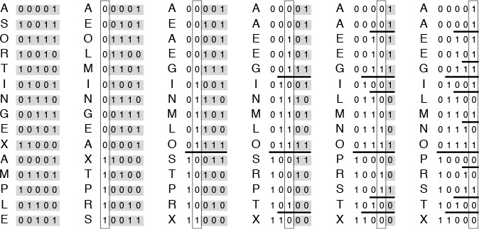
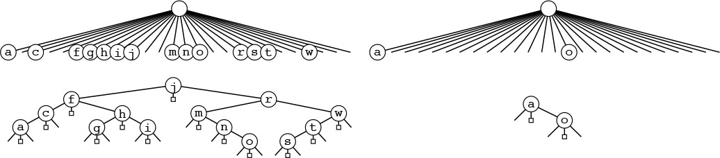
Figure 10.2 depicts the operation of Program 10.1 on a small sample file, for comparison with Figure 7.1 for quicksort. This figure shows what the data movement is, but not why the various moves are made—that depends on the binary representation of the keys. A more detailed view for the same example is given in Figure 10.3. This example assumes that the letters are encoded with a simple 5-bit code, with the ith letter of the alphabet represented by the binary representation of the number i. This encoding is a simplified version of real character codes, which use more bits (7, 8, or even 16) to represent more characters (uppercase or lowercase letters, numbers, and special symbols).
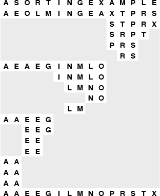
Partitioning on the leading bit does not guarantee that one value will be put into place; it guarantees only that all keys with leading 0 bits come before all keys with leading 1 bits. We can compare this diagram with Figure 7.1 for quicksort, although the operation of the partitioning method is completely opaque without the binary representation of the keys. Figure 10.3 gives the details that explain the partition positions precisely.
Figure 10.2 Binary quicksort example
We derive this figure from Figure 10.2 by translating the keys to their binary encoding, compressing the table such that the independent subfile sorts are shown as though they happen in parallel, and transposing rows and columns. The first stage splits the file into a subfile with all keys beginning with 0, and a subfile with all keys beginning with 1. Then, the first subfile is split into one subfile with all keys beginning with 00, and another with all keys beginning with 01; independently, at some other time, the other subfile is split into one subfile with all keys beginning with 10, and another with all keys beginning with 11. The process stops when the bits are exhausted (for duplicate keys, in this example) or the subfiles are of size 1.
Figure 10.3 Binary quicksort example (key bits exposed)
For full-word keys consisting of random bits, the starting point in Program 10.1 should be the leftmost bit of the words, or bit 0. In general, the starting point that should be used depends in a straightforward way on the application, on the number of bits per word in the machine, and on the machine representation of integers and negative numbers. For the one-letter 5-bit keys in Figures 10.2 and 10.3, the starting point on a 32-bit machine would be bit 27.
This example highlights a potential problem with binary quicksort in practical situations: Degenerate partitions (partitions with all keys having the same value for the bit being used) can happen frequently. It is not uncommon to sort small numbers (with many leading zeros) as in our examples. The problem also occurs in keys comprising characters: for example, suppose that we make up 32-bit keys from four characters by encoding each in a standard 8-bit code and then putting them together. Then, degenerate partitions are likely to occur at the beginning of each character position, because, for example, lowercase letters all begin with the same bits in most character codes. This problem is typical of the effects that we need to address when sorting encoded data, and similar problems arise in other radix sorts.
Once a key is distinguished from all the other keys by its left bits, no further bits are examined. This property is a distinct advantage in some situations; it is a disadvantage in others. When the keys are truly random bits, only about lg N bits per key are examined, and that could be many fewer than the number of bits in the keys. This fact is discussed in Section 10.6; see also Exercise 10.5 and Figure 10.1. For example, sorting a file of 1000 records with random keys might involve examining only about 10 or 11 bits from each key (even if the keys are, say, 64-bit keys). On the other hand, all the bits of equal keys are examined. Radix sorting simply does not work well on files that contain huge numbers of duplicate keys that are not short. Binary quicksort and the standard method are both fast if keys to be sorted comprise truly random bits (the difference between them is primarily determined by the difference in cost between the bit-extraction and comparison operations), but the standard quicksort algorithm can adapt better to nonrandom sets of keys, and 3-way quicksort is ideal when duplicate keys predominate.
As it was with quicksort, it is convenient to describe the partitioning structure with a binary tree (as depicted in Figure 10.4): The root corresponds to a subfile to be sorted, and its two subtrees correspond to the two subfiles after partitioning. In standard quicksort, we know that at least one record is put into position by the partitioning process, so we put that key into the root node; in binary quicksort, we know that keys are in position only when we get to a subfile of size 1 or we have exhausted the bits in the keys, so we put the keys at the bottom of the tree. Such a structure is called a binary trie—properties of tries are covered in detail in Chapter 15. For example, one important property of interest is that the structure of the trie is completely determined by the key values, rather than by their order.
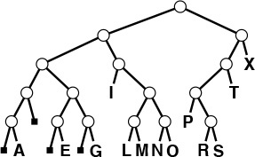
This tree describes the partitioning structure for binary quicksort, corresponding to Figures 10.2 and 10.3. Because no item is necessarily put into position, the keys correspond to external nodes in the tree. The structure has the following property: Following the path from the root to any key, taking 0 for left branches and 1 for right branches, gives the leading bits of the key. These are precisely the bits that distinguish the key from other keys during the sort. The small black squares represent the null partitions (when all the keys go to the other side because their leading bits are the same). This happens only near the bottom of the tree in this example, but could happen higher up in the tree: For example, if I or X were not among the keys, their node would be replaced by a null node in this drawing. Note that duplicated keys (A and E) cannot be partitioned (the sort puts them in the same subfile only after all their bits are exhausted).
Figure 10.4 Binary quicksort partitioning trie
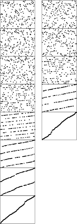
Partitioning divisions in binary quicksort depend on the binary representation of the range and number of items being sorted. For example, if the files are random permutations of the integers less than 171 = 101010112, then partitioning on the first bit is equivalent to partitioning about the value 128, so the subfiles are unequal (one of size 128 and the other of size 43). The keys in Figure 10.5 are random 8-bit values, so this effect is absent there, but the effect is worthy of note now, lest it come as a surprise when we encounter it in practice.
Partitioning divisions in binary quicksort are less sensitive to key order than they are in standard quicksort. Here, two different random 8-bit files lead to virtually identical partitioning profiles.
Figure 10.5 Dynamic characteristics of binary quicksort on a large file
We can improve the basic recursive implementation in Program 10.1 by removing recursion and treating small subfiles differently, just as we did for standard quicksort in Chapter 7.
Exercises
![]() 10.8 Draw the trie in the style of Figure 10.2 that corresponds to the partitioning process in radix quicksort for the key E A S Y Q U E S T I O N.
10.8 Draw the trie in the style of Figure 10.2 that corresponds to the partitioning process in radix quicksort for the key E A S Y Q U E S T I O N.
10.9 Compare the number of exchanges used by binary quicksort with the number used by the normal quicksort for the file of 3-bit binary numbers 001, 011, 101, 110, 000, 001, 010, 111, 110, 010.
![]() 10.10 Why is it not as important to sort the smaller of the two subfiles first in binary quicksort as it was for normal quicksort?
10.10 Why is it not as important to sort the smaller of the two subfiles first in binary quicksort as it was for normal quicksort?
![]() 10.11 Describe what happens on the second level of partitioning (when the left subfile is partitioned and when the right subfile is partitioned) when we use binary quicksort to sort a random permutation of the nonnegative integers less than 171.
10.11 Describe what happens on the second level of partitioning (when the left subfile is partitioned and when the right subfile is partitioned) when we use binary quicksort to sort a random permutation of the nonnegative integers less than 171.
10.12 Write a program that, in one preprocessing pass, identifies the number of leading bit positions where all keys are equal, then calls a binary quicksort that is modified to ignore those bit positions. Compare the running time of your program with that of the standard implementation for N = 103, 104, 105, and 106 when the input is 32-bit words of the following format: The rightmost 16 bits are uniformly random, and the leftmost 16 bits are all 0 except with a 1 in position i if there are i 1s in the right half.
10.13 Modify binary quicksort to check explicitly for the case that all keys are equal. Compare the running time of your program with that of the standard implementation for N = 103, 104, 105, and 106 with the input described in Exercise 10.12.
10.3 MSD Radix Sort
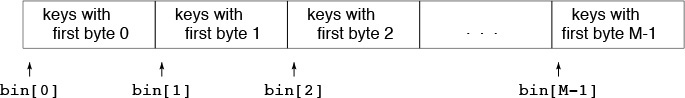
Using just 1 bit in radix quicksort amounts to treating keys as radix-2 (binary) numbers and considering the most significant digits first. Generalizing, suppose that we wish to sort radix-R numbers by considering the most significant bytes first. Doing so requires partitioning the array into R, rather than just two, different parts. Traditionally we refer to the partitions as bins or buckets and think of the algorithm as using a group of R bins, one for each possible value of the first digit, as indicated in the following diagram:
We pass through the keys, distributing them among the bins, then recursively sort the bin contents on keys with 1 fewer byte.
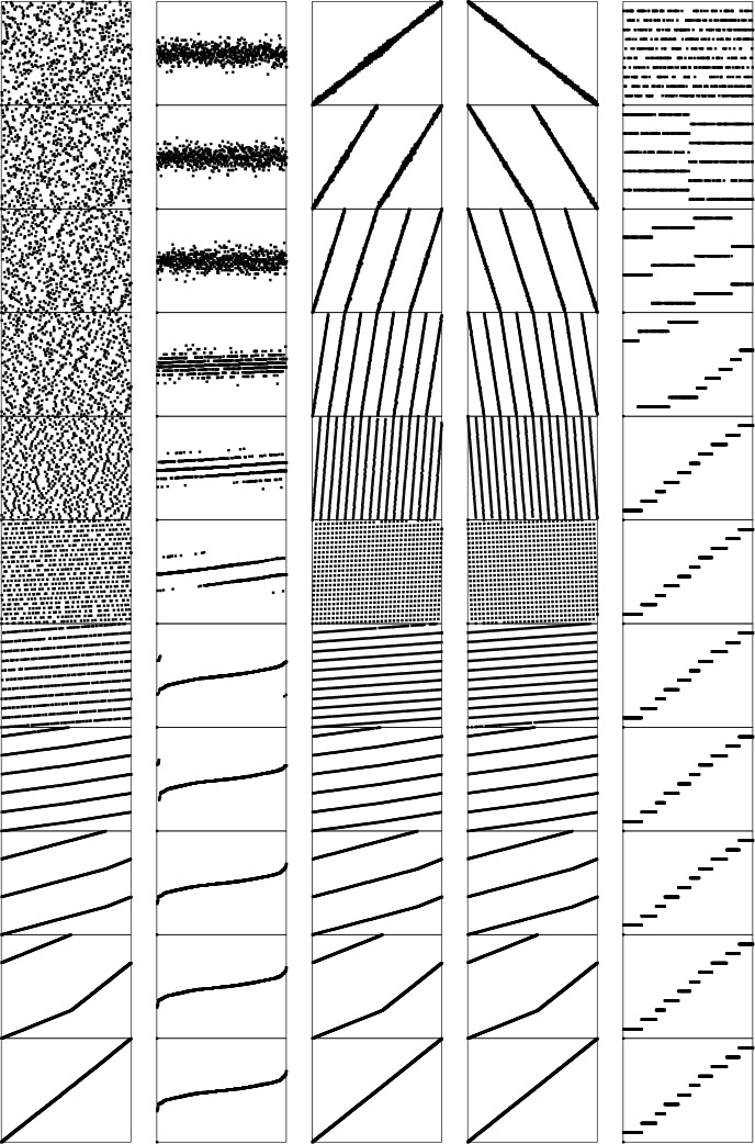
Figure 10.6 shows an example of MSD radix sorting on a random permutation of integers. By contrast with binary quicksort, this algorithm can bring a file nearly into order rather quickly, even on the first partition, if the radix is sufficiently large.

Just one stage of MSD radix sort can nearly complete a sort task, as shown in this example with random 8-bit integers. The first stage of an MSD sort, on the leading 2 bits (left), divides the file into four subfiles. The next stage divides each of those into four subfiles. An MSD sort on the leading 3 bits (right) divides the file into eight subfiles, in just one distribution-counting pass. At the next level, each of those subfiles is divided into eight parts, leaving just a few elements in each.
Figure 10.6 Dynamic characteristics of MSD radix sort
As mentioned in Section 10.2, one of the most attractive features of radix sorting is the intuitive and direct manner in which it adapts to sorting applications where keys are strings of characters. This observation is especially true in C and other programming environments that provide direct support for processing strings. For MSD radix sorting, we simply use a radix corresponding to the byte size. To extract a digit, we load a byte; to move to the next digit, we increment a string pointer. For the moment, we consider fixed-length keys; we shall see shortly that variable-length string keys are easy to handle with the same basic mechanisms.
Figure 10.7 shows an example of MSD radix sorting on three-letter words. For simplicity, this figure assumes that the radix is 26, although in most applications we would use a larger radix corresponding to the character encodings. First, the words are partitioned so all those that start with a appear before those that start with b, and so forth. Then, the words that start with a are sorted recursively, then the words that start with b are sorted, and so forth. As is obvious from the example, most of the work in the sort lies in partitioning on the first letter; the subfiles that result from the first partition are small.
We divide the words into 26 bins according to the first letter. Then, we sort all the bins by the same method, starting at the second letter.
Figure 10.7 MSD radix sort example
As we saw for quicksort in Chapter 7 and Section 10.2 and for mergesort in Chapter 8, we can improve the performance of most recursive programs by using a simple algorithm for small cases. Using a different method for small subfiles (bins containing a small number of elements) is essential for radix sorting, because there are so many of them! Moreover, we can tune the algorithm by adjusting the value of R because there is a clear tradeoff: If R is too large, the cost of initializing and checking the bins dominates; if it is too small, the method does not take advantage of the potential gain available by subdividing into as many pieces as possible. We return to these issues at the end of this section and in Section 10.6.
To implement MSD radix sort, we need to generalize the methods for partitioning an array that we studied in relation to quicksort implementations in Chapter 7. These methods, which are based on pointers that start from the two ends of the array and meet in the middle, work well when there are just two or three partitions, but do not immediately generalize. Fortunately, the key-indexed counting method from Chapter 6 for sorting files with key values in a small range suits our needs perfectly. We use a table of counts and an auxiliary array; on a first pass through the array, we count the number of occurrences of each leading digit value. These counts tell us where the partitions will fall. Then, on a second pass through the array, we use the counts to move items to the appropriate position in the auxiliary array.
Program 10.2 implements this process. Its recursive structure generalizes quicksort’s, so the same issues that we considered in Section 7.3 need to be addressed. Should we do the largest of the subfiles last to avoid excessive recursion depth? Probably not, because the recursion depth is limited by the length of the keys. Should we sort small subfiles with a simple method such as insertion sort? Certainly, because there are huge numbers of them.
To do the partitioning, Program 10.2 uses an auxiliary array of size equal to the size of the array to be sorted. Alternatively, we could choose to use in-place key-indexed counting (see Exercises 10.17 and 10.18). We need to pay particular attention to space, because the recursive calls might use excessive space for local variables. In Program 10.2, the temporary buffer for moving keys (aux) can be global, but the array that holds the counts and the partition positions (count) must be local.
Extra space for the auxiliary array is not a major concern in many practical applications of radix sorting that involve long keys and records, because a pointer sort should be used for such data. Therefore, the extra space is for rearranging pointers, and is small compared to the space for the keys and records themselves (although still not insignificant). If space is available and speed is of the essence (a common situation when we use radix sorts), we can also eliminate the time required for the array copy by recursive argument switchery, in the same manner as we did for mergesort in Section 10.4.
For random keys, the number of keys in each bin (the size of the subfiles) after the first pass will be N/R on the average. In practice, the keys may not be random (for example, when the keys are strings representing English-language words, we know that few start with x and none start with xx), so many bins will be empty and some of the nonempty ones will have many more keys than others do (see Figure 10.8). Despite this effect, the multiway partitioning process will generally be effective in dividing a large file to be sorted into many smaller ones.
Excessive numbers of empty bins are encountered, even in the second stage, for small files.
Figure 10.8 MSD radix sort example (with empty bins)
Another natural way to implement MSD radix sorting is to use linked lists. We keep one linked list for each bin: On a first pass through the items to be sorted, we insert each item into the appropriate linked list, according to its leading digit value. Then, we sort the sublists, and stitch together all the linked lists to make a sorted whole. This approach presents a challenging programming exercise (see Exercise 10.36). Stitching together the lists requires keeping track of the beginning and the end of all the lists, and, of course, many of the lists are likely to be empty.
To achieve good performance using radix sort for a particular application, we need to limit the number of empty bins encountered by choosing appropriate values both for the radix size and for the cutoff for small subfiles. As a concrete example, suppose that 224 (about sixteen million) 64-bit integers are to be sorted. To keep the table of counts small by comparison with the file size, we might choose a radix of R = 216, corresponding to checking 16 bits of the keys. But after the first partition, the average file size is only 28, and a radix of 216 for such small files is overkill. To make matters worse, there can be huge numbers of such files: about 216 of them in this case. For each of those 216 files, the sort sets 216 counters to zero, then checks that all but about 28 of them are nonzero, and so forth, for a cost of at least 232 arithmetic operations. Program 10.2, which is implemented on the assumption that most bins are nonempty, does more than a few arithmetic operations for each empty bin (for example, it does recursive calls for all the empty bins), so its running time would be huge for this example. A more appropriate radix for the second level might be 28 or 24. In short, we should be certain not to use large radices for small files in a MSD radix sort. We shall consider this point in detail in Section 10.6, when we look carefully at the performance of the various methods.
If we set R = 256 and eliminate the recursive call for bin 0, then Program 10.2 is an effective way to sort C strings. If we know that the lengths of all the strings are less than a certain fixed length, we can set the variable bytesword to that length, or we can eliminate the test on bytesword to sort standard variable-length character strings. For sorting strings, we normally would implement the digit abstract operation as a single array reference, as we discussed in Section 10.1. By adjusting R and bytesword (and testing their values), we can easily modify Program 10.2 to handle strings from nonstandard alphabets or in nonstandard formats involving length restrictions or other conventions.
String sorting again illustrates the importance of managing empty bins properly. Figure 10.8 shows the partitioning process for an example like Figure 10.7, but with two-letter words and with the empty bins shown explicitly. In this example, we radix sort two-letter words using radix 26, so there are 26 bins at every stage. In the first stage, there are not many empty bins; in the second stage, however, most bins are empty.
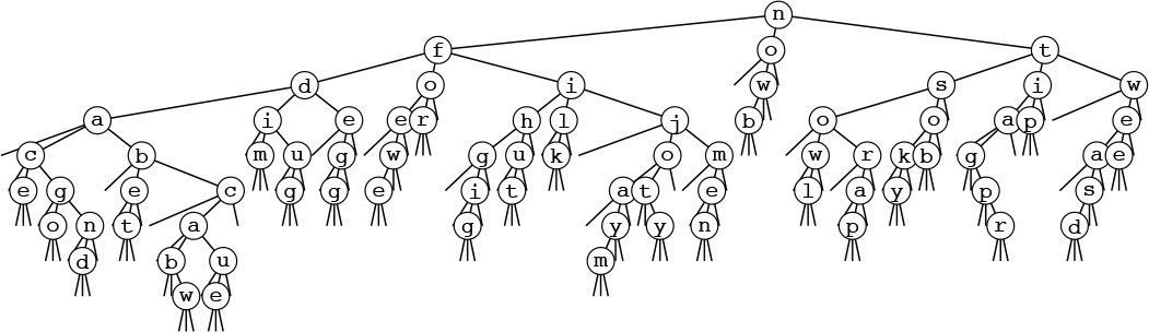
An MSD radix-sorting function divides the file on the first digit of the keys, then recursively calls itself for subfiles corresponding to each value. Figure 10.9 shows this recursive-call structure for MSD radix sorting for the example in Figure 10.8. The call structure corresponds to a multiway trie, a direct generalization of the trie structure for binary quicksort in Figure 10.4. Each node corresponds to a recursive call on the MSD sort for some subfile. For example, the subtree of the root with root labeled o corresponds to sorting the subfile consisting of the three keys of, on, and or.
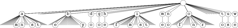
This tree corresponds to the operation of the recursive MSD radix sort in Program 10.2 on the two-letter MSD sorting example in Figure 10.8. If the file size is 1 or 0, there are no recursive calls. Otherwise, there are 26 calls: one for each possible value of the current byte.
Figure 10.9 Recursive structure of MSD radix sort.
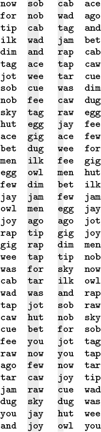
These figures make obvious the presence of significant numbers of empty bins in MSD sorting with strings. In Section 10.4, we study one way to cope with this problem; in Chapter 15, we examine explicit uses of trie structures in string-processing applications. Generally, we work with compact representations of the trie structures that do not include the nodes corresponding to the empty bins and that have the labels moved from the edges to the nodes below, as illustrated in Figure 10.10, the structure that corresponds to the recursive call structure (ignoring empty bins) for the three-letter MSD radix-sorting example of Figure 10.7. For example, the subtree of the root with root labeled j corresponds to sorting the bin containing the four keys jam, jay, jot, and joy. We examine properties of such tries in detail in Chapter 15.
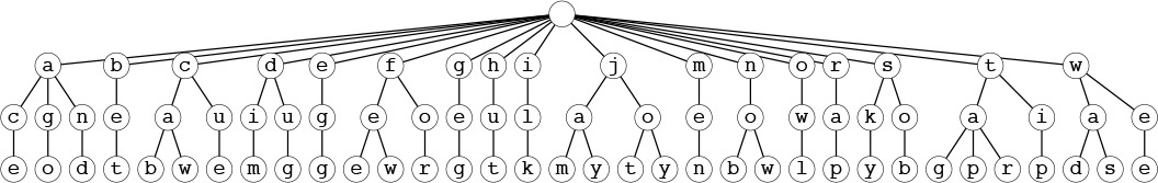
This representation of the recursive structure of MSD radix sort is more compact than the one in Figure 10.9. Each node in this tree is labeled with the value of the (i – 1)st digit of certain keys, where i is the distance from the node to the root. Each path from the root to the bottom of the tree corresponds to a key; putting the node labels together gives the key. This tree corresponds to the three-letter MSD sorting example in Figure 10.7.
Figure 10.10 Recursive structure of MSD radix sort (null subfiles ignored)
The main challenge in getting maximum efficiency in a practical MSD radix sort for keys that are long strings is to deal with lack of randomness in the data. Typically, keys may have long stretches of equal or unnecessary data, or parts of them might fall in only a narrow range. For example, an information-processing application for student data records might have keys with fields corresponding to graduation year (4 bytes, but one of four different values), state names (perhaps 10 bytes, but one of 50 different values), and gender (1 byte with one of two given values), as well as to a person’s name (more similar to random strings, but probably not short, with nonuniform letter distributions, and with trailing blanks in a fixed-length field). All these various restrictions lead to large numbers of empty bins during the MSD radix sort (see Exercise 10.23).
One practical way to cope with this problem is to develop a more complex implementation of the abstract operation of accessing bytes that takes into account any specialized knowledge that we might have about the strings being sorted. Another method that is easy to implement, which is called the bin-span heuristic, is to keep track of the high and low ends of the range of nonempty bins during the counting phase, then to use only bins in that range (perhaps also including special cases for a few special key values, such as 0 or blank). This arrangement is attractive for the kind of situation described in the previous paragraph. For example, with radix-256 alphanumeric data, we might be working with numbers in one section of the keys and thus have only 10 nonempty bins corresponding to the digits, while we might be working with uppercase letters in another section of the keys and thus have only 26 nonempty bins corresponding to them.
There are various alternatives that we might try for extending the bin-span heuristic (see reference section). For example, we could consider keeping track of the nonempty bins in an auxiliary data structure, and only keep counters and do the recursive calls for those. Doing so (and even the bin-span heuristic itself) is probably overkill for this situation, however, because the cost savings is negligible unless the radix is huge or the file size is tiny, in which case we should be using a smaller radix or sorting the file with some other method. We might achieve some of the same cost savings that we could achieve by adjusting the radix or switching to a different method for small files by using an ad hoc method, but we could not do so as easily. In Section 10.4, we shall consider yet another version of quicksort that does handle the empty-bin problem gracefully.
Exercises
![]() 10.14 Draw the compact trie strucure (with no empty bins and with keys in nodes, as in Figure 10.10) corresponding to Figure 10.9.
10.14 Draw the compact trie strucure (with no empty bins and with keys in nodes, as in Figure 10.10) corresponding to Figure 10.9.
![]() 10.15 How many nodes are there in the full trie corresponding to Figure 10.10?
10.15 How many nodes are there in the full trie corresponding to Figure 10.10?
![]() 10.16 Show how the set of keys
10.16 Show how the set of keys now is the time for all good people to come the aid of their party is partitioned with MSD radix sort.
![]() 10.17 Write a program that does four-way partitioning in place, by counting the frequency of occurrence of each key as in key-indexed counting, then using a method like Program 6.14 to move the keys.
10.17 Write a program that does four-way partitioning in place, by counting the frequency of occurrence of each key as in key-indexed counting, then using a method like Program 6.14 to move the keys.
![]() 10.18 Write a program to solve the general R-way partitioning problem, using the method sketched in Exercise 10.17.
10.18 Write a program to solve the general R-way partitioning problem, using the method sketched in Exercise 10.17.
10.19 Write a program that generates random 80-byte keys. Use this key generator to generate N random keys, then sort them with MSD radix sort, for N = 103, 104, 105, and 106. Instrument your program to print out the total number of key bytes examined for each sort.
![]() 10.20 What is the rightmost key byte position that you would expect the program in Exercise 10.19 to access for each of the given values of N? If you have done that exercise, instrument your program to keep track of this quantity, and compare your theoretical result with empirical results.
10.20 What is the rightmost key byte position that you would expect the program in Exercise 10.19 to access for each of the given values of N? If you have done that exercise, instrument your program to keep track of this quantity, and compare your theoretical result with empirical results.
10.21 Write a key generator that generates keys by shuffling a random 80-byte sequence. Use your key generator to generate N random keys, then sort them with MSD radix sort, for N = 103, 104, 105, and 106. Compare your performance results with those for the random case (see Exercise 10.19).
10.22 What is the rightmost key byte position that you would expect the program in Exercise 10.21 to access for each value of N? If you have done that exercise, compare your theoretical result with empirical results from your program.
10.23 Write a key generator that generates 30-byte random strings made up of three fields: a four-byte field with one of a set of 10 given strings; a 10-byte field with one of a set of 50 given strings; a 1-byte field with one of two given values; and a 15-byte field with random left-justified strings of letters equally likely to be four through 15 characters long. Use your key generator to generate N random keys, then sort them with MSD radix sort, for N = 103, 104, 105, and 106. Instrument your program to print out the total number of key bytes examined. Compare your performance results with those for the random case (see Exercise 10.19).
10.24 Modify Program 10.2 to implement the bin-span heuristic. Test your program on the data of Exercise 10.23.
10.4 Three-Way Radix Quicksort
Another way to adapt quicksort for MSD radix sorting is to use three-way partitioning on the leading byte of the keys, moving to the next byte on only the middle subfile (keys with leading byte equal to that of the partitioning element). This method is easy to implement (the one-sentence description plus the three-way partitioning code in Program 7.5 suffices, essentially), and it adapts well to a variety of situations. Program 10.3 is a full implementation of this method.
In essence, doing three-way radix quicksort amounts to sorting the file on the leading characters of the keys (using quicksort), then applying the method recursively on the remainder of the keys. For sorting strings, the method compares favorably with normal quicksort and with MSD radix sort. Indeed, it might be viewed as a hybrid of these two algorithms.
To compare three-way radix quicksort to standard MSD radix sort, we note that it divides the file into only three parts, so it does not get the benefit of the quick multiway partition, especially in the early stages of the sort. On the other hand, for later stages, MSD radix sort involves large numbers of empty bins, whereas three-way radix quicksort adapts well to handle duplicate keys, keys that fall into a small range, small files, and other situations where MSD radix sort might run slowly. Of particular importance is that the partitioning adapts to different types of nonrandomness in different parts of the key. Furthermore, no auxiliary array is required. Balanced against all these advantages is that extra exchanges are required to get the effect of the multiway partition via a sequence of three-way partitions when the number of subfiles is large.
Figure 10.11 shows an example of the operation of this method on the three-letter-word sorting problem of Figure 10.7. Figure 10.13 depicts the recursive-call structure. Each node corresponds to precisely three recursive calls: for keys with a smaller first byte (left child), for keys with first byte equal (middle child), and for keys with first byte larger (right child).
We divide the file into three parts: words beginning with a through i, words begininning with j, and words beginning with k through z. Then, we sort recursively.
Figure 10.11 Three-way radix quicksort
Three-way radix quicksort addresses the empty-bin problem for MSD radix sort by doing three-way partitioning to eliminate 1 byte value and (recursively) to work on the others. This action corresponds to replacing each M-way node in the trie that describes the recursive call structure of MSD radix sort (see Figure 10.9) by a ternary tree with an internal node for each nonempty bin. For full nodes (left), this change costs time without saving much space, but for empty nodes (right), the time cost is minimal and the space savings is considerable.
Figure 10.12 Example of trie nodes for three-way radix quicksort
This tree-trie combination corresponds to a substitution of the 26-way nodes in the trie in Figure 10.10 by ternary binary search trees, as illustrated in Figure 10.12. Any path from the root to the bottom of the tree that ends in a middle link defines a key in the file, given by the characters in the nodes left by middle links in the path. Figure 10.10 has 1035 null links that are not depicted; all the 155 null links in this tree are shown here. Each null link corresponds to an empty bin, so this difference illustrates how three-way partitioning can cut dramatically the number of empty bins encountered in MSD radix sorting.
Figure 10.13 Recursive structure of three-way radix quicksort
When the sort keys fit the abstraction of Section 10.2, standard quicksort (and all the other sorts in Chapters 6 through 9) can be viewed as an MSD radix sort, because the compare function has to access the most significant part of the key first (see Exercise 10.3).
For example, if the keys are strings, the compare function should access only the leading bytes if they are different, the leading 2 bytes if the first bytes are the same and the second different, and so forth. The standard algorithm thus automatically realizes some of the same performance gain that we seek in MSD radix sorting (see Section 7.7). The essential difference is that the standard algorithm cannot take special action when the leading bytes are equal. Indeed, one way to think of Program 10.3 is as a way for quicksort to keep track of what it knows about leading digits of items after they have been involved in multiple partitions. In the small subfiles, where most of the comparisons in the sort are done, the keys are likely to have many equal leading bytes. The standard algorithm has to scan over all those bytes for each comparison; the three-way algorithm avoids doing so.
Consider a case where the keys are long (and are fixed length, for simplicity), but most of the leading bytes are all equal. In such a situation, the running time of normal quicksort would be proportional to the word length times 2N ln N, whereas the running time of the radix version would be proportional to N times the word length (to discover all the leading equal bytes) plus 2N ln N (to do the sort on the remaining short keys). That is, this method could be up to a factor of ln N faster than normal quicksort, counting just the cost of comparisons. It is not unusual for keys in practical sorting applications to have characteristics similar to this artificial example (see Exercise 10.25).
Another interesting property of three-way radix quicksort is that it has no direct dependencies on the size of the radix. For other radix sorting methods, we have to maintain an auxiliary array indexed by radix value, and we need to ensure that the size of this array is not appreciably larger than the file size. For this method, there is no such table. Taking the radix to be extremely large (larger than the word size) reduces the method to normal quicksort, and taking the radix to be 2 reduces it to binary quicksort, but intermediate values of the radix give us an efficient way to deal with equal stretches among pieces of keys.
For many practical applications, we can develop a hybrid method with excellent performance by using standard MSD radix sort for large files, to get the advantage of multiway partitioning, and a three-way radix quicksort with a smaller radix for smaller files, to avoid the negative effects of large numbers of empty bins.
Three-way radix quicksort is also applicable when the keys to be sorted are vectors. That is, if the keys are made up of independent components (each an abstract key), we might wish to reorder records such that they are in order according to the first components of the keys, and in order according to the second component of the keys if the first components are equal, and so forth. We can think of vector sorting as a generalization of radix sorting where we take R to be arbitrarily large. When we adapt Program 10.3 to this application, we refer to it as multikey quicksort.
Exercises
10.25 For d > 4, suppose that keys consist of d bytes, with the final 4 bytes having random values and all the other bytes having value 0. Estimate the number of bytes examined when you sort the file using three-way radix quicksort (Program 10.3) and normal quicksort (Program 7.1) for files of size N for large N, and calculate the ratio of the running times.
10.26 Empirically determine the byte size for which three-way radix quicksort runs fastest, for random 64-bit keys with N = 103, 104, 105, and 106.
![]() 10.27 Develop an implementation of three-way radix quicksort for linked lists.
10.27 Develop an implementation of three-way radix quicksort for linked lists.
10.28 Develop an implementation of multikey quicksort for the case where the keys are vectors of t floating point numbers, using equality testing among floating point numbers as described in Exercise 4.1.
10.29 Using the key generator of Exercise 10.19, run three-way radix quicksort for N = 103, 104, 105, and 106. Compare its performance with that of MSD radix sort.
10.30 Using the key generator of Exercise 10.21, run three-way radix quicksort for N = 103, 104, 105, and 106. Compare its performance with that of MSD radix sort.
10.31 Using the key generator of Exercise 10.23, run three-way radix quicksort for N = 103, 104, 105, and 106. Compare its performance with that of MSD radix sort.
10.5 LSD Radix Sort
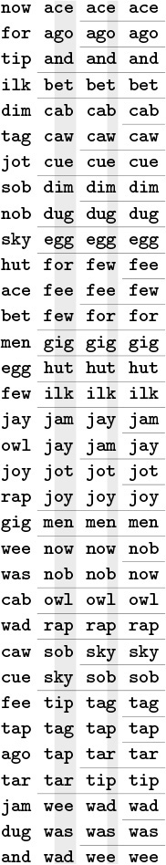
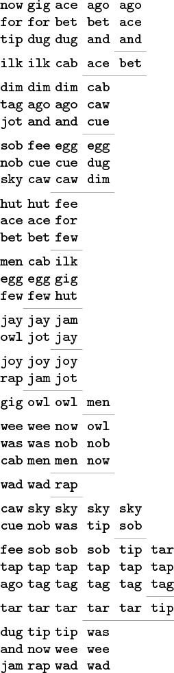
An alternative radix-sorting method is to examine the bytes from right to left. Figure 10.14 shows how our three-letter word sorting task is accomplished in just three passes through the file. We sort the file according to the final letter (using key-indexed counting), then according to the middle letter, then according to the first letter.
Three-letter words are sorted in three passes (left to right) with LSD radix sorting.
Figure 10.14 LSD radix sort example
It is not easy, at first, to be convinced that the method works; in fact, it does not work at all unless the sort method used is stable (see Definition 6.1). Once stability has been identified as being significant, a simple proof that LSD radix sorting works is easy to articulate: After putting keys into order on their i trailing bytes (in a stable manner), we know that any two keys appear in proper order (on the basis of the bits so far examined) in the file either because the first of their i trailing bytes are different, in which case the sort on that byte put them in the proper order, or because the first of their ith trailing bytes are the same, in which case they are in proper order because of stability. Stated another way, if the w – i bytes that have not been examined for a pair of keys are identical, any difference between the keys is restricted to the i bytes already examined, and the keys have been properly ordered, and will remain so because of stability. If, on the other hand, the w – i bytes that have not been examined are different, the i bytes already examined do not matter, and a later pass will correctly order the pair based on the more-significant differences.
This program implements key-indexed counting on the bytes in the words, moving right to left. The key-indexed counting implementation must be stable. If R is 2 (and therefore bytesword and bitsword are the same), this program is straight radix sort—a right-to-left bit-by-bit radix sort (see Figure 10.15).
void radixLSD(Item a[], int l, int r)
{
int i, j, w, count[R+1];
for (w = bytesword-1; w >= 0; w--)
{
for (j = 0; j < R; j++) count[j] = 0;
for (i = l; i <= r; i++)
count[digit(a[i], w) + 1]++;
for (j = 1; j < R; j++)
count[j] += count[j-1];
for (i = l; i <= r; i++)
aux[count[digit(a[i], w)]++] = a[i];
for (i = l; i <= r; i++) a[i] = aux[i-l];
}
}
This diagram depicts a right-to-left bit-by-bit radix sort working on our file of sample keys. We compute the ith column from the (i – 1)st column by extracting (in a stable manner) all the keys with a 0 in the ith bit, then all the keys with a 1 in the ith bit. If the (i – 1)st column is in order on the trailing (i – 1) bits of the keys before the operation, then the ith column is in order on the trailing i bits of the keys after the operation. The movement of the keys in the third stage is indicated explicitly.
Figure 10.15 LSD (binary) radix sort example (key bits exposed)
The stability requirement means, for example, that the partitioning method used for binary quicksort could not be used for a binary version of this right-to-left sort. On the other hand, key-indexed counting is stable, and immediately leads to a classic and efficient algorithm. Program 10.4 is an implementation of this method. An auxiliary array for the distribution seems to be required—the technique of Exercises 10.17 and 10.18 for doing the distribution in place sacrifices stability to avoid using the auxiliary array.
LSD radix sorting is the method used by old computer-card–sorting machines. Such machines had the capability of distributing a deck of cards among 10 bins, according to the pattern of holes punched in the selected columns. If a deck of cards had numbers punched in a particular set of columns, an operator could sort the cards by running them through the machine on the rightmost digit, then picking up and stacking the output decks in order, then running them through the machine on the next-to-rightmost digit, and so forth, until getting to the first digit. The physical stacking of the cards is a stable process, which is mimicked by key-indexed counting sort. Not only was this version of LSD radix sorting important in commercial applications in the 1950s and 1960s, but it was also used by many cautious programmers, who would punch sequence numbers in the final few columns of a program deck so as to be able to put the deck back in order mechanically if it were accidentally dropped.
Figure 10.15 depicts the operation of binary LSD radix sort on our sample keys, for comparison with Figure 10.3. For these 5-bit keys, the sort is completed in five passes, moving right to left through the keys. Sorting records with single-bit keys amounts to partitioning the file such that all the records with 0 keys appear before all the records with 1 keys. As just mentioned, we cannot use the partitioning strategy that we discussed at the beginning of this chapter in Program 10.1, even though it seems to solve this same problem, because it is not stable. It is worthwhile to look at radix-2 sorting, because it is often appropriate for high-performance machines and special-purpose hardware (see Exercise 10.38). In software, we use as many bits as we can to reduce the number of passes, limited only by the size of the array for the counts (see Figure 10.16).
This diagram shows the stages of LSD radix sort on random 8-bit keys, for both radix 2 (left) and radix 4, which comprises every other stage from the radix-2 diagram (right). For example, when two bits remain (second-to-last stage on the left, next-to-last stage on the right), the file consists of four intermixed sorted subfiles consisting of the keys beginning with 00, 01, 10, and 11.
Figure 10.16 Dynamic characteristics of LSD radix sort
It is typically difficult to apply the LSD approach to a string-sorting application because of variable-length keys. For MSD sorting, it is simple enough to distinguish keys according to their leading bytes, but LSD sorting is based on a fixed-length key, with the leading keys getting involved for only the final pass. Even for (long) fixed-length keys, LSD radix sorting would seem to be doing unnecessary work on the right parts of the keys, since, as we have seen, only the left parts of the keys are typically used in the sort. We shall see a way to address this problem in Section 10.7, after we have examined the properties of radix sorts in detail.
Exercises
10.32 Using the key generator of Exercise 10.19, run LSD radix sort for N = 103, 104, 105, and 106. Compare its performance with that of MSD radix sort.
10.33 Using the key generators of Exercises 10.21 and 10.23, run LSD radix sort for N = 103, 104, 105, and 106. Compare its performance with that of MSD radix sort.
10.34 Show the (unsorted) result of trying to use an LSD radix sort based on the binary quicksort partitioning method for the example of Figure 10.15.
![]() 10.35 Show the result of using LSD radix sort on the leading two characters for the set of keys
10.35 Show the result of using LSD radix sort on the leading two characters for the set of keys now is the time for all good people to come the aid of their party.
![]() 10.36 Develop an implementation of LSD radix sort using linked lists.
10.36 Develop an implementation of LSD radix sort using linked lists.
![]() 10.37 Find an efficient method that (i) rearranges the records of a file such that all those whose keys begin with a 0 bit come before all those whose keys begin with a 1 bit, (ii) uses extra space proportional to the square root of the number of records (or less), and (iii) is stable.
10.37 Find an efficient method that (i) rearranges the records of a file such that all those whose keys begin with a 0 bit come before all those whose keys begin with a 1 bit, (ii) uses extra space proportional to the square root of the number of records (or less), and (iii) is stable.
![]() 10.38 Implement a routine that sorts an array of 32-bit words using only the following abstract operation: Given a bit position i and a pointer into the array
10.38 Implement a routine that sorts an array of 32-bit words using only the following abstract operation: Given a bit position i and a pointer into the array a[k], rearrange a[k], a[k+1], ..., a[k+63] in a stable manner such that those words with a 0 bit in position i appear before those words with a 1 bit in position i.
10.6 Performance Characteristics of Radix Sorts
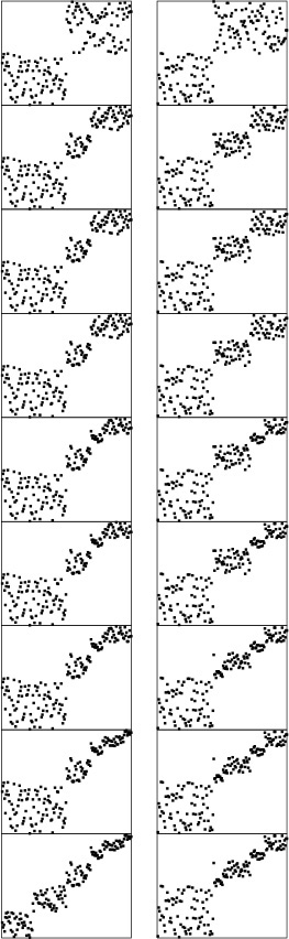
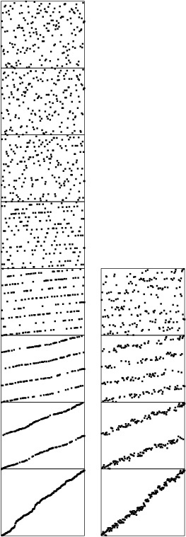
The running time of LSD radix sort for sorting N records with w-byte keys is proportional to Nw, because the algorithm makes w passes over all N keys. This analysis does not depend on the input, as illustrated in Figure 10.17.
These diagrams illustrate the stages of LSD radix sort for files of size 700 that are random, Gaussian, nearly ordered, nearly reverse ordered, and randomly ordered with 10 distinct key values (left to right). The running time is insensitive to the initial order of the input. The three files that contain the same set of keys (the first, third, and fourth all are a permutation of the integers from 1 to 700) have similar characteristics near the end of the sort.
Figure 10.17 Dynamic characteristics of LSD radix sort on various types of files
For long keys and short bytes, this running time is comparable to N lg N: For example, if we are using a binary LSD radix sort to sort 1 billion 32-bit keys, then w and lg N are both about 32. For shorter keys and longer bytes this running time is comparable to N:
For example, if a 16-bit radix is used on 64-bit keys, then w will be 4, a small constant.
To compare properly the performance of radix sort with the performance of comparison-based algorithms, we need to account carefully for the bytes in the keys, rather than for only the number of keys.
Property 10.1 The worst case for radix sorting is to examine all the bytes in all the keys.
In other words, the radix sorts are linear in the sense that the time taken is at most proportional to the number of digits in the input. This observation follows directly from examination of the programs: No digit is examined more than once. This worst case is achieved, for all the programs we have examined, when all the keys are equal. ![]()
As we have seen, for random keys and for many other situations, the running time of MSD radix sorting can be sublinear in the total number of data bits, because the whole key does not necessarily have to be examined. The following classical result holds for arbitrarily long keys:
Property 10.2 Binary quicksort examines about N lg N bits, on average, when sorting keys composed of random bits.
If the file size is a power of 2 and the bits are random, then we expect one-half of the leading bits to be 0 and one-half to be 1, so the recurrence CN = 2CN/2 + N should describe the performance, as we argued for quicksort in Chapter 7. Again, this description of the situation is not entirely accurate, because the partition falls in the center only on the average (and because the number of bits in the keys is finite). However, the partition is much more likely to be near the center for binary quicksort than for standard quicksort, so the leading term of the running time is the same as it would be were the partitions perfect. The detailed analysis that proves this result is a classical example in the analysis of algorithms, first done by Knuth before 1973 (see reference section). ![]()
This result generalizes to apply to MSD radix sort. However, since our interest is generally in the total running time, rather than in only the key characters examined, we have to exercise caution, because part of the running time of MSD radix sort is proportional to the size of the radix R and has nothing to do with the keys.
Property 10.3 MSD radix sort with radix R on a file of size N requires at least 2N + 2R steps.
MSD radix sort involves at least one key-indexed counting pass, and key-indexed counting consists of at least two passes through the records (one for counting and one for distributing), accounting for at least 2N steps, and two passes through the counters (one to initialize them to 0 at the beginning and one to determine where the subfiles are at the end), accounting for at least 2R steps. ![]()
This property almost seems too obvious to state, but it is essential to our understanding of MSD radix sort. In particular, it tells us that we cannot conclude that the running time will be low from the fact that N is small, because R could be much larger than N. In short, some other method should be used for small files. This observation is a solution to the empty-bins problem that we discussed at the end of Section 10.3. For example, if R is 256 and N is 2, MSD radix sort will be up to 128 times slower than the simpler method of just comparing elements. The recursive structure of MSD radix sort ensures that the recursive program will call itself for large numbers of small files. Therefore, ignoring the empty-bins problem could make the whole radix sort up to 128 times slower than it could be for this example. For intermediate situations (for example, suppose that R is 256 and N is 64), the cost is not so catastrophic, but is still significant. Using insertion sort is not wise, because its expected cost of N2/4 comparisons is too high; ignoring the empty bins is not wise, because there are significant numbers of them. The simplest way to cope with this problem is to use a radix that is less than the file size.
Property 10.4 If the radix is always less than the file size, the number of steps taken by MSD radix sort is within a small constant factor of N logR N on the average (for keys comprising random bytes), and within a small constant factor of the number of bytes in the keys in the worst case.
The worst-case result follows directly from the preceding discussion, and the analysis cited for Property 10.2 generalizes to give the average-case result. For large R, the factor logR N is small, so the total time is proportional to N for practical purposes. For example, if R = 216, then logR N is less than 3 for all N < 248, which value certainly encompasses all practical file sizes. ![]()
As we do from Property 10.2 we have from Property 10.4 the important practical implication that MSD radix sorting is actually a sublinear function of the total number of bits for random keys that are not short. For example, sorting 1 million 64-bit random keys will require examining only the leading 20 to 30 bits of the keys, or less than one-half of the data.
Property 10.5 Three-way radix quicksort uses 2N ln N byte comparisons, on the average, to sort N (arbitrarily long) keys.
There are two instructive ways to understand this result. First, considering the method to be equivalent to quicksort partitioning on the leading byte, then (recursively) using the same method on the subfiles, we should not be surprised that the total number of operations is about the same as for normal quicksort—but they are single-byte comparisons, not full-key comparisons. Second, considering the method from the point of view depicted in Figure 10.12, we expect that the N logR N running time from Property 10.3 should be multiplied by a factor of 2 ln R because it takes quicksort 2R ln R steps to sort R bytes, as opposed to the R steps for the same bytes in the trie. We omit the full proof (see reference section). ![]()
Property 10.6 LSD radix sort can sort N records with w-bit keys in w/ lg R passes, using extra space for R counters (and a buffer for rearranging the file).
Proof of this fact is straightforward from the implementation. In particular, if we take R = 2w/4, we get a four-pass linear sort. ![]()
Exercises
10.39 Suppose that an input file consists of 1000 copies of each of the numbers 1 through 1000, each in a 32-bit word. Describe how you would take advantage of this knowledge to get a fast radix sort.
10.40 Suppose that an input file consists of 1000 copies of each of a thousand different 32-bit numbers. Describe how you would take advantage of this knowledge to get a fast radix sort.
10.41 What is the total number of bytes examined by three-way radix quicksort when sorting fixed-length bytestrings, in the worst case?
10.42 Empirically compare the number of bytes examined by three-way radix quicksort for long strings with N = 103, 104, 105, and 106 with the number of comparisons used by standard quicksort for the same files.
![]() 10.43 Give the number of bytes examined by MSD radix sort and three-way radix quicksort for a file of N keys A, AA, AAA, AAAA, AAAAA, AAAAAA, ... .
10.43 Give the number of bytes examined by MSD radix sort and three-way radix quicksort for a file of N keys A, AA, AAA, AAAA, AAAAA, AAAAAA, ... .
10.7 Sublinear-Time Sorts
The primary conclusion that we can draw from the analytic results of Section 10.6 is that the running time of radix sorts can be sublinear in the total amount of information in the keys. In this section, we consider practical implications of this fact.
The LSD radix-sort implementation given in Section 10.5 makes bytesword passes through the file. By making R large, we get an efficient sorting method, as long as N is also large and we have space for R counters. As mentioned in the proof of Property 10.5, a reasonable choice is to make lg R (the number of bits per byte) about one-quarter of the word size, so that the radix sort is four key-indexed counting passes. Each byte of each key is examined, but there are only four digits per key. This example corresponds directly to the architectural organization of many computers: one typical organization has 32-bit words, each consisting of four 8-bit bytes. We extract bytes, rather than bits, from words, which approach is likely to be much more efficient on many computers. Now, each key-indexed–counting pass is linear, and, because there are only four of them, the entire sort is linear—certainly the best performance we could hope for in a sort.
In fact, it turns out that we can get by with only two key-indexed counting passes. We do so by taking advantage of the fact that the file will be almost sorted if only the leading w/2 bits of the w-bit keys are used. As we did with quicksort, we can complete the sort efficiently by using insertion sort on the whole file afterward. This method is a trivial modification to Program 10.4. To do a right-to-left sort using the leading one-half of the keys, we simply start the outer for loop at bytesword/2-1, rather than bytesword-1. Then, we use a conventional insertion sort on the nearly ordered file that results. Figures 10.3 and 10.18 provide convincing evidence that a file sorted on its leading bits is well ordered. Insertion sort would use only six exchanges to sort the file in the fourth column of Figure 10.3, and Figure 10.18 shows that a larger file sorted on only the leading one-half of its bits also could be sorted efficiently by insertion sort.
When keys are random bits, sorting the file on the leading bits of the keys brings it nearly into order. This diagram compares a six-pass LSD radix sort (left) on a file of random 6-bit keys with a three-pass LSD radix sort, which can be followed by an insertion-sort pass (right). The latter strategy is nearly twice as fast.
Figure 10.18 Dynamic characteristics of LSD radix sort on MSD bits
For some file sizes, it might make sense to use the extra space that would otherwise be used for the auxiliary array to try to get by with just one key-indexed–counting pass, doing the rearrangement in place. For example, sorting 1 million random 32-bit keys could be done with one key-indexed–counting sort on the leading 20 bits, then an insertion sort. To do that, we need space just for the (1 million) counters—significantly less than would be needed for an auxiliary array. Using this method is equivalent to using standard MSD radix sort with R = 220, although it is essential that a small radix be used for small files for such a sort (see the discussion after Property 10.4).
The LSD approach to radix sorting is widely used, because it involves extremely simple control structures and its basic operations are suitable for machine-language implementation, which can directly adapt to special-purpose high-performance hardware. In such an environment, it might be fastest to run a full LSD radix sort. If we use pointers, then we need to have space for N links (and R counters) to use LSD radix sort, and this investment yields a method that can sort random files with only three or four passes.
In conventional programming environments, the inner loop of the key-indexed–counting program on which the radix sorts are based contains a substantially higher number of instructions than do the inner loops of quicksort or mergesort. This property of the implementations implies that the sublinear methods that we have been describing may not be as much faster than quicksort (say) as we might expect in many situations.
General-purpose algorithms such as quicksort are more widely used than radix sort, because they adapt to a broader variety of applications. The primary reason for this state of affairs is that the key abstraction on which radix sort is built is less general than the one that we used (with the compare function) in Chapters 6 through 9. For example, one typical way to arrange the interface for a sort utility is to have the client provide the comparison function. This is the interface used by the C library qsort. This arrangement not only handles situations where the client can use specialized knowledge about complex keys to implement a fast comparison, but also allows us to sort using an ordering relation that may not involve keys at all. We examine such an algorithm in Chapter 21.
When any of them could be used, the choice among quicksort and the various radix sort algorithms (and related versions of quicksort!) that we have considered in this chapter will depend not only on features of the application (such as key, record, and file size) but also on features of the programming and machine environment that relate to the efficiency of access and use of individual bits and bytes. Tables 10.1 and 10.2 give empirical results in support of the conclusion that the linear- and sublinear-time performance results that we have discussed for various applications of radix sorts make these sorting methods an attractive choice for a variety of suitable applications.
These relative timings for radix sorts on random files of N 32-bit integers (all with a cutoff to insertion sort for N less than 16) indicate that radix sorts can be among the fastest sorts available, used with care. If we use a huge radix for tiny files, we ruin the performance of MSD radix sort, but adapting the radix to be less than the file size cures this problem. The fastest method for integer keys is LSD radix sort on the leading one-half of the bits, which we can speed up further by paying careful attention to the inner loop (see Exercise 10.45).
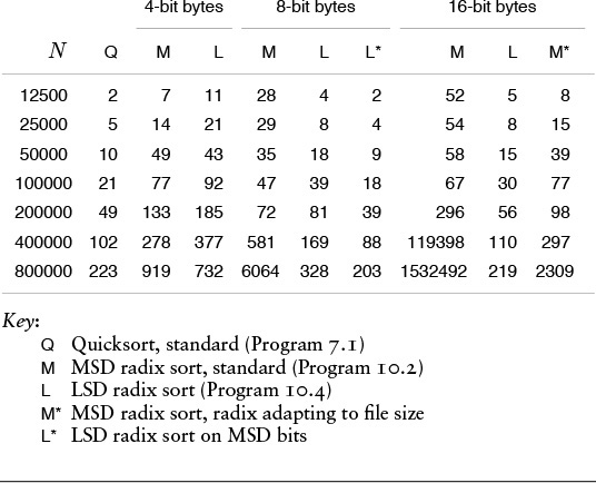
Table 10.1 Empirical study of radix sorts (integer keys)
These relative timings for various sorts on the first N words of Moby Dick (all, except heapsort, with a cutoff to insertion sort for N less than 16) indicate that the MSD-first approach is effective for string data. The cutoff for small subfiles is less effective for three-way radix quicksort than for the other methods, and is not effective at all unless we modify the insertion sort to avoid going through the leading parts of the keys (see Exercise 10.46).
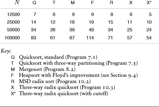
Table 10.2 Empirical study of radix sorts (string keys)
Exercises
![]() 10.44 What is the major drawback of doing LSD radix sorting on the leading bits of the keys, then cleaning up with insertion sort afterward?
10.44 What is the major drawback of doing LSD radix sorting on the leading bits of the keys, then cleaning up with insertion sort afterward?
![]() 10.45 Develop an implementation of LSD radix sort for 32-bit keys with as few instructions as possible in the inner loop.
10.45 Develop an implementation of LSD radix sort for 32-bit keys with as few instructions as possible in the inner loop.
10.46 Implement three-way radix quicksort such that the insertion sort for small files does not use leading bytes that are known to be equal in comparisons.
10.47 Given 1 million random 32-bit keys, find the choice of byte size that minimizes the total running time when we use the method of using LSD radix sort on the first two bytes, then using insertion sort to clean up.
10.48 Answer Exercise 10.47 for 1 billion 64-bit keys.
10.49 Answer Exercise 10.48 for three-pass LSD radix sort.