
CHAPTER 11
A HIERARCHY OF FORMAL LANGUAGES AND AUTOMATA
CHAPTER SUMMARY
In this chapter, we study the connection between Turing machines and languages. Depending on how one defines language acceptance, we get several different language families: recursive, recursively enumerable, and context-sensitive languages. With regular and context-free languages, these form a properly nested relation called the Chomsky hierarchy.
We now return our attention to our main interest, the study of formal languages. Our immediate goal will be to examine the languages associated with Turing machines and some of their restrictions. Because Turing machines can perform any kind of algorithmic computation, we expect to find that the family of languages associated with them is quite broad. It includes not only regular and context-free languages, but also the various examples we have encountered that lie outside these families. The nontrivial question is whether there are any languages that are not accepted by some Turing machine. We will answer this question first by showing that there are more languages than Turing machines, so that there must be some languages for which there are no Turing machines. The proof is short and elegant, but nonconstructive, and gives little insight into the problem. For this reason, we will establish the existence of languages not recognizable by Turing machines through more explicit examples that actually allow us to identify one such language. Another avenue of investigation will be to look at the relation between Turing machines and certain types of grammars and to establish a connection between these grammars and regular and context-free grammars. This leads to a hierarchy of grammars and through it to a method for classifying language families. Some set-theoretic diagrams illustrate the relationships between various language families clearly.
Strictly speaking, many of the arguments in this chapter are valid only for languages that do not include the empty string. This restriction arises from the fact that Turing machines, as we have defined them, cannot accept the empty string. To avoid having to rephrase the definition or having to add a repeated disclaimer, we make the tacit assumption that the languages discussed in this chapter, unless otherwise stated, do not contain λ. It is a trivial matter to restate everything so that λ is included, but we will leave this to the reader.
11.1 RECURSIVE AND RECURSIVELY ENUMERABLE LANGUAGES
We start with some terminology for the languages associated with Turing machines. In doing so, we must make the important distinction between languages for which there exists an accepting Turing machine and languages for which there exists a membership algorithm. Because a Turing machine does not necessarily halt on input that it does not accept, the first does not imply the second.
A language L is said to be recursively enumerable if there exists a Turing machine that accepts it.
This definition implies only that there exists a Turing machine M, such that, for every w ∈ L,
with qf a final state. The definition says nothing about what happens for w not in L; it may be that the machine halts in a nonfinal state or that it never halts and goes into an infinite loop. We can be more demanding and ask that the machine tell us whether or not any given input is in its language.
A language L on Σ is said to be recursive if there exists a Turing machine M that accepts L and that halts on every w in Σ+. In other words, a language is recursive if and only if there exists a membership algorithm for it.
If a language is recursive, then there exists an easily constructed enumeration procedure. Suppose that M is a Turing machine that determines membership in a recursive language L. We first construct another Turing machine, say , that generates all strings in Σ+ in proper order, let us say w1,w2, .... As these strings are generated, they become the input to M, which is modified so that it writes strings on its tape only if they are in L.
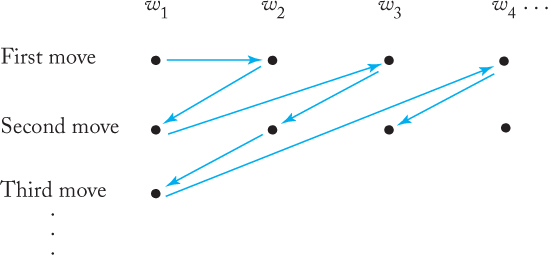
That there is also an enumeration procedure for every recursively enumerable language is not as easy to see. We cannot use the previous argument as it stands, because if some wj is not in L, the machine M, when started with wj on its tape, may never halt and therefore never get to the strings in L that follow wj in the enumeration. To make sure that this does not happen, the computation is performed in a different way. We first get to generate w1 and let M execute one move on it. Then we let generate w2 and let M execute one move on w2, followed by the second move on w1. After this, we generate w3 and do one step on w3, the second step on w2, the third step on w1, and so on. The order of performance is depicted in Figure 11.1. From this, it is clear that M will never get into an infinite loop. Since any w ∈ L is generated by and accepted by M in a finite number of steps, every string in L is eventually produced by M.
It is easy to see that every language for which an enumeration procedure exists is recursively enumerable. We simply compare the given input string against successive strings generated by the enumeration procedure. If w ∈ L, we will eventually get a match, and the process can be terminated.
Definitions 11.1 and 11.2 give us very little insight into the nature of either recursive or recursively enumerable languages. These definitions attach names to language families associated with Turing machines, but shed no light on the nature of representative languages in these families. Nor do they tell us much about the relationships between these languages or their connection to the language families we have encountered before. We are therefore immediately faced with questions such as “Are there languages that are recursively enumerable but not recursive?” and “Are there languages, describable somehow, that are not recursively enumerable?” While we will be able to supply some answers, we will not be able to produce very explicit examples to illustrate these questions, especially the second one.
Languages That Are Not Recursively Enumerable
We can establish the existence of languages that are not recursively enumerable in a variety of ways. One is very short and uses a very fundamental and elegant result of mathematics.
Let S be an infinite countable set. Then its powerset 2S is not countable.
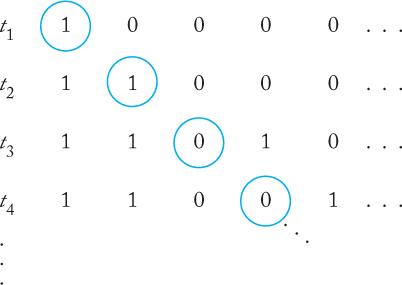
Proof: Let S = {s1,s2,s3, ...}. Then any element t of 2S can be represented by a sequence of 0’s and 1’s, with a 1 in position i if and only if si is in t. For example, the set {s2, s3, s6} is represented by 01100100..., while {s1, s3,s5, ...} is represented by 10101.... Clearly, any element of 2S can be represented by such a sequence, and any such sequence represents a unique element of 2S. Suppose that 2S were countable; then its elements could be written in some order, say t1,t2, ..., and we could enter these into a table, as shown in Figure 11.2. In this table, take the elements in the main diagonal, and complement each entry, that is, replace 0 with 1, and vice versa. In the example in Figure 11.2, the elements are 1100..., so we get 0011... as the result. The new sequence along the diagonal represents some element of 2S, say ti for some i. But it cannot be t1 because it differs from t1 through s1. For the same reason it cannot be t2, t3, or any other entry in the enumeration. This contradiction creates a logical impasse that can be removed only by throwing out the assumption that 2S is countable.
This kind of argument, because it involves a manipulation of the diagonal elements of a table, is called diagonalization. The technique is attributed to the mathematician G. F. Cantor, who used it to demonstrate that the set of real numbers is not countable. In the next few chapters, we will see a similar argument in several contexts. Theorem 11.1 is diagonalization in its purest form.
As an immediate consequence of this result, we can show that, in some sense, there are fewer Turing machines than there are languages, so that there must be some languages that are not recursively enumerable.
For any nonempty Σ, there exist languages that are not recursively enumerable.
Proof: A language is a subset of Σ*, and every such subset is a language. Therefore, the set of all languages is exactly 2Σ*. Since Σ* is infinite, Theorem 11.1 tells us that the set of all languages on Σ is not countable. But the set of all Turing machines can be enumerated, so the set of all recursively enumerable languages is countable. By Exercise 16 at the end of this section, this implies that there must be some languages on Σ that are not recursively enumerable.
This proof, although short and simple, is in many ways unsatisfying. It is completely nonconstructive and, while it tells us of the existence of some languages that are not recursively enumerable, it gives us no feeling at all for what these languages might look like. In the next set of results, we investigate the conclusion more explicitly.
A Language That Is Not Recursively Enumerable
Since every language that can be described in a direct algorithmic fashion can be accepted by a Turing machine and hence is recursively enumerable, the description of a language that is not recursively enumerable must be indirect. Nevertheless, it is possible. The argument involves a variation on the diagonalization theme.
There exists a recursively enumerable language whose complement is not recursively enumerable.
Proof: Let Σ = {a}, and consider the set of all Turing machines with this input alphabet. By Theorem 10.3, this set is countable, so we can associate an order M1,M2, ... with its elements. For each Turing machine Mi, there is an associated recursively enumerable language L (Mi). Conversely, for each recursively enumerable language on Σ, there is some Turing machine that accepts it.
We now consider a new language L defined as follows. For each i ≥ 1, the string ai is in L if and only if ai ∈ L (Mi). It is clear that the language L is well defined, since the statement ai ∈ L (Mi), and hence ai ∈ L, must be either true or false. Next, we consider the complement of L,
(11.1) |
which is also well defined but, as we will show, is not recursively enumerable.
We will show this by contradiction, starting from the assumption that is recursively enumerable. If this is so, then there must be some Turing machine, say Mk, such that
(11.2) |
Consider the string ak. Is it in L or in ? Suppose that ak ∈ . By (11.2) this implies that
ak ∈ L (Mk).
But (11.1) now implies that
ak ∉ .
Alternatively, if we assume that ak is in L, then ak ∉ and (11.2) implies that
ak ∉ L. (Mk).
But then from (11.1) we get that
ak ∈ .
The contradiction is inescapable, and we must conclude that our assumption that is recursively enumerable is false.
To complete the proof of the theorem as stated, we must still show that L is recursively enumerable. For this we can use the known enumeration procedure for Turing machines. Given ai, we first find i by counting the number of a’s. We then use the enumeration procedure for Turing machines to find Mi. Finally, we give its description along with ai to a universal Turing machine Mu that simulates the action of M on ai. If ai is in L, the computation carried out by Mu will eventually halt. The combined effect of this is a Turing machine that accepts every ai ∈ L. Therefore, by Definition 11.1, L is recursively enumerable.
The proof of this theorem explicitly exhibits, through (11.1), a well-defined language that is not recursively enumerable. This is not to say that there is an easy, intuitive interpretation of ; it would be difficult to exhibit more than a few trivial members of this language. Nevertheless, is properly defined.
A Language That Is Recursively Enumerable but Not Recursive
Next, we show there are some languages that are recursively enumerable but not recursive. Again, we need do so in a rather roundabout way. We begin by establishing a subsidiary result.
If a language L and its complement are both recursively enumerable, then both languages are recursive. If L is recursive, then is also recursive, and consequently both are recursively enumerable.
Proof: If L and are both recursively enumerable, then there exist Turing machines M and that serve as enumeration procedures for L and , respectively. The first will produce w1,w2, ... in L, the second ... in . Suppose now we are given any w ∈ Σ+. We first let M generate w1 and compare it with w. If they are not the same, we let generate and compare again. If we need to continue, we next let M generate w2, then generate , and so on. Any w ∈ Σ+ will be generated by either M or , so eventually we will get a match. If the matching string is produced by M, w belongs to L, otherwise it is in . The process is a membership algorithm for both L and , so they are both recursive.
For the converse, assume that L is recursive. Then there exists a membership algorithm for it. But this becomes a membership algorithm for by simply complementing its conclusion. Therefore, is recursive. Since any recursive language is recursively enumerable, the proof is completed.
From this, we conclude directly that the family of recursively enumerable languages and the family of recursive languages are not identical. The language L in Theorem 11.3 is in the first but not in the second family.
There exists a recursively enumerable language that is not recursive; that is, the family of recursive languages is a proper subset of the family of recursively enumerable languages.
Proof: Consider the language L of Theorem 11.3. This language is recursively enumerable, but its complement is not. Therefore, by Theorem 11.4, it is not recursive, giving us the looked-for example.
We see from this that there are indeed well-defined languages for which one cannot construct a membership algorithm.
EXERCISES
1. Prove that the set of all real numbers is not countable.
2. Prove that the set of all languages that are not recursively enumerable is not countable.
3. Let L be a finite language. Show that then L+ is recursively enumerable. Suggest an enumeration procedure for L+.
4. Let L be a context-free language. Show that L+ is recursively enumerable and suggest an enumeration procedure for it.
5. Show that if a language is not recursively enumerable, its complement cannot be recursive.
6. Show that the family of recursively enumerable languages is closed under union.
7. Is the family of recursively enumerable languages closed under intersection?
8. Show that the family of recursive languages is closed under union and intersection.
9. Show that the families of recursively enumerable and recursive languages are closed under reversal.
10. Is the family of recursive languages closed under concatenation?
11. Prove that the complement of a context-free language must be recursive.
12. Let L1 be recursive and L2 recursively enumerable. Show that L2 − L1 is necessarily recursively enumerable.
13. Suppose that L is such that there exists a Turing machine that enumerates the elements of L in proper order. Show that this means that L is recursive.
14. If L is recursive, is it necessarily true that L+ is also recursive?
15. Choose a particular encoding for Turing machines, and with it, find one element of the language in Theorem 11.3.
16. Let S1 be a countable set, S2 a set that is not countable, and S1 ⊂ S2. Show that S2 must then contain an infinite number of elements that are not in S1.
17. In Exercise 16, show that in fact S2 − S1 cannot be countable.
18. Why does the argument in Theorem 11.1 fail when S is finite?
19. Show that the set of all irrational numbers is not countable.
11.2 UNRESTRICTED GRAMMARS
To investigate the connection between recursively enumerable languages and grammars, we return to the general definition of a grammar in Chapter 1. In Definition 1.1 the production rules were allowed to take any form, but various restrictions were later made to get specific grammar types. If we take the general form and impose no restrictions, we get unrestricted grammars.
A grammar G = (V, T, S, P) is called unrestricted if all the productions are of the form
u → v,
where u is in (V ∪ T)+ and v is in (V ∪ T)*.
In an unrestricted grammar, essentially no conditions are imposed on the productions. Any number of variables and terminals can be on the left or right, and these can occur in any order. There is only one restriction: λ is not allowed as the left side of a production.
As we will see, unrestricted grammars are much more powerful than restricted forms like the regular and context-free grammars we have studied so far. In fact, unrestricted grammars correspond to the largest family of languages so we can hope to recognize by mechanical means; that is, unrestricted grammars generate exactly the family of recursively enumerable languages. We show this in two parts; the first is quite straightforward, but the second involves a lengthy construction.
Any language generated by an unrestricted grammar is recursively enumerable.
Proof: The grammar in effect defines a procedure for enumerating all strings in the language systematically. For example, we can list all w in L such that
S ⇒ w,
that is, w is derived in one step. Since the set of the productions of the grammar is finite, there will be a finite number of such strings. Next, we list all w in L that can be derived in two steps
S ⇒ x ⇒ w,
and so on. We can simulate these derivations on a Turing machine and, therefore, have an enumeration procedure for the language. Hence it is recursively enumerable.
This part of the correspondence between recursively enumerable languages and unrestricted grammars is not surprising. The grammar generates strings by a well-defined algorithmic process, so the derivations can be done on a Turing machine. To show the converse, we describe how any Turing machine can be mimicked by an unrestricted grammar.
We are given a Turing machine M = (Q, Σ, Γ,δ,q0, □,F) and want to produce a grammar G such that L (G) = L (M). The idea behind the construction is relatively simple, but its implementation becomes notationally cumbersome.
Since the computation of the Turing machine can be described by the sequence of instantaneous descriptions
(11.3) |
we will try to arrange it so that the corresponding grammar has the property that
(11.4) |
if and only if (11.3) holds. This is not hard to do; what is more difficult to see is how to make the connection between (11.4) and what we really want, namely,
for all w satisfying (11.3). To achieve this, we construct a grammar that, in broad outline, has the following properties:
1. S can derive q0w for all w ∈ Σ+.
2. (11.4) is possible if and only if (11.3) holds.
3. When a string xqf y with qf ∈ F is generated, the grammar transforms this string into the original w.
The complete sequence of derivations is then
(11.5) |
The third step in the above derivation is the troublesome one. How can the grammar remember w if it is modified during the second step? We solve this by encoding strings so that the coded version originally has two copies of w. The first is saved, while the second is used in the steps in (11.4). When a final configuration is entered, the grammar erases everything except the saved w.
To produce two copies of w and to handle the state symbol of M (which eventually has to be removed by the grammar), we introduce variables Vab and Vaib for all a ∈ Σ ∪{□}, b ∈ Γ, and all i such that qi ∈ Q. The variable Vab encodes the two symbols a and b, while Vaib encodes a and b as well as the state qi.
The first step in (11.5) can be achieved (in the encoded form) by
(11.6) |
(11.7) |
for all a ∈ Σ. These productions allow the grammar to generate an encoded version of any string q0w with an arbitrary number of leading and trailing blanks.
For the second step, for each transition
δ (qi,c) = (qj,d,R)
of M, we put into the grammar productions
VaicVpq → VadVpjq, |
(11.8) |
for all a, p ∈ Σ ∪{□}, q ∈ Γ. For each
δ (qi,c) = (qj,d,L)
of M, we include in G
VpqVaic → VpjqVad, |
(11.9) |
for all a, p ∈ Σ ∪{□}, q ∈ Γ.
If in the second step, M enters a final state, the grammar must then get rid of everything except w, which is saved in the first indices of the V’s. Therefore, for every qj ∈ F, we include productions
Vajb → a, |
(11.10) |
for all a ∈ Σ ∪ {□}, b ∈ Γ. This creates the first terminal in the string, which then causes a rewriting in the rest by
cVab → ca, |
(11.11) |
Vabc → ac, |
(11.12) |
for all a, c ∈ Σ ∪{□}, b ∈ Γ. We need one more special production
□ → λ. |
(11.13) |
This last production takes care of the case when M moves outside that part of the tape occupied by the input w. To make things work in this case, we must first use (11.6) and (11.7) to generate
□ ... □q0w □ ... □,
representing all the tape region used. The extraneous blanks are removed at the end by (11.13).
The following example illustrates this complicated construction. Carefully check each step in the example to see what the various productions do and why they are needed.
Let M = (Q, Σ, Γ,δ,q0, □,F) be a Turing machine with
and
This machine accepts L (aa*).
Consider now the computation
(11.14) |
which accepts the string aa. To derive this string with G, we first use rules of the form (11.6) and (11.7) to get the appropriate starting string,
S ⇒ SV □□ ⇒ TV □□ ⇒ TVaaV □□ ⇒ Va0aVaaV □□.
The last sentential form is the starting point for the part of the derivation that mimics the computation of the Turing machine. It contains the original input aa □ in the sequence of first indices and the initial instantaneous description q0aa □ in the remaining indices. Next, we apply
Va0aVaa → VaaVa0a,
and
Va0aV □□ → VaaV □0□,
which are specific instances of (11.8), and
VaaV □0□ → Va1aV □□
coming from (11.9). Then the next steps in the derivation are
Va0aVaaV □□ ⇒ VaaVa0aV □□ ⇒ VaaVaaV □0□ ⇒ VaaVa1aV □□.
The sequence of first indices remains the same, always remembering the initial input. The sequence of the other indices is
0aa□, a0a□, aa0□, a1a□,
which is equivalent to the sequence of instantaneous descriptions in (11.14).
Finally, (11.10) to (11.13) are used in the last steps
VaaVa1aV□□ ⇒ VaaaV□□ ⇒ Vaaa□ ⇒ aa□ ⇒ aa.
The construction described in (11.6) to (11.13) is the basis of the proof of the following result.
For every recursively enumerable language L, there exists an unrestricted grammar G, such that L = L (G).
Proof: The construction described guarantees that
x ⊢ y,
then
e (x) ⇒ e (y),
where e (x) denotes the encoding of a string according to the given convention. By an induction on the number of steps, we can then show that
if and only if
We also must show that we can generate every possible starting configuration and that w is properly reconstructed if and only if M enters a final configuration. The details, which are not too difficult, are left as an exercise.
These two theorems establish what we set out to do. They show that the family of languages associated with unrestricted grammars is identical with the family of recursively enumerable languages.
EXERCISES
1. What language does the unrestricted grammar
S |
→ |
S1B, |
S1 |
→ |
aS1b, |
bB |
→ |
bbbB, |
aS1b |
→ |
aa, |
B |
→ |
λ |
derive?
2. Construct a Turing machine for L (01 (01)∗), then find an unrestricted grammar for it using the construction in Theorem 11.7. Give a derivation for 0101 using the resulting grammar.
3. Use the construction in Theorem 11.7 to find unrestricted grammars for the following languages:
(a) L = L(aaa∗bb∗}.
(b) L = L{(ab)∗b∗}.
(c) L = {w : na(w) = nb(w)}.
4. Consider a variation on grammars in which the starting point for any derivation can be a finite set of strings, rather than a single variable. Formalize this concept, then investigate how such grammars relate to the unrestricted grammars we have used here.
5. In Example 11.1, prove that the constructed grammar cannot generate any sentence with a b in it.
6. Give the details of the proof of Theorem 11.7.
7. Show that for every unrestricted grammar there exists an equivalent unrestricted grammar, all of whose productions have the form
u → v,
with u, v ∈ (V ∪ T)+ and |u| ≤ |v|, or
A → λ,
with A ∈ V.
8. Show that the conclusion of Exercise 7 still holds if we add the further conditions |u| ≤ 2 and |v| ≤ 2.
9. Some authors give a definition of unrestricted grammars that is not quite the same as our Definition 11.3. In this alternate definition, the productions of an unrestricted grammar are required to be of the form
x → y,
where
x ∈ (V ∪ T)∗ V (V ∪ T)∗,
and
y ∈ (V ∪ T)∗.
The difference is that here the left side must have at least one variable. Show that this alternate definition is basically the same as the one we use, in the sense that for every grammar of one type, there is an equivalent grammar of the other type.
11.3 CONTEXT-SENSITIVE GRAMMARS AND LANGUAGES
Between the restricted, context-free grammars and the general, unrestricted grammars, a great variety of “somewhat restricted” grammars can be defined. Not all cases yield interesting results; among the ones that do, the context-sensitive grammars have received considerable attention. These grammars generate languages associated with a restricted class of Turing machines, linear bounded automata, which we introduced in Section 10.5.
A grammar G = (V, T, S, P) is said to be context sensitive if all productions are of the form
x → y,
where x, y ∈ (V ∪ T)+ and
|x| ≤ |y|. |
(11.15) |
This definition shows clearly one aspect of this type of grammar; it is noncontracting, in the sense that the length of successive sentential forms can never decrease. It is less obvious why such grammars should be called context sensitive, but it can be shown (see, for example, Salomaa 1973) that all such grammars can be rewritten in a normal form in which all productions are of the form
xAy → xvy.
This is equivalent to saying that the production
A → v
can be applied only in the situation where A occurs in a context of the string x on the left and the string y on the right. While we use the terminology arising from this particular interpretation, the form itself is of little interest to us here, and we will rely entirely on Definition 11.4.
Context-Sensitive Languages and Linear Bounded Automata
As the terminology suggests, context-sensitive grammars are associated with a language family with the same name.
A language L is said to be context sensitive if there exists a context-sensitive grammar G, such that L = L (G) or L = L (G) ∪{λ}.
In this definition, we reintroduce the empty string. Definition 11.4 implies that x → λ is not allowed, so that a context-sensitive grammar can never generate a language containing the empty string. Yet, every context-free language without λ can be generated by a special case of a context-sensitive grammar, say by one in Chomsky or Greibach normal form, both of which satisfy the conditions of Definition 11.4. By including the empty string in the definition of a context-sensitive language (but not in the grammar), we can claim that the family of context-free languages is a subset of the family of context-sensitive languages.
The language L = {anbncn : n ≥ 1} is a context-sensitive language. We show this by exhibiting a context-sensitive grammar for the language. One such grammar is
S |
→ |
abc|aAbc, |
Ab |
→ |
bA, |
Ac |
→ |
Bbcc, |
bB |
→ |
Bb, |
aB |
→ |
aa|aaA. |
We can see how this works by looking at a derivation of a3b3c3.
S |
⇒ |
aAbc ⇒ abAc ⇒ abBbcc |
|
⇒ |
aBbbcc ⇒ aaAbbcc ⇒ aabAbcc |
|
⇒ |
aabbAcc ⇒ aabbBbccc |
|
⇒ |
aabBbbccc ⇒ aaBbbbccc |
|
⇒ |
aaabbbccc. |
The solution effectively uses the variables A and B as messengers. An A is created on the left, travels to the right to the first c, where it creates another b and c. It then sends the messenger B back to the left in order to create the corresponding a. The process is very similar to the way one might program a Turing machine to accept the language L.
Since the language in the previous example is not context free, we see that the family of context-free languages is a proper subset of the family of context-sensitive languages. Example 11.2 also shows that it is not an easy matter to find a context-sensitive grammar even for relatively simple examples. Often the solution is most easily obtained by starting with a Turing machine program, then finding an equivalent grammar for it. A few examples will show that, whenever the language is context sensitive, the corresponding Turing machine has predictable space requirements; in particular, it can be viewed as a linear bounded automaton.
For every context-sensitive language L not including λ, there exists some linear bounded automaton M such that L = L (M).
Proof: If L is context sensitive, then there exists a context-sensitive grammar for L−{λ}. We show that derivations in this grammar can be simulated by a linear bounded automaton. The linear bounded automaton will have two tracks, one containing the input string w, the other containing the sentential forms derived using G. A key point of this argument is that no possible sentential form can have length greater than |w|. Another point to notice is that a linear bounded automaton is, by definition, nondeterministic. This is necessary in the argument, since we can claim that the correct production can always be guessed and that no unproductive alternatives have to be pursued. Therefore, the computation described in Theorem 11.6 can be carried out without using space except that originally occupied by w; that is, it can be done by a linear bounded automaton.
If a language L is accepted by some linear bounded automaton M, then there exists a context-sensitive grammar that generates L.
Proof: The construction here is similar to that in Theorem 11.7. All productions generated in Theorem 11.7 are noncontracting except (11.13),
□ → λ.
But this production can be omitted. It is necessary only when the Turing machine moves outside the bounds of the original input, which is not the case here. The grammar obtained by the construction without this unnecessary production is noncontracting, completing the argument.
Relation Between Recursive and Context-Sensitive Languages
Theorem 11.9 tells us that every context-sensitive language is accepted by some Turing machine and is therefore recursively enumerable. Theorem 11.10 follows easily from this.
Every context-sensitive language L is recursive.
Proof: Consider the context-sensitive language L with an associated context-sensitive grammar G, and look at a derivation of w
S ⇒ x1 ⇒ x2 ⇒ ··· ⇒ xn ⇒ w.
We can assume without any loss of generality that all sentential forms in a single derivation are different; that is, xi ≠ xj for all i ≠ j. The crux of our argument is that the number of steps in any derivation is a bounded function of |w|. We know that
|xj| ≤ |xj+1|,
because G is noncontracting. The only thing we need to add is that there exist some m, depending only on G and w, such that
|xj| < |xj+m|,
for all j, with m = m (|w|) a bounded function of |V ∪ T| and |w|. This follows because the finiteness of |V ∪ T | implies that there are only a finite number of strings of a given length. Therefore, the length of a derivation of w ∈ L is at most |w| m (|w|).
This observation gives us immediately a membership algorithm for L. We check all derivations of length up to |w| m (|w|). Since the set of productions of G is finite, there are only a finite number of these. If any of them give w, then w ∈ L, otherwise it is not.
There exists a recursive language that is not context sensitive.
Proof: Consider the set of all context-sensitive grammars on T = {a, b}. We can use a convention in which each grammar has a variable set of the form
V = {V0,V1,V2, ...}.
Every context-sensitive grammar is completely specified by its productions; we can think of them as written as a single string
x1 → y1; x2 → y2; ...; xm → ym.
To this string we now apply the homomorphism
h (a) |
= |
010, |
h (b) |
= |
0120, |
h (→) |
= |
0130, |
h (;) |
= |
0140, |
h (Vi) |
= |
01i+50. |
Thus, any context-sensitive grammar can be represented uniquely by a string from L ((011*0)*). Furthermore, the representation is invertible in the sense that, given any such string, there is at most one context-sensitive grammar corresponding to it.
Let us introduce a proper ordering on {0, 1}+, so we can write strings in the order w1, w2, etc. A given string wj may not define a context-sensitive grammar; if it does, call the grammar Gj. Next, we define a language L by
L = {wi : wi defines a context-sensitive grammar Gi and wi ∉ L (Gi)}.
L is well defined and is in fact recursive. To see this, we construct a membership algorithm. Given wi, we check it to see if it defines a context-sensitive grammar Gi. If not, then wi ∉ L. If the string does define a grammar, then L (Gi) is recursive, and we can use the membership algorithm of Theorem 11.10 to find out if wi ∈ L (Gi). If it is not, then wi belongs to L.
But L is not context sensitive. If it were, there would exist some wj such that L = L (Gj). We can then ask if wj is in L (Gj). If we assume that wj ∈ L (Gj), then by definition wj is not in L. But L = L (Gj), so we have a contradiction. Conversely, if we assume that wj ∉ L (Gj), then by definition wj ∈ L and we have another contradiction. We must therefore conclude that L is not context sensitive.
The result in Theorem 11.11 indicates that linear bounded automata are indeed less powerful than Turing machines, since they accept only a proper subset of the recursive languages. It follows from the same result that linear bounded automata are more powerful than pushdown automata. Context-free languages, being generated by context-free grammars, are a subset of the context-sensitive languages. As various examples show, they are a proper subset. Because of the essential equivalence of linear bounded automata and context-sensitive languages on one hand, and pushdown automata and context-free languages on the other, we see that any language accepted by a pushdown automaton is also accepted by some linear bounded automaton, but that there are languages accepted by some linear bounded automata for which there are no pushdown automata.
EXERCISES
1. Find a context-sensitive grammar that is equivalent to the unrestricted grammar in Exercise 1, Section 11.2.
2. Find context-sensitive grammars for the following languages:
(a) L = {an+1bncn−1 : n ≥ 1}.
(b) L = {anbna2n : n ≥ 1}.
(c) L = {anbmcndm : n ≥ 1,m ≥ 1}.
(d) L = {ww : w ∈ {a, b}+}.
(e) L = {anbncndn : n ≥ 1,}.
3. Find context-sensitive grammars for the following languages:
(a) L = {w : na (w) = nb (w) = nc (w)}.
(b) L = {w : na (w) = nb (w) < nc (w)}.
4. Show that the family of context-sensitive languages is closed under union.
5. Show that the family of context-sensitive languages is closed under reversal.
6. For m in Theorem 11.10, give explicit bounds for m as a function of |w| and |V ∪ T |.
7. Without explicitly constructing it, show that there exists a context-sensitive grammar for the language L = {wuwR : w, u ∈ {a, b}+, |w| ≥ |u|}.
11.4 THE CHOMSKY HIERARCHY
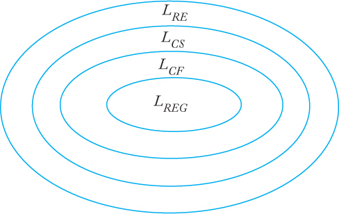
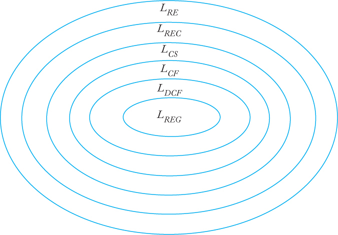
We have now encountered a number of language families, among them the recursively enumerable languages (LRE), the context-sensitive languages (LCS), the context-free languages (LCF), and the regular languages (LREG). One way of exhibiting the relationship between these families is by the Chomsky hierarchy. Noam Chomsky, a founder of formal language theory, provided an initial classification into four language types, type 0 to type 3. This original terminology has persisted and one finds frequent references to it, but the numeric types are actually different names for the language families we have studied. Type 0 languages are those generated by unrestricted grammars, that is, the recursively enumerable languages. Type 1 consists of the context-sensitive languages, type 2 consists of the context-free languages, and type 3 consists of the regular languages. As we have seen, each language family of type i is a proper subset of the family of type i − 1. A diagram (Figure 11.3) exhibits the relationship clearly. Figure 11.3 shows the original Chomsky hierarchy. We have also met several other language families that can be fitted into this picture. Including the families of deterministic context-free languages (LDCF) and recursive languages (LREC), we arrive at the extended hierarchy shown in Figure 11.4.
Other language families can be defined and their place in Figure 11.4 studied, although their relationships do not always have the neatly nested structure of Figures 11.3 and 11.4. In some instances, the relationships are not completely understood.
We have previously introduced the context-free language
L = {w : na (w) = nb (w)}
and shown that it is deterministic, but not linear. On the other hand, the language
L = {anbn} ∪ {anb2n}
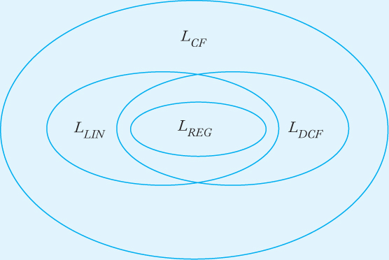
is linear, but not deterministic. This indicates that the relationship between regular, linear, deterministic context-free, and nondeterministic context-free languages is as shown in Figure 11.5.
There is still an unresolved issue. We introduced the concept of a deterministic linear bounded automaton in Exercise 8, Section 10.5. We can now ask the question we asked in connection with other automata: What role does nondeterminism play here? Unfortunately, there is no easy answer. At this time, it is not known whether the family of languages accepted by deterministic linear bounded automata is a proper subset of the context-sensitive languages.
To summarize, we have explored the relationships between several language families and their associated automata. In doing so, we established a hierarchy of languages and classified automata by their power as language accepters. Turing machines are more powerful than linear bounded automata. These in turn are more powerful than pushdown automata. At the bottom of the hierarchy are finite accepters, with which we began our study.
EXERCISES
1. Collect examples given in this book that demonstrate that all the subset relations depicted in Figure 11.4 are indeed proper ones.
2. Find two examples (excluding the one in Example 11.3) of languages that are linear but not deterministic context free.
3. Find two examples (excluding the one in Example 11.3) of languages that are deterministic context free but not linear.