CHAPTER 2

The International CAPM

Although the global CAPM (GCAPM) is the simplest risk and return model for internationally integrated financial markets, the GCAPM is not always the best model to use. You will see in this chapter that the GCAPM is a reasonable risk–return model from the US dollar perspective and perhaps from the perspective of a few other currencies as well. For many other currencies, on the other hand, one may want to apply instead the version of the international CAPM (ICAPM) introduced in this chapter.

Introduction to the Two-Factor ICAPM

Whereas the local CAPM and the GCAPM each have only one risk factor, the ICAPM version introduced in the following has two risk factors: (1) the global market index; and (2) a foreign currency index, constructed as described in the box. Because of the two risk factors, an asset has two measures of systematic risk in the ICAPM. An asset has both a “beta,” which measures sensitivity to the global market index, and a “gamma,” which measures sensitivity to the foreign currency index. The “gamma” risk coefficient (g) is called the asset’s FX exposure (to the foreign currency index).¹

The ICAPM thus involves two-factor risk premiums from the perspective of home currency H: (1) the global risk premium, GRP^H, which is the required rate of return on the global market index in currency H minus the currency-H risk-free rate, and (2) the foreign currency index risk premium, XRP^H, which is the risk premium of the foreign currency index, from the perspective of currency H, , where is the required return on the foreign currency index, inclusive of FX changes and foreign currency risk-free rates.

Each of the two ICAPM factor risk premiums is the sum of two components: (1) ; and (2) .

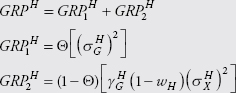
The first GRP^H component accounts for the risk in the global market index from the currency-H perspective and the aggregate market’s degree of aversion to that risk: , where Θ denotes the global market price of risk, and is the volatility (standard deviation) of the global market index return from the perspective of currency H. is the same as the global risk premium would be if the GCAPM held in currency H, or if there were no correlation between the returns on the global market index and the foreign currency index from the perspective of currency H. The second GRP^H component is: , where is the FX exposure of the global market index to the foreign currency index, which accounts for the systematic risk of the global market index versus the foreign currency index; w_H is the wealth weight of the currency-H economy; and is the volatility of the foreign currency index return.²

For example, assume Θ = 2.50 and the following inputs (shown in Exhibit 2.1) for the US dollar perspective: ; ; and . The two GRP^H components are: = 2.50[(0.1594)²] = 0.0635; and = (1 − 2.50)[1.23(1 −0.379)(0.0616)²] = −0.0043, or −0.43%. Adding the components, we get the global risk premium in US dollars: GRP^$ = 0.0635 − 0.0043 = 0.0592, or 5.92%.

For the foreign currency index risk premium, XRP^H, the first component depends on the volatility of the foreign currency index and the relative wealth weight for currency H: . The foreign currency index premium would be given a zero correlation between the returns of the global market and the foreign currency index from the perspective of currency H. The second XRP^H component accounts for any systematic risk of the foreign currency index versus the global market index, through the foreign currency index’s global beta, .

For example, assume the foreign currency index has a beta from the US dollar perspective of (as shown in Exhibit 2.1). If the US dollar is the home currency, the estimates of the two components of the foreign currency index risk premium are: = (1 − 2.50)[(1 − 0.379)(0.0616)²] = −0.0035, or −0.35%; and = 2.50[0.183(0.1594)²] = 0.0116, or 1.16%. Adding the components, the foreign currency index risk premium for the US dollar perspective is: XRP^$ = −0.0035 + 0.0116 = 0.0081, or 0.81%.

For 21 currency perspectives, Exhibit 2.1 shows the ICAPM statistical input estimates for the factor risk premium estimates, which are calculated with data for 1999 to 2016. Exhibit 2.2 shows the ICAPM’s two-factor risk premia, GRP^C and XRP^C, and the two components of each factor risk premium. The estimates assume Θ = 2.50. Note that in the ICAPM, the global market price of risk, Θ, is the same number from any currency perspective, because there is only one market price of risk in a globally integrated market.

Exhibit 2.1 ICAPM Statistical Parameter Estimates: Global Market Index and Foreign Currency Index

Note in the boxed example problem that for the Australian dollar perspective, the global risk premium estimate, 3.29%, is lower than in US dollars, 5.92%, and the foreign currency index risk premium estimate, −1.23%, is also substantially lower than the one for the US dollar perspective, 0.81%. You will better understand these differences as we explore the ICAPM further in this and subsequent chapters. You will also learn why the examples assume a global market price of risk, Θ, of 2.50.

Exhibit 2.2 ICAPM Risk Premium Estimates: Global Market Index and Foreign Currency Index

ICAPM and Cost of Capital

The traditional expression for asset i’s cost of capital in our ICAPM is the factor risk premium form shown in equation (2.1):

International CAPM (ICAPM)

Traditional Factor Risk Premium Form

In equation (2.1), and are asset i’s risk coefficients, where the prime (′) notation indicates that the risk coefficients are the partial coefficients in a multivariate regression of asset i’s return on two independent variables: (1) the global market index return, and (2) the foreign currency index return. (To simplify notation, we do not use a second subscript to denote G or X in the risk factors.) The interpretation of and is like their standard beta and FX exposure counterparts, and , except that and include adjustments for the systematic connection between the global market index and the foreign currency index.³

We now show by example that the ICAPM risk–return expression in equation (2.1) reconciles with a U.S. market index risk premium of 5.65%, using the 1999 to 2016 data and Θ = 2.50. Letting asset i be the U.S. local market index, the partial risk coefficient estimates using Excel regression and 1999 to 2016 data are: = 1.005 and = −0.353, where the U subscript denotes the U.S. equity index is asset i. Equation (2.1) says that the U.S. market risk premium should be 1.005[0.0592] − 0.353[0.0081] = 0.0565, or 5.65%.

The assumption of Θ = 2.50 for the chapter’s examples is for the deliberate purpose of “anchoring” the ICAPM illustrations to the 5.65% U.S. market risk premium estimate justified in the previous chapter.⁴ Of course, the choice of 5.65% for the U.S. market risk premium is arbitrary, but it is important to see how the various risk premium estimates, in the different currencies, are all linked by a specified global market price of risk.

Equation (2.2) shows an alternative ICAPM risk–return relation that is equivalent to the traditional expression in equation (2.1), but uses standard risk coefficients rather than the partial ones:⁵

International CAPM (ICAPM)

Standard Risk Coefficient Form

As before, is asset i’s required return in currency H, and is the currency-H risk-free rate. Instead of the more complex partial risk coeffi-cients, the risk coefficients in equation (2.2) have the standard interpretation: is asset i’s (global) beta for the currency-H perspective, and is asset i’s FX exposure to the foreign currency index for the currency-H perspective. The factor risk premiums in equation (2.2) are also not those in equation (2.1), but instead are and , the first components of GRP^H and XRP^H, respectively.

To illustrate the ICAPM risk–return expression in equation (2.2), again let asset i be the U.S. market index, and replace the i subscript with U. The U.S. market index’s global beta estimate, , is 0.939, and the U.S. market index’s estimated FX exposure to the foreign currency index, , is 0.887 (per Exhibit 2.3). Using the and estimates per Exhibit 2.2, equation (2.2) gives the U.S. market risk premium estimate: = 0.939[0.0635] + 0.887[−0.0035] = 0.0565, or 5.65%, as found using equation (2.1).

The ICAPM traditional factor risk premium form in equation (2.1) is more well-known than the standard risk coefficient form in equation (2.2). However, the benefit of using equation (2.2) is the specification in terms of standard beta and FX exposure inputs, as opposed to the partial beta and FX exposure measures in equation (2.1). This feature makes equation (2.2) advantageous for analyses in subsequent chapters.

ICAPM Versus GCAPM

The ICAPM is a theoretically stronger international risk–return model than the GCAPM, but as you have seen, the ICAPM is more complex than the GCAPM. So, a natural question is how much difference does it make in required return estimates if one uses the simpler GCAPM instead of the more complex, but theoretically superior ICAPM.

Using the “correct” (ICAPM) global risk premium estimate in US dollars (5.92%), and the local U.S. market index’s global beta estimate, 0.939, the GCAPM estimate for the U.S. local market risk premium is 0.939[0.0592] = 0.0556, or 5.56%, which is reasonably close to the “correct” (ICAPM) estimate of 5.65%. For the Australian dollar perspective, on the other hand, if one uses the “correct” (ICAPM) global risk premium estimate in Australian dollars (3.29%), and the Australian local market index’s global beta estimate, 0.603, the GCAPM estimate for the Australian local equity market risk premium is 0.603[0.0329] = 0.0198, or 1.98%, which is 114 basis points below the “correct” (ICAPM) estimate, 3.12%, found in the last boxed example.

For 31 local equity market indexes, including 10 individual Eurozone countries and the Eurozone in aggregate (using the EMU Index), Exhibit 2.3 compares the ICAPM and GCAPM equity market risk premium estimates in local currency for the 1999 to 2016 data. Country Y’s ICAPM market risk premium estimate is based on equation (2.2), using the estimates for the country index’s global beta, , and FX exposure to the foreign currency index, , as shown in Exhibit 2.3. The other inputs used in equation (2.2) are shown in Exhibit 2.1. Country Y’s GCAPM market risk premium estimate is equal to the country index’s global beta estimate times the local currency’s “correct” (ICAPM) global market risk premium estimate, GRP^C, per Exhibit 2.2.

Exhibit 2.3 ICAPM vs. GCAPM Local Market Risk Premium Estimates

Exhibit 2.3 shows that for three countries (in addition to the United States), the GCAPM gives a very close approximation to the “correct” (ICAPM) estimate of the country’s local equity market risk premium: Japan, China, and Hong Kong. Other countries for which the difference is under 30 basis points, and therefore where the GCAPM’s estimates may be a reasonable approximation to the ICAPM’s estimates include Britain, Switzerland, Denmark, and Ireland.

On the other hand, there are many countries where the difference between the GCAPM and “correct” (ICAPM) local market risk premium estimates is more than 60 basis points, and the difference is more than 100 basis points for eight countries: Australia, India, Korea, Brazil, Norway, South Africa, Thailand, and Austria.

Bear in mind that Country Y’s local equity market index represents Country Y’s “average stock.” The difference between the ICAPM and GCAPM cost of equity estimates for individual stocks may be higher than that for the “average stock.”

As a case in point, Exhibit 2.3 indicates the difference between the ICAPM and GCAPM risk premium estimates for the local British equity index is 25 basis points, yet the next boxed example problem shows that the difference between Rio Tinto’s ICAPM and GCAPM cost of equity estimates in British pounds is 80 basis points.

An empirical study of ICAPM and GCAPM cost of equity estimates for individual U.S. stocks for the 1985 to 2012 period found an average cost of equity difference of only 32 basis points. This average difference is relatively small, especially considering the sample included many small companies. Thus, the study’s results indicate that the simpler GCAPM may provide an acceptable approximation to the more complex ICAPM for US dollar cost of equity estimates of U.S. companies.⁶ Although there is no empirical research yet that compares ICAPM and GCAPM cost of equity estimates for individual stocks of other countries and currencies, the results in Exhibit 2.3 suggest that GCAPM cost of equity estimates are not good approximations of ICAPM estimates, on average, for many countries.

An Asset’s Required Return in Different Currencies

Just as an asset’s rate of return is different from the perspective of different currencies, per equation (1.1a), an asset’s required rate of return, or cost of capital, is different from the perspective of different currencies. So, you must be careful to specify which currency you are using to express a cost of capital. Different cost of equity numbers in different currencies are separate ways to express the same cost of equity. This idea is the same as saying that a firm’s equity has only one value, but it is a different number when expressed in different currencies. That is, you can express a firm’s equity value either as $100 or Sf 160 given a spot FX rate of 1.60 Sf/$.

Despite being different numbers, a given asset’s cost of capital estimates in different currencies must be mutually consistent with each other. To better understand what this means, say an angel were to post online the true expected future cash flow per share for BHP Billiton, and the angel provides this information from both the Australian dollar and US dollar perspectives. BHP Billiton’s cost of equity in Australian dollars must be consistent with the cost of equity in US dollars in the following way: If the $/A$ FX rate is correctly valued and expected to be correctly valued in the future, the present (discounted) value of the expected cash flows in the Australian dollar perspective is equivalent at today’s spot FX rate to the present (discounted) value of the expected cash flows in the US dollar perspective.

The theory that underlies the ICAPM implicitly assures us that the estimates of a given asset’s cost of capital in different currencies are consistent with each other. However, the GCAPM does not give consistent cross-currency cost of capital estimates; the reason is technical and beyond the scope here to cover in detail.⁷

Summary Action Points

Glossary

FX exposure: Sensitivity to changes in FX rates or an index of FX rates, like a beta but with the FX rate(s) replacing the market index.

Partial Risk Coefficients: Risk coefficients (beta and gamma) that are estimated through multiple regression and thus take into consideration the statistical connection of the risk factors.

Standard Risk Coefficients: Risk coefficients (beta and gamma) that are estimated through univariate regression and thus do not take into consideration the statistical connection of the risk factors.

International CAPM (ICAPM): A risk-return model in internationally integrated financial markets in which the global market index replaces the traditional CAPM market index and which has one or more foreign exchange FX risk factors.

Problems

Answers to Problems

Discussion Questions