
Chapter 7: Logistic Regression for Matched Case-Control Studies
7.1 Introduction
An important special case of the stratified case-control study discussed in Chapter 6 is the matched case-control study. A discussion of the rationale for matched studies may be found in epidemiology texts such as Breslow and Day (1980), Kleinbaum et al. (1982), Schlesselman (1985), Kelsey et al. (1986), and Rothman et al. (2008). In this study design, subjects are stratified on the basis of variables believed to be associated with the outcome. Age and gender are examples of commonly used stratification variables. Within each stratum, samples of cases ![]() and controls
and controls ![]() are chosen. The number of cases and controls need not be constant across strata, but the most common matched designs include one case and from 1–5 controls per stratum and are thus referred to as
are chosen. The number of cases and controls need not be constant across strata, but the most common matched designs include one case and from 1–5 controls per stratum and are thus referred to as ![]() matched studies.
matched studies.
In this chapter we develop the methods for analyzing general matched studies. We illustrate the methods for both the ![]() matched study and a
matched study and a ![]() matched study (as an example of the more general
matched study (as an example of the more general ![]() design).
design).
We begin by providing some motivation and rationale for the need for special methods for the matched study. In Chapter 6, it was noted that we could handle the stratified sample by including the design variables created from the stratification variable in the model. This approach works well when the number of subjects in each stratum is large. However, in a typical matched study we are likely to have few subjects per stratum. For example, in the ![]() matched design with
matched design with ![]() case-control pairs we have only two subjects per stratum. Thus, in a fully stratified analysis with
case-control pairs we have only two subjects per stratum. Thus, in a fully stratified analysis with ![]() covariates, we would be required to estimate
covariates, we would be required to estimate ![]() parameters consisting of the constant term, the
parameters consisting of the constant term, the ![]() slope coefficients for the covariates, and the
slope coefficients for the covariates, and the ![]() coefficients for the stratum-specific design variables using a sample of size
coefficients for the stratum-specific design variables using a sample of size ![]() . The optimality properties of the method of maximum likelihood, derived by letting the sample size become large, hold only when the number of parameters remains fixed. This is clearly not the case in any
. The optimality properties of the method of maximum likelihood, derived by letting the sample size become large, hold only when the number of parameters remains fixed. This is clearly not the case in any ![]() matched study. With the fully stratified analysis, the number of parameters increases at the same rate as the sample size. For example, with a model containing one dichotomous covariate it can be shown [see Breslow and Day (1980)] that the bias in the estimate of the coefficient is 100% when analyzing a matched
matched study. With the fully stratified analysis, the number of parameters increases at the same rate as the sample size. For example, with a model containing one dichotomous covariate it can be shown [see Breslow and Day (1980)] that the bias in the estimate of the coefficient is 100% when analyzing a matched ![]() design via a fully stratified likelihood. If we regard the stratum-specific parameters as nuisance parameters, and if we are willing to forgo their estimation, then we can use methods for conditional inference to create a likelihood function that yields maximum likelihood estimators of the slope coefficients in the logistic regression model that are consistent and asymptotically normally distributed. The mathematical details of conditional likelihood analysis may be found in Cox and Hinkley (1974).
design via a fully stratified likelihood. If we regard the stratum-specific parameters as nuisance parameters, and if we are willing to forgo their estimation, then we can use methods for conditional inference to create a likelihood function that yields maximum likelihood estimators of the slope coefficients in the logistic regression model that are consistent and asymptotically normally distributed. The mathematical details of conditional likelihood analysis may be found in Cox and Hinkley (1974).
Suppose that there are ![]() strata with
strata with ![]() cases and
cases and ![]() controls in stratum
controls in stratum ![]() . We begin with the stratum-specific logistic regression model
. We begin with the stratum-specific logistic regression model
where ![]() denotes the contribution to the logit of all terms constant within the
denotes the contribution to the logit of all terms constant within the ![]() stratum (i.e., the matching or stratification variable(s)). In this chapter, the vector of coefficients,
stratum (i.e., the matching or stratification variable(s)). In this chapter, the vector of coefficients, ![]() , contains only the
, contains only the ![]() slope coefficients,
slope coefficients, ![]() . It follows from the results in Chapter 3 that each slope coefficient gives the change in the log-odds for a one unit increase in the covariate holding all other covariates constant in every stratum. This is important to keep in mind as the steps, to be described, in developing a conditional likelihood result in a model that does not look like a logistic regression model, yet it contains the coefficient vector,
. It follows from the results in Chapter 3 that each slope coefficient gives the change in the log-odds for a one unit increase in the covariate holding all other covariates constant in every stratum. This is important to keep in mind as the steps, to be described, in developing a conditional likelihood result in a model that does not look like a logistic regression model, yet it contains the coefficient vector, ![]() . The fact that the model does not look like a logistic regression model leads new users to think that estimated coefficients must be modified in some way before they can be used to estimate odds ratios. This is not the case, and we pay particular attention in this chapter to estimation and interpretation of odds ratios.
. The fact that the model does not look like a logistic regression model leads new users to think that estimated coefficients must be modified in some way before they can be used to estimate odds ratios. This is not the case, and we pay particular attention in this chapter to estimation and interpretation of odds ratios.
The conditional likelihood for the ![]() stratum is obtained as the probability of the observed data conditional on the stratum total and the total number of cases observed, the sufficient statistic for the nuisance parameter. In this setting, it is the probability of the observed data relative to the probability of the data for all possible assignments of
stratum is obtained as the probability of the observed data conditional on the stratum total and the total number of cases observed, the sufficient statistic for the nuisance parameter. In this setting, it is the probability of the observed data relative to the probability of the data for all possible assignments of ![]() cases and
cases and ![]() controls to
controls to ![]() subjects. The number of possible assignments of case status to
subjects. The number of possible assignments of case status to ![]() subjects among the
subjects among the ![]() subjects, denoted here as
subjects, denoted here as ![]() , is given by the mathematical expression
, is given by the mathematical expression
![]()
Let the subscript ![]() denote any one of these
denote any one of these ![]() assignments. For any assignment we let subjects 1 to
assignments. For any assignment we let subjects 1 to ![]() correspond to the cases and subjects
correspond to the cases and subjects ![]() to
to ![]() to the controls. This is indexed by
to the controls. This is indexed by ![]() for the observed data and by
for the observed data and by ![]() for the
for the ![]() possible assignment. The conditional likelihood is
possible assignment. The conditional likelihood is

The full conditional likelihood is the product of the ![]() in equation 7.2 over the
in equation 7.2 over the ![]() strata, namely,
strata, namely,

If we assume that the stratum-specific logistic regression model in equation 7.1 is correct then application of Bayes' theorem to each ![]() term in equation 7.2 yields
term in equation 7.2 yields

Note that when we apply Bayes' theorem all terms of the form
![]()
appear equally in both the numerator and denominator of equation 7.2 and thus cancel out. Algebraic simplification yields the function shown in equation 7.4 where ![]() is the only unknown parameter. The conditional maximum likelihood estimator for
is the only unknown parameter. The conditional maximum likelihood estimator for ![]() is that value that maximizes equation 7.3 when
is that value that maximizes equation 7.3 when ![]() is as shown in equation 7.4. Except in one special case it is not possible to express the likelihood in equation 7.4 in a form similar to the unconditional likelihood in equation (1.3). However, as we noted earlier, the coefficients have not been modified, and thus have the same interpretation as those in equation 7.1.
is as shown in equation 7.4. Except in one special case it is not possible to express the likelihood in equation 7.4 in a form similar to the unconditional likelihood in equation (1.3). However, as we noted earlier, the coefficients have not been modified, and thus have the same interpretation as those in equation 7.1.
The most frequently used matched design is one in which each case is matched to a single control; thus, there are two subjects in each stratum. It is helpful to consider this design, not only because it is used frequently in practice, but also because it helps illustrate some key differences in the effect covariate values have on the likelihood function in equations (1.3) and 7.4. To simplify the notation, let ![]() denote the data vector for the case and
denote the data vector for the case and ![]() the data vector for the control in the
the data vector for the control in the ![]() stratum or pair. Using this notation, the conditional likelihood for the
stratum or pair. Using this notation, the conditional likelihood for the ![]() stratum from equation 7.4 is
stratum from equation 7.4 is
Given specific values for ![]() ,
, ![]() , and
, and ![]() , equation 7.5 is the probability that, within stratum
, equation 7.5 is the probability that, within stratum ![]() , the subject identified as the case is in fact the case under the assumptions that: (i) we have two subjects, one of whom is the case and (ii) the logistic regression model in equation 7.1 is the correct model. For example, suppose we have a model with a single dichotomous covariate and
, the subject identified as the case is in fact the case under the assumptions that: (i) we have two subjects, one of whom is the case and (ii) the logistic regression model in equation 7.1 is the correct model. For example, suppose we have a model with a single dichotomous covariate and ![]() and the observed data are
and the observed data are ![]() and
and ![]() then the value of equation 7.5 is
then the value of equation 7.5 is
![]()
Thus, the probability is 0.69 that a subject with ![]() is the case compared to a subject with
is the case compared to a subject with ![]() . On the other hand, if
. On the other hand, if ![]() and
and ![]() then
then
![]()
and the probability is 0.31 that a subject with ![]() is the case compared to a subject with
is the case compared to a subject with ![]() . Thus, we see that the affect of a covariate value is measured relative to the values in its matched set rather than relative to all values of the covariate, which is the case with the likelihood in equation (1.3) or its log-likelihood in equation (1.4).
. Thus, we see that the affect of a covariate value is measured relative to the values in its matched set rather than relative to all values of the covariate, which is the case with the likelihood in equation (1.3) or its log-likelihood in equation (1.4).
It also follows from equation 7.5 that if the data for the case and the control are identical, ![]() , then
, then ![]() for any value of
for any value of ![]() (i.e., the data for the case and control are equally likely under the model). Thus, case-control pairs with the same value for any covariate are uninformative for estimation of that covariate's coefficient. We use the term uninformative to describe the fact that the value of the covariate does not help distinguish which subject is more likely to be the case. This tends to occur most frequently with dichotomous covariates where common values, often called concordant pairs, are most likely to occur. A fact not discussed in this chapter, which can be found in Breslow and Day (1980), is that the maximum likelihood estimator of the coefficient for a dichotomous covariate in a univariable conditional logistic regression model fit to
(i.e., the data for the case and control are equally likely under the model). Thus, case-control pairs with the same value for any covariate are uninformative for estimation of that covariate's coefficient. We use the term uninformative to describe the fact that the value of the covariate does not help distinguish which subject is more likely to be the case. This tends to occur most frequently with dichotomous covariates where common values, often called concordant pairs, are most likely to occur. A fact not discussed in this chapter, which can be found in Breslow and Day (1980), is that the maximum likelihood estimator of the coefficient for a dichotomous covariate in a univariable conditional logistic regression model fit to ![]() matched data is the log of the ratio of discordant pairs. The practical significance of this is that the estimator may be based on a small fraction of the total number of possible pairs. We feel it is good practice to form the
matched data is the log of the ratio of discordant pairs. The practical significance of this is that the estimator may be based on a small fraction of the total number of possible pairs. We feel it is good practice to form the ![]() table cross-classifying case versus control for all dichotomous covariates in order to determine the number of discordant pairs. This is essentially a univariable logistic regression and, as we have stated previously, univariable analyses of all covariates should be among the first steps in any model building process. The reader should be aware that, if both types of pairs,
table cross-classifying case versus control for all dichotomous covariates in order to determine the number of discordant pairs. This is essentially a univariable logistic regression and, as we have stated previously, univariable analyses of all covariates should be among the first steps in any model building process. The reader should be aware that, if both types of pairs, ![]() and
and ![]() , are not present in the data, then the estimator is undefined. In this case, software packages will either remove the covariate from the model or give an impractically large coefficient and standard error. This is the same zero cell problem discussed in Section 4.5. The same type of problem can occur for polychotomous covariates, but it involves more complex relationships than simply a zero frequency cell in the cross-classification of case versus control [Breslow and Day (1980)].
, are not present in the data, then the estimator is undefined. In this case, software packages will either remove the covariate from the model or give an impractically large coefficient and standard error. This is the same zero cell problem discussed in Section 4.5. The same type of problem can occur for polychotomous covariates, but it involves more complex relationships than simply a zero frequency cell in the cross-classification of case versus control [Breslow and Day (1980)].
As a few software packages still do not have specific commands for maximizing the conditional log-likelihood, it is possible, with some data manipulation, to use a standard logistic regression package to maximize the full conditional log-likelihood for the ![]() design. We begin by re-expressing equation 7.5 by dividing its numerator and denominator by
design. We begin by re-expressing equation 7.5 by dividing its numerator and denominator by ![]() yielding
yielding

The expression on the right side of equation 7.6 is the usual logistic regression model with the constant term set equal to zero ![]() and data vector equal to the data value of the case minus the data value of the control,
and data vector equal to the data value of the case minus the data value of the control, ![]() . It follows that the full conditional likelihood may be expressed as
. It follows that the full conditional likelihood may be expressed as

where ![]() for all
for all ![]() .
.
This observation allows one to use standard logistic regression software to compute the conditional maximum likelihood estimates and obtain estimated standard errors of the estimated coefficients. To do this, one must define the sample size as the number of case-control pairs, use as covariates the differences ![]() , set the values of the response variable equal to one
, set the values of the response variable equal to one ![]() , and exclude the constant term from the model. Thus, from a computational point of view, the
, and exclude the constant term from the model. Thus, from a computational point of view, the ![]() matched design may be fit using any logistic regression program.
matched design may be fit using any logistic regression program.
Software to perform the necessary calculations using the log of the likelihood in equation 7.3 is now available in most statistical software packages. For example, STATA has a special conditional logistic regression command. With SAS and a few other packages, one must perform a simple modification of the data and perform the analysis using the package's proportional hazards regression command. The calculations for this chapter were performed in STATA.
In summary, the methods for model building for matched data are identical to those discussed and illustrated in detail for unmatched data in Chapter 4. Hence, we do not repeat them here, but illustrate them in the examples. There are, however, important differences when one assesses the fit of the model from matched data. The ideas are the same as those discussed in Chapter 5 for unmatched data, but the calculations of the diagnostic statistics are different. These are presented and discussed in the next section. We conclude the chapter with examples of using logistic regression to model data from a ![]() and a
and a ![]() design.
design.
7.2 Methods For Assessment of Fit in a 1−M Matched Study
Our approach to assessment of fit in the ![]() matched study is based on extensions of regression diagnostics for the unconditional logistic regression model. The mathematics required to develop these statistics is at a higher level than other sections of the book. Hence, less sophisticated mathematical readers may wish to skip this section and proceed to examples where the use of the diagnostic statistics is explained and illustrated. Moolgavkar et al. (1985) and Pregibon (1984) derive these diagnostic statistics for a general matched design, but only illustrate their use in the
matched study is based on extensions of regression diagnostics for the unconditional logistic regression model. The mathematics required to develop these statistics is at a higher level than other sections of the book. Hence, less sophisticated mathematical readers may wish to skip this section and proceed to examples where the use of the diagnostic statistics is explained and illustrated. Moolgavkar et al. (1985) and Pregibon (1984) derive these diagnostic statistics for a general matched design, but only illustrate their use in the ![]() matched design. STATA currently provides access to the diagnostics following the fit of a logistic model using equation 7.3. To simplify the notation somewhat we present the results for the setting when
matched design. STATA currently provides access to the diagnostics following the fit of a logistic model using equation 7.3. To simplify the notation somewhat we present the results for the setting when ![]() (i.e.,
(i.e., ![]() subjects per stratum).
subjects per stratum).
There are no easily computed goodness of fit tests for the matched data setting. Zhang (1999) discusses a test but it is not available in any software package. Arbogast and Lin (2005) propose a method based on cumulative sums of residuals within matched sets with significance and visual assessment based on simulations. Again, the method is complicated to compute and is not available in software packages.
Since the diagnostics are not computed in all software packages we describe them as if one was going to compute them following the fit of a model. The first step is to transform the observed values of the covariate vector by centering them about a weighted stratum-specific mean. That is, we compute for each stratum, ![]() , and each subject within each stratum,
, and each subject within each stratum, ![]() ,
,

where

and note that ![]() . Let
. Let ![]() be the
be the ![]() by
by ![]() matrix whose rows are the values of
matrix whose rows are the values of ![]() and
and ![]() . Let
. Let ![]() be an
be an ![]() by
by ![]() diagonal matrix with general diagonal element
diagonal matrix with general diagonal element ![]() . It may be shown that the maximum likelihood estimator,
. It may be shown that the maximum likelihood estimator, ![]() , once obtained can be re-computed via the equation
, once obtained can be re-computed via the equation
![]()
where ![]() is the vector
is the vector ![]() ,
, ![]() is the vector of values of the outcome variable (
is the vector of values of the outcome variable (![]() for the case and
for the case and ![]() for the controls), and
for the controls), and ![]() is the vector whose components are
is the vector whose components are ![]() . Recall that
. Recall that ![]() is, under the assumption of a logistic regression model, the estimated conditional probability that subject
is, under the assumption of a logistic regression model, the estimated conditional probability that subject ![]() within stratum
within stratum ![]() is a case.
is a case.
It follows from the above expression for ![]() that we may re-compute the maximum likelihood estimate for the conditional logistic regression model using a linear regression program allowing case weights. We use the vector
that we may re-compute the maximum likelihood estimate for the conditional logistic regression model using a linear regression program allowing case weights. We use the vector ![]() as values of the independent variables,
as values of the independent variables,

as the values of the dependent variable, and case weight ![]() , for
, for ![]() ,
, ![]() . It follows that the diagonal elements of the hat matrix computed by the linear regression are the leverage values we need, namely
. It follows that the diagonal elements of the hat matrix computed by the linear regression are the leverage values we need, namely
We note that the leverage values in equation 7.7 are of the same form as those in equation (5.22). Here, the “v” part is the conditional probability ![]() and the “b” part is
and the “b” part is ![]() . The “v” part is not an estimator of the variance as it is in equation (5.22). However, the leverage in equation 7.7 does go to zero as
. The “v” part is not an estimator of the variance as it is in equation (5.22). However, the leverage in equation 7.7 does go to zero as ![]() goes to zero. The “b” part will be large when the individual covariate values are different from the matched set weighted mean, as opposed to the overall mean in equation (5.21). Hence subjects with high leverage will be those whose covariate values differ from the matched set mean and have an estimated conditional probability between 0.3 and 0.7.
goes to zero. The “b” part will be large when the individual covariate values are different from the matched set weighted mean, as opposed to the overall mean in equation (5.21). Hence subjects with high leverage will be those whose covariate values differ from the matched set mean and have an estimated conditional probability between 0.3 and 0.7.
We note that one must pay close attention to how weights are handled in the statistical package used for the weighted linear regression. For example, SAS's regression procedure outputs the values as defined in equation 7.7. STATA users need to multiply the leverage values created following the weighted regression by ![]() to obtain the leverage values defined in equation 7.7, where
to obtain the leverage values defined in equation 7.7, where ![]() is the mean of the estimated logistic probabilities.
is the mean of the estimated logistic probabilities.
The Pearson residual is
and the Pearson chi-square is

Unfortunately, the large sample approach of Osius and Rojek (1992) cannot be used in this setting to obtain a standardized statistic and significance level.
The standardized Pearson residual is

In keeping with the diagnostics for the unmatched design we define the square of the standardized residual as the lack of fit diagnostic
and the influence diagnostic as
We feel that the most informative way to view the diagnostic statistics is via a plot of their values versus the fitted values, ![]() . These plots are similar to those used in Chapter 5 to assess graphically the fit of the unconditional logistic regression. Examples of these plots are presented in the next section.
. These plots are similar to those used in Chapter 5 to assess graphically the fit of the unconditional logistic regression. Examples of these plots are presented in the next section.
Moolgavkar et al. (1985) and Pregibon (1984) suggest that one should use the stratum-specific totals of the two diagnostics, ![]() and
and ![]() to assess what affect the data in an entire stratum have on the fit of the model. These statistics are computed as quadratic forms involving not only the leverage values for the subjects in the stratum, but also those terms in the hat matrix that account for the correlation among the fitted values. An easily computed approximation to these statistics is obtained by ignoring the off diagonal elements in the hat matrix. We feel that the approximations are likely to be accurate enough for practical purposes. For the
to assess what affect the data in an entire stratum have on the fit of the model. These statistics are computed as quadratic forms involving not only the leverage values for the subjects in the stratum, but also those terms in the hat matrix that account for the correlation among the fitted values. An easily computed approximation to these statistics is obtained by ignoring the off diagonal elements in the hat matrix. We feel that the approximations are likely to be accurate enough for practical purposes. For the ![]() stratum these are
stratum these are

and

Strata with large values of these statistics would be judged to be poorly fit and/or have large influence respectively. One can use a boxplot or a plot of their values versus stratum number to identify those strata with exceptionally large values. For these strata, the individual contributions to these quantities should be examined carefully to determine whether cases and/or controls are the cause of the large values.
The diagnostic statistics described in this section are similar to the diagnostics one would obtain in the ![]() matched setting by fitting the model using the difference data and computing the diagnostics shown in Chapter 5. For this reason, some users may prefer the difference data approach to the
matched setting by fitting the model using the difference data and computing the diagnostics shown in Chapter 5. For this reason, some users may prefer the difference data approach to the ![]() design. Specifically, the diagnostics based on the difference data are based on one value per stratum, while those computed from equations (7.7)–(7.9) yield two values per stratum. The mathematical relationships between the two diagnostic statistics are complex. For example, the stratum totals described in equations 7.10 and 7.11 are not arithmetically equal to the values of
design. Specifically, the diagnostics based on the difference data are based on one value per stratum, while those computed from equations (7.7)–(7.9) yield two values per stratum. The mathematical relationships between the two diagnostic statistics are complex. For example, the stratum totals described in equations 7.10 and 7.11 are not arithmetically equal to the values of ![]() and
and ![]() from Chapter 5. While it may appear that we have two different sets of values of the diagnostic statistics they do identify the same strata as being poorly fit or influential. Thus from a practical point of view one may use either the difference data or the results in this section to assess model adequacy in the
from Chapter 5. While it may appear that we have two different sets of values of the diagnostic statistics they do identify the same strata as being poorly fit or influential. Thus from a practical point of view one may use either the difference data or the results in this section to assess model adequacy in the ![]() design. In all other matched designs, one must use the diagnostics described in this section.
design. In all other matched designs, one must use the diagnostics described in this section.
In identifying poorly fit or influential subjects deletion of the case in a stratum, assuming a ![]() design, is tantamount to deletion of all subjects in the stratum. Without a case, a stratum contributes no information to the likelihood function. If some, but not all, controls are deleted in a specific stratum then the stratum may still have enough information to contribute to the likelihood function. A final decision on exclusion or inclusion of cases (entire strata) or controls should be based on the clinical plausibility of the data.
design, is tantamount to deletion of all subjects in the stratum. Without a case, a stratum contributes no information to the likelihood function. If some, but not all, controls are deleted in a specific stratum then the stratum may still have enough information to contribute to the likelihood function. A final decision on exclusion or inclusion of cases (entire strata) or controls should be based on the clinical plausibility of the data.
7.3 An Example Using the Logistic Regression Model in a  Matched Study
For illustrative purposes we created a ![]() matched data set from the GLOW Study data by randomly matching each woman who had a fracture to a woman of the same age who did not have a fracture. It was not possible to exactly match age for six of the women who had a fracture. Thus, there are 119 matched case-control pairs. The covariates are the same as those listed in Table 1.7 and are available from the web site as GLOW11M.
matched data set from the GLOW Study data by randomly matching each woman who had a fracture to a woman of the same age who did not have a fracture. It was not possible to exactly match age for six of the women who had a fracture. Thus, there are 119 matched case-control pairs. The covariates are the same as those listed in Table 1.7 and are available from the web site as GLOW11M.
As we noted earlier in this chapter, all model building and evaluation is done using STATA's clogit command. Before fitting multivariable models we note that the “intercept only” model (or base model) for assessing significance with the likelihood ratio test in the ![]() design is a model with log-likelihood
design is a model with log-likelihood

a value usually not presented in computer output, but easily computed by hand calculation. However, some packages, for example STATA, report this as the value of the log-likelihood at the “zero-th” iteration.
The results of fitting univariable models are displayed in Table 7.1. The covariates significant at the 25 percent level are: HEIGHT, PRIORFRAC, PREMENO, MOMFRAC, and RATERISK. Normally we would fit a multivariable model containing just these covariates. However, the height, weight, and body mass index are interrelated, and a multivariable model containing two of the three may be better than a model containing the single variable, HEIGHT, that is significant in a univariable model. Hence, we decided to include all three in the initial multivariable model.
Table 7.1 Univariable Conditional Logistic Regression Models for the ![]() Matched Data from the GLOW Study,
Matched Data from the GLOW Study, ![]() = 119 Pairs
= 119 Pairs

The results of fitting the initial multivariable model are shown in Table 7.2. The fitted model is significant at the 0.1 percent level, but several of the covariates are not significant by the Wald test. Before sorting out height, weight, and body mass index we remove early menopause (PREMENO) and the two design variables for self-reported rate of fracture risk (RATERISK2 and RATERISK3). The partial likelihood ratio test for the removal of the three variables was not significant with ![]() , and none of the coefficients for covariates remaining in the model changed by more than 20 percent. Hence, we continue with the reduced model.
, and none of the coefficients for covariates remaining in the model changed by more than 20 percent. Hence, we continue with the reduced model.
Table 7.2 Estimated Coefficients, Estimated Standard Errors, Wald Statistics, and Two-Tailed ![]() -Values for the Model Containing All Covariates Except SMOKE
-Values for the Model Containing All Covariates Except SMOKE

We fit each of the three models containing two of the three covariates: HEIGHT, WEIGHT, and BMI. In work not shown, we found the model containing WEIGHT and BMI had the smallest log-likelihood and both covariates had Wald statistics for their respective estimated coefficients that were significant at the five percent level. The results of this fit are shown in Table 7.3.
Table 7.3 Estimated Coefficients, Estimated Standard Errors, Wald Statistics, and Two-Tailed p-Values for the Reduced Multivariable Model

The model in Table 7.3 contains the continuous covariates WEIGHT and BMI. We checked for the scale in the logit using fractional polynomials. No fractional polynomial transformation of either HEIGHT or BMI was significantly better than the model linear in the logit. Thus, we consider possible interactions using the main effects model in Table 7.3.
The GLOW Study subject matter experts felt that an interaction between any pair of variables in the model in Table 7.3 was clinically plausible. The method we used here is identical to that used in Section 4.2 to select interactions; see Table 4.14 for presentation details. We began by fitting each of the 10 models by adding a single interaction to the model in Table 7.3 and evaluated the significance of the coefficient for the interaction term using the partial likelihood ratio test. No interaction was significant at the five percent level of significance. By matching on age we are assured that age cannot confound the main effect associations of the covariates in the model. However, the matching variable can still be an effect modifier. Hence, we examined the interaction of the matching variable, age, with each of the five covariates. Again, no interaction was significant at the five percent level. Hence we proceed to model evaluation using the model in Table 7.3 as our preliminary final model.
Casewise diagnostic measures of leverage, lack of fit, and influence were computed using the results in equations (7.7)–(7.9), and the pairwise sum of lack of fit and influence were computed using equations 7.10 and 7.11. As in Chapter 5, we think that the most informative way to examine the casewise diagnostic statistics is via a plot versus the estimated probabilities. In the matched pairs setting, the estimated probabilities within a pair sum up to one, and are estimates of the probability of being the case. Thus a well fitting pair would be one where the estimate for the subject that is the case is large, while that of the control is small.
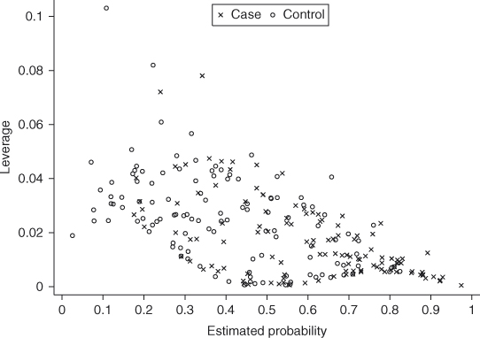
We plot the 238 estimated leverage values in Figure 7.1 using an “x” to indicate the case and an “o” to indicate a control. There are two controls and two cases with leverage values that fall well away from the rest of the plotted values. We remind the reader that leverage in a matched data setting is “distance from the weighted match set mean”. Once we have examined all the diagnostic statistics we present a table containing all identified observations and their data.
Figure 7.1 Plot of all 238 leverages versus the estimated probability from the fitted model from the GLOW ![]() Matched Study in Table 7.3.
Matched Study in Table 7.3.
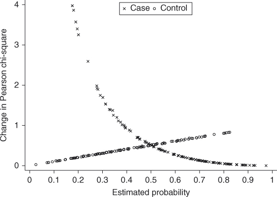
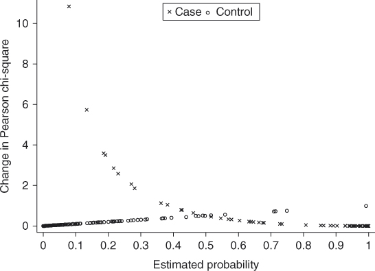
Next we examine the change in Pearson chi-square as a measure of lack of fit. We plot the 238 values in Figure 7.2. In the plot we see five values, all for cases, that are large relative to the other plotted values. In Chapter 5, we noted that we tend to define “large” as a value of ![]() . Here the five values are all between 3 and 4. Regardless, we still think it is important to identify any and all subjects with potentially extreme values and examine their effect on the fitted model.
. Here the five values are all between 3 and 4. Regardless, we still think it is important to identify any and all subjects with potentially extreme values and examine their effect on the fitted model.
Figure 7.2 Plot of all 238 values of ![]() versus the estimated probability from the fitted model from the GLOW
versus the estimated probability from the fitted model from the GLOW ![]() Matched Study in Table 7.3.
Matched Study in Table 7.3.
Next we examine the influence statistic ![]() with all 238 values plotted in Figure 7.3. We see two values that lie well away from the remainder of the plotted points and each one corresponds to a case.
with all 238 values plotted in Figure 7.3. We see two values that lie well away from the remainder of the plotted points and each one corresponds to a case.
Figure 7.3 Plot of all 238 values of ![]() versus the estimated probability from the fitted model from the GLOW
versus the estimated probability from the fitted model from the GLOW ![]() Matched Study in Table 7.3.
Matched Study in Table 7.3.

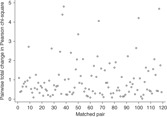
In the matched data setting we have two additional diagnostic statistics that estimate the effect of the matched set (pair here). These are the sum of the change in Pearson chi-square and influence over the subjects in each matched set. Here, we are interested in identifying the pair so plots are over the pair or matched set number rather than the estimated probability for one of the subjects in the matched set. The plot of the sum of the change in Pearson chi-square is shown in Figure 7.4 where we see 6 pairs with values that lie away from the other plotted values. Until we identify observations and pairs we cannot tell if these pairs correspond to the pairs whose individual cases were identified in any of the previous three plots.
Figure 7.4 Plot of pairwise sum of ![]() versus pair number from the fitted model from the GLOW
versus pair number from the fitted model from the GLOW ![]() Matched Study in Table 7.3.
Matched Study in Table 7.3.
We plot the pairwise sum of the Cook's distance diagnostic in Figure 7.5. We see only two values that seem to lie away from the rest of the plotted values. The next step is to identify subjects and pairs with extreme values in one or more of the figures.
Figure 7.5 Plot of pairwise sum of ![]() versus pair number from the fitted model from the GLOW
versus pair number from the fitted model from the GLOW ![]() Matched Study in Table 7.3.
Matched Study in Table 7.3.

Further examination of the values identified cases in pairs 37, 38, 67, 50, 100, and 117 as having a relatively large value of either or both ![]() and
and ![]() . These same pairs corresponded to large pairwise sum statistics in Figure 7.4 and/or Figure 7.5. Of the four pairs with large leverage values in Figure 7.1 only one, the case in pair 50, was identified in another plot. The data and diagnostic statistics from the case and the control in the six identified pairs are listed in Table 7.4.
. These same pairs corresponded to large pairwise sum statistics in Figure 7.4 and/or Figure 7.5. Of the four pairs with large leverage values in Figure 7.1 only one, the case in pair 50, was identified in another plot. The data and diagnostic statistics from the case and the control in the six identified pairs are listed in Table 7.4.
Table 7.4 Pair, Status, Covariates, and Diagnostic Statistics for Six Extreme Pairs

The first thing we notice in Table 7.4 is that the estimated probability of being the case is larger for the control than the case. There are 39 such pairs among the 119. When this occurs, it is not surprising that the summed measure of fit, sum ![]() , is large. The most influential of the six pairs is 50 with sum
, is large. The most influential of the six pairs is 50 with sum ![]() . In pair 50 the case weighs over 100 kg with a body mass index over 40 kg/m2 while the control weighs 57 kg with a body mass index of 22 kg/m2. Both sets of measurements are plausible, but with
. In pair 50 the case weighs over 100 kg with a body mass index over 40 kg/m2 while the control weighs 57 kg with a body mass index of 22 kg/m2. Both sets of measurements are plausible, but with ![]() the control looks more like a case than the case with
the control looks more like a case than the case with ![]() .
.
The next step is to examine the sensitivity of the fit to these six pairs. In the one to one matched design, if one deletes either the case or the control then the pair is deleted. One must have at least one value of each outcome in a pair for it to be included in the analysis. The values of the estimated coefficients and the percent change from those in Table 7.3 are given in Table 7.5.
Table 7.5 Estimated Coefficients from Table 7.3 (All), Estimated Coefficients when Pair Is Deleted, and Percent Change from All

When pairs are deleted one at a time none of the estimated coefficients change by more than 20 percent from the estimates when data from all 119 pairs are used. The largest change is −18 percent in the estimate of the coefficient for mother having had a fracture (MOMFRAC). Recall that when the percent change is negative it means that the estimate, with the pair removed, is larger than the estimate when the pair is included. The percent changes in the coefficients when all six pairs are removed are shown in the last line of Table 7.5. Here changes exceed 20 percent for each of the coefficients and, for MOMFRAC, it is a −46 percent change. The magnitude of these changes is not totally unexpected since, in all six pairs, the control had the larger estimated probability. So, in a sense, all six pairs go against the effects of the covariates in the fitted model and, when removed, their effects increase. While collectively the six pairs have a substantial impact on the magnitude of the estimates of the coefficients the actual values of the covariates are not at all unusual or extreme. Hence, we cannot, in good conscience, exclude them just because they happen to go against the model. Thus we proceed with the model in Table 7.3 as our final model.
The estimated odds ratio for each of the model covariates is given in Table 7.6, along with its 95 percent confidence interval. The results show that history of prior fracture, mother having had a fracture, and the need to use arms to rise from a chair each result in a more than twofold increase in the odds of fracture with the associated 95 percent confidence interval suggesting that the increase could be as little as a 1.2-fold or as much as a 4-fold increase for prior fracture and arm assist. Mother's history could be nonsignificant or result in as much as a 4.6-fold increase in the odds. There is an estimated 38 percent decrease in the odds of fracture for a 5 kg increase in weight and the decrease could be as small as 16 percent or as much as 54 percent with 95 percent confidence. Increasing body mass index by 5 kg/m2 is associated with a 3-fold in the odds of fracture and the increase in the odds could be as little as 1.4-fold or as much as 6.7-fold with 95 percent confidence.
Table 7.6 Estimated Odds Ratios and 95 Percent Confidence Intervals from the Fitted Model in Table 7.3
| Variable | Odds Ratio | 95% CI |
| Weight | 0.628 | 0.46, 0.84 |
| Body mass index | 3.049 | 1.38, 6.72 |
| History of prior fracture | 2.30 | 1.18, 4.48 |
| Mother had a fracture | 2.07 | 0.93, 4.61 |
| Need to use arms to rise from a chair | 2.43 | 1.18, 5.00 |
Odds ratio for a 5 kg increase in weight.
Odds ratio for a 5 kg/m2 increase in body mass index.
In summary, by following the purposeful selection method of main effects, factional polynomial analysis of continuous covariates and followed by purposeful selection of interactions, we obtained the relatively simple model shown in Table 7.3. One may also employ stepwise and best subsets selection of covariates described in Chapter 4 by obvious extensions of these methods. Extensions of the diagnostic statistics from Chapter 5 led us to identify six subjects that were either poorly fit or influential. The overall goodness of fit tests from Chapter 4 do not apply as the number of cases and controls are fixed by design. Clearly, once we account for the matching as a stratification variable and use conditional logistic regression, the modeling process proceeds as in the independent observation setting.
In closing this section, we note that many investigators break the matched pairs and proceed with the standard analysis as described in Chapters 4 and 5. Lynn and McCulloch (1992) provide some theoretical and simulation-based evidence for breaking the matches when the sample size is large. However, we believe that if data have been collected using a specific matched sampling design, then the analysis must have as its foundation the stratum-specific likelihood shown in equation 7.4 and the full likelihood in equation 7.3.
By ignoring the matching, we believe that investigators have used what is really an incorrect analysis for two basic reasons. First, the investigator probably is not comfortable with the conditional likelihood approach. He/she thinks that somehow the model has been changed and one cannot use estimated coefficients to estimate odds ratios in the usual manner. Second, until recently the analysis had to be performed using difference variables, a cumbersome and tedious data management task. We hope that the presentation of the example in this section convinces investigators that a matched analysis is no more difficult to carry out than an unmatched analysis.
7.4 An Example Using the Logistic Regression Model in a  Matched Study
The general approach to the analysis of the ![]() matched design and, for that matter, any general matched or highly stratified design, is quite similar to that of the
matched design and, for that matter, any general matched or highly stratified design, is quite similar to that of the ![]() matched design illustrated in the previous section. Again, we use STATA's clogit command, and associated diagnostic statistics to fit and analyze the model.
matched design illustrated in the previous section. Again, we use STATA's clogit command, and associated diagnostic statistics to fit and analyze the model.
In the ![]() matched design, the individual contribution of each matched pair to the likelihood in equation 7.4 is the conditional probability that the subject with
matched design, the individual contribution of each matched pair to the likelihood in equation 7.4 is the conditional probability that the subject with ![]() is the case among the two possible assignments of case status, the other being that the subject with
is the case among the two possible assignments of case status, the other being that the subject with ![]() is the case. In a
is the case. In a ![]() design, this same conditional probability is calculated (equation 7.4) but there are now
design, this same conditional probability is calculated (equation 7.4) but there are now ![]() possible assignments of case status to the matched subjects. Suppose, for example, that we consider a design where M = 3. Let the value of the covariates for the case in stratum
possible assignments of case status to the matched subjects. Suppose, for example, that we consider a design where M = 3. Let the value of the covariates for the case in stratum ![]() be denoted by
be denoted by ![]() and the values for the three controls be denoted
and the values for the three controls be denoted ![]() , and
, and ![]() . The contribution to the likelihood for this stratum of matched subjects from equation 7.4 is
. The contribution to the likelihood for this stratum of matched subjects from equation 7.4 is
The interpretation of equation 7.12, given the value of the coefficients, is the probability that the subject with data ![]() is the case relative to three controls with data
is the case relative to three controls with data ![]() , and
, and ![]() . We note that if the covariates are identical for all four subjects then the stratum is uninformative for estimation of the coefficients as
. We note that if the covariates are identical for all four subjects then the stratum is uninformative for estimation of the coefficients as ![]() for any value of
for any value of ![]() . For an individual covariate, there must be at least one control that has a value different from the case or the stratum is uninformative for that specific coefficient. Unfortunately, there are no simple expressions involving discordant pairs for the estimator of the coefficient for a dichotomous covariate in a univariable model. One statistic that is helpful in assessing the potential for “thin data” for a dichotomous covariate is identifying how many of the matched sets have the sum of the covariates over the
. For an individual covariate, there must be at least one control that has a value different from the case or the stratum is uninformative for that specific coefficient. Unfortunately, there are no simple expressions involving discordant pairs for the estimator of the coefficient for a dichotomous covariate in a univariable model. One statistic that is helpful in assessing the potential for “thin data” for a dichotomous covariate is identifying how many of the matched sets have the sum of the covariates over the ![]() subjects equal to 0 or
subjects equal to 0 or ![]() . As always, we feel it is good practice to fit univariable models and use the estimated standard errors and confidence intervals as indirect evaluation for “thin data”.
. As always, we feel it is good practice to fit univariable models and use the estimated standard errors and confidence intervals as indirect evaluation for “thin data”.
To provide a data set for an example and exercises we formed a ![]() matched data set from the Burn Study data described in Section 1.6.5 and Table 1.9. We used these data in Chapter 4 for one of the examples of model building. There we found that increasing age is an important risk factor in surviving a burn injury. In Chapter 4, we included age in the model. An alternative approach to estimating the effects of covariates controlling for age is to match cases (subjects who die), to controls (subjects who live) on age. Unlike the example in Section 7.3 using the GLOW Study data we could not match exactly on age. Instead we categorized age into 5-year intervals and matched each case with three randomly selected controls from the same age group. For some age groups it was not possible to identify three controls for the case identified. For these age groups we used only as many cases as could be matched. This resulted in 97 matched sets or strata. In practice we likely would have used
matched data set from the Burn Study data described in Section 1.6.5 and Table 1.9. We used these data in Chapter 4 for one of the examples of model building. There we found that increasing age is an important risk factor in surviving a burn injury. In Chapter 4, we included age in the model. An alternative approach to estimating the effects of covariates controlling for age is to match cases (subjects who die), to controls (subjects who live) on age. Unlike the example in Section 7.3 using the GLOW Study data we could not match exactly on age. Instead we categorized age into 5-year intervals and matched each case with three randomly selected controls from the same age group. For some age groups it was not possible to identify three controls for the case identified. For these age groups we used only as many cases as could be matched. This resulted in 97 matched sets or strata. In practice we likely would have used ![]() or
or ![]() matching in these age groups so as not to loose 28 cases. However, here the goal is to illustrate analyses with the conventional
matching in these age groups so as not to loose 28 cases. However, here the goal is to illustrate analyses with the conventional ![]() design. The covariates are listed in Table 1.9 and data are available at the web site as BURN13M and the covariate PAIR denotes the matched set.
design. The covariates are listed in Table 1.9 and data are available at the web site as BURN13M and the covariate PAIR denotes the matched set.
We found that each of the four dichotomous covariates, race (RACE), gender (GENDER), inhalation injury (INH_INJ), and flame involved (FLAME) had a number of strata where the covariate was constant. These are described in Table 7.7. We felt that for all four covariates there were a sufficient number of strata with a nonconstant sum to retain the covariate for analysis.
Table 7.7 Distributions of Strata with Constant Covariate Sum
| Covariate | Sum | Number of Strata |
| RACE | 0 | 3 |
| 4 | 10 | |
| GENDER | 0 | 3 |
| 4 | 25 | |
| INH_INJ | 0 | 26 |
| 4 | 0 | |
| FLAME | 0 | 1 |
| 4 | 17 |
Since there are only five covariates we began with a main effects model containing all five. The results of this fit are shown in Table 7.8. The Wald statistic ![]() -values suggest that GENDER and FLAME are not significant. Since the
-values suggest that GENDER and FLAME are not significant. Since the ![]() -value for FLAME is more than twice that of GENDER we next fit a model without FLAME. In results not shown, the likelihood ratio test comparing the model in Table 7.8 to one that excluded FLAME was not significant with
-value for FLAME is more than twice that of GENDER we next fit a model without FLAME. In results not shown, the likelihood ratio test comparing the model in Table 7.8 to one that excluded FLAME was not significant with ![]() . The Wald statistic for GENDER in the smaller model was not significant. We fit a model without GENDER and FLAME and confirmed that neither one contributed significantly to the model containing the remaining three covariates, nor was there any evidence of confounding. Hence our preliminary main effects model contains TBSA, RACE, and INH_INJ and is shown in Table 7.9.
. The Wald statistic for GENDER in the smaller model was not significant. We fit a model without GENDER and FLAME and confirmed that neither one contributed significantly to the model containing the remaining three covariates, nor was there any evidence of confounding. Hence our preliminary main effects model contains TBSA, RACE, and INH_INJ and is shown in Table 7.9.
Table 7.8 Estimated Coefficients, Estimated Standard Errors, Wald Statistics, and Two-Tailed ![]() -Values for the Multivariable Model Containing All Covariates
-Values for the Multivariable Model Containing All Covariates

Table 7.9 Estimated Coefficients, Estimated Standard Errors, Wald Statistics, and Two-Tailed ![]() -Values for the Preliminary Main Effects Model
-Values for the Preliminary Main Effects Model

The next step is to examine the scale of the continuous covariate total burn surface area (TBSA). In Chapter 4 using fractional polynomials we found that a model in ![]() was better than the linear model and not different from the best two term fractional polynomial model. However in this matched data set, fractional polynomial analysis using the closed test procedure did not yield a significant transformation. Further inspection of the results showed that the best one-term fractional polynomial model with power 0.5 did seem to offer some improvement over the linear model with
was better than the linear model and not different from the best two term fractional polynomial model. However in this matched data set, fractional polynomial analysis using the closed test procedure did not yield a significant transformation. Further inspection of the results showed that the best one-term fractional polynomial model with power 0.5 did seem to offer some improvement over the linear model with ![]() . However, the simplicity of the linear model and the fact that the preferred closed test procedure was not significant lead us to choose modeling TBSA as linear in the logit. We leave modeling using
. However, the simplicity of the linear model and the fact that the preferred closed test procedure was not significant lead us to choose modeling TBSA as linear in the logit. We leave modeling using ![]() as an exercise.
as an exercise.
For interactions among model covariates, we only examined the interaction of TBSA with INH_INJ as a burn surgeon felt there was no clinical basis for any interactions with RACE. This interaction was not significant with ![]() from the likelihood ratio test of the addition of the interaction to the model in Table 7.9. As noted in the previous section, the matching variable(s) can be effect modifiers, and thus it is good statistical practice to test for their interaction with model covariates. Rather than using the grouped age variable employed to create the matched case and three controls we used the actual value of age to form interactions with total burn surface area and inhalation injury. Neither interaction was significant at the five percent level. The AGE by TBSA interaction was significant at the 10 percent level. We leave as an exercise further analysis of a model with this interaction included. Hence, we continue using as our preliminary final model the one shown in Table 7.9.
from the likelihood ratio test of the addition of the interaction to the model in Table 7.9. As noted in the previous section, the matching variable(s) can be effect modifiers, and thus it is good statistical practice to test for their interaction with model covariates. Rather than using the grouped age variable employed to create the matched case and three controls we used the actual value of age to form interactions with total burn surface area and inhalation injury. Neither interaction was significant at the five percent level. The AGE by TBSA interaction was significant at the 10 percent level. We leave as an exercise further analysis of a model with this interaction included. Hence, we continue using as our preliminary final model the one shown in Table 7.9.
The next step is to obtain the values of the casewise and stratum sum diagnostic statistics presented in Section 7.2 and plot them versus a relevant quantity. The plot shown in Figure 7.6 is of the leverage from equation 7.7 versus the estimated stratum specific probability, ![]() . Recall that this probability estimates the stratum specific conditional probability that the subject is the case among the four subjects in the stratum. Hence, the sum of the four probabilities in each stratum is equal to one. In the figure, the controls are plotted using a small “o” and the cases are plotted using a small “x”. We see that three controls have leverage values that exceed 0.06 and fall somewhat away from the rest of the data. As in the non-matched setting, we see that the leverage goes to zero as the estimated probability approaches zero or one.
. Recall that this probability estimates the stratum specific conditional probability that the subject is the case among the four subjects in the stratum. Hence, the sum of the four probabilities in each stratum is equal to one. In the figure, the controls are plotted using a small “o” and the cases are plotted using a small “x”. We see that three controls have leverage values that exceed 0.06 and fall somewhat away from the rest of the data. As in the non-matched setting, we see that the leverage goes to zero as the estimated probability approaches zero or one.
Figure 7.6 Plot of all 338 leverage values versus the estimated probability from the fitted model from the BURN ![]() Matched Study in Table 7.9.
Matched Study in Table 7.9.

Next, we plot the values of the lack of fit diagnostic, ![]() , from equation 7.8 versus the estimated probability. In doing so, we found that two extremely large values of 134 and 54, belonging to cases, totally distorted the plot. Hence, we excluded these two cases and plotted the diagnostic statistic in Figure 7.7. Here we see that two cases have values exceeding 5 and lie away from the remainder of the data. So, in total, we found four cases with large values of the lack of fit diagnostic statistic.
, from equation 7.8 versus the estimated probability. In doing so, we found that two extremely large values of 134 and 54, belonging to cases, totally distorted the plot. Hence, we excluded these two cases and plotted the diagnostic statistic in Figure 7.7. Here we see that two cases have values exceeding 5 and lie away from the remainder of the data. So, in total, we found four cases with large values of the lack of fit diagnostic statistic.
Figure 7.7 Plot of 336 values of ![]() versus the estimated probability from the fitted model from the BURN
versus the estimated probability from the fitted model from the BURN ![]() Matched Study in Table 7.9.
Matched Study in Table 7.9.
The vales of the influence diagnostic statistic computed from equation 7.9 are plotted versus the estimated probability in Figure 7.8. The two values that lie well away from the rest of the data correspond to the two extremely poorly fit cases that we elected not to plot in Figure 7.7. No other values fall far enough from the rest of the data to cause concern.
Figure 7.8 Plot of all 338 values of ![]() versus the estimated probability from the fitted model from the BURN
versus the estimated probability from the fitted model from the BURN ![]() Matched Study in Table 7.9.
Matched Study in Table 7.9.

The plot of the sum of the four values of ![]() within 95 strata is shown in Figure 7.9. We excluded the two strata where the sum would exceed 50. The plot identifies the two strata containing the two cases identified in Figure 7.7.
within 95 strata is shown in Figure 7.9. We excluded the two strata where the sum would exceed 50. The plot identifies the two strata containing the two cases identified in Figure 7.7.
Figure 7.9 Plot of stratum sum of ![]() for values less than 50 versus stratum number from the fitted model from the BURN
for values less than 50 versus stratum number from the fitted model from the BURN ![]() Matched Study in Table 7.9.
Matched Study in Table 7.9.

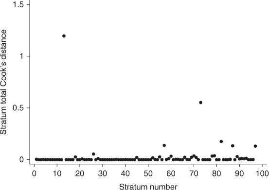
Next we plot, for all 97 strata, the sum of the four values of ![]() in Figure 7.10. The plot clearly identifies the two strata containing the cases that are poorly fit and excluded from Figure 7.9.
in Figure 7.10. The plot clearly identifies the two strata containing the cases that are poorly fit and excluded from Figure 7.9.
Figure 7.10 Plot of stratum sum of ![]() versus stratum number from the fitted model from the BURN
versus stratum number from the fitted model from the BURN ![]() Matched Study in Table 7.9.
Matched Study in Table 7.9.
Use of the diagnostic statistics identified three controls with high leverage. When we refit the model, in work not shown, excluding these three subjects, none of the estimated coefficients changed by more than 20 percent. Hence, we do not delete these controls and consider the poorly fit and/or influential cases.
The data and values of the diagnostic statistics are shown in Table 7.10. Stratum 13 is the most poorly fit and influential. The reason is that the case's data are more like a control, moderate burn size with an inhalation injury, and the first control's data are more like that of a case, quite large burn size and an inhalation injury. The same is true, but to a lesser extent, in stratum 73 where the case had only a two percent burn area while two of the controls had areas greater than 20 percent. For strata 82 and 87, the case is also poorly fit, but less so than strata 13 and 73, and the data for the cases look more like those for controls.
Table 7.10 Stratum, Status, Covariates, and Diagnostic Statistics for Stratum with the Largest Values of the Diagnostic Statistics
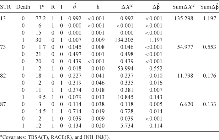
The next step is to sequentially delete each stratum, refit the model and compute the percent change in the coefficients from the estimates in Table 7.9. The results are shown in Table 7.11. When stratum 13 is deleted, the estimate of the coefficient for TBSA increases by 21 percent (see the definition of ![]() at the bottom of Table 7.11). When we delete stratum 73 the coefficient for RACE increases by 27.8 percent. No coefficient changes by more than 20 percent when either stratum 82 or stratum 87 is deleted. When all four strata are deleted, a total of 16 observations, each estimate increases by more than 40 percent. Hence the diagnostic statistics have identified influential cases. The question now is: Are the data for these subjects clinically implausible or did the subject just die or survive when the model would have predicted otherwise? The only subject whose result could be suspect is the first control in stratum 13. On further examination, we find that this subject is quite young, 21 years old, and while all subjects in this stratum are between 20 and 24 it is unusual to survive when 77 percent of the body is burned. In the end, the burn surgeon felt that none of the data are implausible and none should be excluded. Hence, we use the fitted model in Table 7.9 as our final model.
at the bottom of Table 7.11). When we delete stratum 73 the coefficient for RACE increases by 27.8 percent. No coefficient changes by more than 20 percent when either stratum 82 or stratum 87 is deleted. When all four strata are deleted, a total of 16 observations, each estimate increases by more than 40 percent. Hence the diagnostic statistics have identified influential cases. The question now is: Are the data for these subjects clinically implausible or did the subject just die or survive when the model would have predicted otherwise? The only subject whose result could be suspect is the first control in stratum 13. On further examination, we find that this subject is quite young, 21 years old, and while all subjects in this stratum are between 20 and 24 it is unusual to survive when 77 percent of the body is burned. In the end, the burn surgeon felt that none of the data are implausible and none should be excluded. Hence, we use the fitted model in Table 7.9 as our final model.
Table 7.11 Estimated Coefficients from Table 7.10 (All), Estimated Coefficients when Strata Are Deleted, and Percent Change from All

We explore in the exercises alternative modeling of these data that compares the matched analysis to an unmatched analysis.
The estimated odds ratios and corresponding 95 percent confidence intervals for the three covariates are given in Table 7.12. Under the assumption that the logit is linear in burn area we see that for every 10 percent increase in the size of the burn the odds of dying increases 3.5-fold and the increase could be as little as 2.2 or as much as 5.6 with 95 percent confidence. The model estimates that the odds of whites dying is 62 percent less than non-whites and is not significant at the five percent level but is at the 10 percent level. The confidence interval suggests that the decrease could be as much as 86 percent. Having an inhalation injury involved in the burn increases the odds of dying by almost 4-fold and could be as little as a 1.4-fold increase or as much as an 11-fold increase.
Table 7.12 Estimated Odds Ratios and 95 Percent Confidence Intervals from the Fitted Model in Table 7.9
| Variable | Odds Ratio | 95% CI |
| Total body surface area | 3.513 | 2.2, 5.6 |
| Race: whites verses non-whites13 | 0.38 | 0.14, 1.05 |
| Inhalation injury | 3.9 | 1.4, 11.0 |
Total burn surface area increase of 10%.
The data used for the example in this section does not contain as many covariates as might be available in practice. However, the analysis presented certainly provides a template that could be followed for modeling in more complicated data sets.
In summary, we have shown in this chapter that modeling in the matched case-control study follows the same methods as for unmatched studies discussed in previous chapters. In particular, the diagnostic statistics are highly useful in identifying subjects and strata that have high leverage, are poorly fit and/or influential. However, at this time, there are no overall goodness of fit tests of the type discussed in Section 5.2.
Exercises
1. Using the first control and the case in each of the 97 strata of the BURN ![]() matched data set, perform a complete
matched data set, perform a complete ![]() matched analysis.
matched analysis.
2. Repeat the analysis in Section 7.4 using the covariate ![]() in place of TBSA.
in place of TBSA.
3. Using the first and third controls and the case in each of the 97 strata of the Burn ![]() matched study, perform the analysis in this
matched study, perform the analysis in this ![]() matched data.
matched data.
4. Repeat the analysis in Section 7.4 as an unmatched case-control study including age as a covariate. Compare the results of this analysis to those in Section 7.4. Which analysis yields the more precise estimates of the odds ratios for TBSA, RACE, and INH_INJ?
5. Continue model building, evaluation, and presenting estimated odds ratios with the interaction between AGE and TBSA added to the model in Table 7.9.