
Chapter 1: Introduction to the Logistic Regression Model
1.1 Introduction
Regression methods have become an integral component of any data analysis concerned with describing the relationship between a response variable and one or more explanatory variables. Quite often the outcome variable is discrete, taking on two or more possible values. The logistic regression model is the most frequently used regression model for the analysis of these data.
Before beginning a thorough study of the logistic regression model it is important to understand that the goal of an analysis using this model is the same as that of any other regression model used in statistics, that is, to find the best fitting and most parsimonious, clinically interpretable model to describe the relationship between an outcome (dependent or response) variable and a set of independent (predictor or explanatory) variables. The independent variables are often called covariates. The most common example of modeling, and one assumed to be familiar to the readers of this text, is the usual linear regression model where the outcome variable is assumed to be continuous.
What distinguishes a logistic regression model from the linear regression model is that the outcome variable in logistic regression is binary or dichotomous. This difference between logistic and linear regression is reflected both in the form of the model and its assumptions. Once this difference is accounted for, the methods employed in an analysis using logistic regression follow, more or less, the same general principles used in linear regression. Thus, the techniques used in linear regression analysis motivate our approach to logistic regression. We illustrate both the similarities and differences between logistic regression and linear regression with an example.
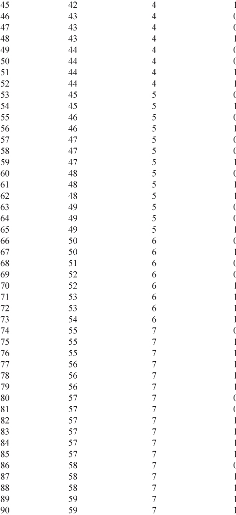
Example 1: Table 1.1 lists the age in years (AGE), and presence or absence of evidence of significant coronary heart disease (CHD) for 100 subjects in a hypothetical study of risk factors for heart disease. The table also contains an identifier variable (ID) and an age group variable (AGEGRP). The outcome variable is CHD, which is coded with a value of “0” to indicate that CHD is absent, or “1” to indicate that it is present in the individual. In general, any two values could be used, but we have found it most convenient to use zero and one. We refer to this data set as the CHDAGE data.
Table 1.1 Age, Age Group, and Coronary Heart Disease (CHD) Status of 100 Subjects


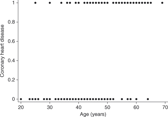
It is of interest to explore the relationship between AGE and the presence or absence of CHD in this group. Had our outcome variable been continuous rather than binary, we probably would begin by forming a scatterplot of the outcome versus the independent variable. We would use this scatterplot to provide an impression of the nature and strength of any relationship between the outcome and the independent variable. A scatterplot of the data in Table 1.1 is given in Figure 1.1.
Figure 1.1 Scatterplot of presence or absence of coronary heart disease (CHD) by AGE for 100 subjects.
In this scatterplot, all points fall on one of two parallel lines representing the absence of CHD (![]() ) or the presence of CHD (
) or the presence of CHD (![]() ). There is some tendency for the individuals with no evidence of CHD to be younger than those with evidence of CHD. While this plot does depict the dichotomous nature of the outcome variable quite clearly, it does not provide a clear picture of the nature of the relationship between CHD and AGE.
). There is some tendency for the individuals with no evidence of CHD to be younger than those with evidence of CHD. While this plot does depict the dichotomous nature of the outcome variable quite clearly, it does not provide a clear picture of the nature of the relationship between CHD and AGE.
The main problem with Figure 1.1 is that the variability in CHD at all ages is large. This makes it difficult to see any functional relationship between AGE and CHD. One common method of removing some variation, while still maintaining the structure of the relationship between the outcome and the independent variable, is to create intervals for the independent variable and compute the mean of the outcome variable within each group. We use this strategy by grouping age into the categories (AGEGRP) defined in Table 1.1. Table 1.2 contains, for each age group, the frequency of occurrence of each outcome, as well as the percent with CHD present.
Table 1.2 Frequency Table of Age Group by CHD

By examining this table, a clearer picture of the relationship begins to emerge. It shows that as age increases, the proportion (mean) of individuals with evidence of CHD increases. Figure 1.2 presents a plot of the percent of individuals with CHD versus the midpoint of each age interval. This plot provides considerable insight into the relationship between CHD and AGE in this study, but the functional form for this relationship needs to be described. The plot in this figure is similar to what one might obtain if this same process of grouping and averaging were performed in a linear regression. We note two important differences.
Figure 1.2 Plot of the percentage of subjects with CHD in each AGE group.

The first difference concerns the nature of the relationship between the outcome and independent variables. In any regression problem the key quantity is the mean value of the outcome variable, given the value of the independent variable. This quantity is called the conditional mean and is expressed as “![]() ” where
” where ![]() denotes the outcome variable and
denotes the outcome variable and ![]() denotes a specific value of the independent variable. The quantity
denotes a specific value of the independent variable. The quantity ![]() is read “the expected value of
is read “the expected value of ![]() , given the value
, given the value ![]() ”. In linear regression we assume that this mean may be expressed as an equation linear in
”. In linear regression we assume that this mean may be expressed as an equation linear in ![]() (or some transformation of
(or some transformation of ![]() or
or ![]() ), such as
), such as
![]()
This expression implies that it is possible for ![]() to take on any value as
to take on any value as ![]() ranges between
ranges between ![]() and
and ![]() .
.
The column labeled “Mean” in Table 1.2 provides an estimate of ![]() . We assume, for purposes of exposition, that the estimated values plotted in Figure 1.2 are close enough to the true values of
. We assume, for purposes of exposition, that the estimated values plotted in Figure 1.2 are close enough to the true values of ![]() to provide a reasonable assessment of the functional relationship between CHD and AGE. With a dichotomous outcome variable, the conditional mean must be greater than or equal to zero and less than or equal to one (i.e.,
to provide a reasonable assessment of the functional relationship between CHD and AGE. With a dichotomous outcome variable, the conditional mean must be greater than or equal to zero and less than or equal to one (i.e., ![]() ). This can be seen in Figure 1.2. In addition, the plot shows that this mean approaches zero and one “gradually”. The change in the
). This can be seen in Figure 1.2. In addition, the plot shows that this mean approaches zero and one “gradually”. The change in the ![]() per unit change in
per unit change in ![]() becomes progressively smaller as the conditional mean gets closer to zero or one. The curve is said to be S-shaped and resembles a plot of the cumulative distribution of a continuous random variable. Thus, it should not seem surprising that some well-known cumulative distributions have been used to provide a model for
becomes progressively smaller as the conditional mean gets closer to zero or one. The curve is said to be S-shaped and resembles a plot of the cumulative distribution of a continuous random variable. Thus, it should not seem surprising that some well-known cumulative distributions have been used to provide a model for ![]() in the case when
in the case when ![]() is dichotomous. The model we use is based on the logistic distribution.
is dichotomous. The model we use is based on the logistic distribution.
Many distribution functions have been proposed for use in the analysis of a dichotomous outcome variable. Cox and Snell (1989) discuss some of these. There are two primary reasons for choosing the logistic distribution. First, from a mathematical point of view, it is an extremely flexible and easily used function. Second, its model parameters provide the basis for clinically meaningful estimates of effect. A detailed discussion of the interpretation of the model parameters is given in Chapter 3.
In order to simplify notation, we use the quantity ![]() to represent the conditional mean of
to represent the conditional mean of ![]() given
given ![]() when the logistic distribution is used. The specific form of the logistic regression model we use is:
when the logistic distribution is used. The specific form of the logistic regression model we use is:
A transformation of ![]() that is central to our study of logistic regression is the logit transformation. This transformation is defined, in terms of
that is central to our study of logistic regression is the logit transformation. This transformation is defined, in terms of ![]() , as:
, as:

The importance of this transformation is that ![]() has many of the desirable properties of a linear regression model. The logit,
has many of the desirable properties of a linear regression model. The logit, ![]() , is linear in its parameters, may be continuous, and may range from
, is linear in its parameters, may be continuous, and may range from ![]() to
to ![]() , depending on the range of
, depending on the range of ![]() .
.
The second important difference between the linear and logistic regression models concerns the conditional distribution of the outcome variable. In the linear regression model we assume that an observation of the outcome variable may be expressed as ![]() . The quantity
. The quantity ![]() is called the error and expresses an observation's deviation from the conditional mean. The most common assumption is that
is called the error and expresses an observation's deviation from the conditional mean. The most common assumption is that ![]() follows a normal distribution with mean zero and some variance that is constant across levels of the independent variable. It follows that the conditional distribution of the outcome variable given
follows a normal distribution with mean zero and some variance that is constant across levels of the independent variable. It follows that the conditional distribution of the outcome variable given ![]() is normal with mean
is normal with mean ![]() , and a variance that is constant. This is not the case with a dichotomous outcome variable. In this situation, we may express the value of the outcome variable given
, and a variance that is constant. This is not the case with a dichotomous outcome variable. In this situation, we may express the value of the outcome variable given ![]() as
as ![]() . Here the quantity
. Here the quantity ![]() may assume one of two possible values. If
may assume one of two possible values. If ![]() then
then ![]() with probability
with probability ![]() , and if
, and if ![]() then
then ![]() with probability
with probability ![]() . Thus,
. Thus, ![]() has a distribution with mean zero and variance equal to
has a distribution with mean zero and variance equal to ![]() . That is, the conditional distribution of the outcome variable follows a binomial distribution with probability given by the conditional mean,
. That is, the conditional distribution of the outcome variable follows a binomial distribution with probability given by the conditional mean, ![]() .
.
In summary, we have shown that in a regression analysis when the outcome variable is dichotomous:
1.2 Fitting the Logistic Regression Model
Suppose we have a sample of n independent observations of the pair ![]()
![]() where
where ![]() denotes the value of a dichotomous outcome variable and
denotes the value of a dichotomous outcome variable and ![]() is the value of the independent variable for the
is the value of the independent variable for the ![]() subject. Furthermore, assume that the outcome variable has been coded as 0 or 1, representing the absence or the presence of the characteristic, respectively. This coding for a dichotomous outcome is used throughout the text. Fitting the logistic regression model in equation 1.1 to a set of data requires that we estimate the values of
subject. Furthermore, assume that the outcome variable has been coded as 0 or 1, representing the absence or the presence of the characteristic, respectively. This coding for a dichotomous outcome is used throughout the text. Fitting the logistic regression model in equation 1.1 to a set of data requires that we estimate the values of ![]() and
and ![]() , the unknown parameters.
, the unknown parameters.
In linear regression, the method used most often for estimating unknown parameters is least squares. In that method we choose those values of ![]() and
and ![]() that minimize the sum-of-squared deviations of the observed values of
that minimize the sum-of-squared deviations of the observed values of ![]() from the predicted values based on the model. Under the usual assumptions for linear regression the method of least squares yields estimators with a number of desirable statistical properties. Unfortunately, when the method of least squares is applied to a model with a dichotomous outcome, the estimators no longer have these same properties.
from the predicted values based on the model. Under the usual assumptions for linear regression the method of least squares yields estimators with a number of desirable statistical properties. Unfortunately, when the method of least squares is applied to a model with a dichotomous outcome, the estimators no longer have these same properties.
The general method of estimation that leads to the least squares function under the linear regression model (when the error terms are normally distributed) is called maximum likelihood. This method provides the foundation for our approach to estimation with the logistic regression model throughout this text. In a general sense, the method of maximum likelihood yields values for the unknown parameters that maximize the probability of obtaining the observed set of data. In order to apply this method we must first construct a function, called the likelihood function. This function expresses the probability of the observed data as a function of the unknown parameters. The maximum likelihood estimators of the parameters are the values that maximize this function. Thus, the resulting estimators are those that agree most closely with the observed data. We now describe how to find these values for the logistic regression model.
If ![]() is coded as 0 or 1 then the expression for
is coded as 0 or 1 then the expression for ![]() given in equation 1.1 provides (for an arbitrary value of
given in equation 1.1 provides (for an arbitrary value of ![]() , the vector of parameters) the conditional probability that
, the vector of parameters) the conditional probability that ![]() is equal to 1 given
is equal to 1 given ![]() . This is denoted as
. This is denoted as ![]() . It follows that the quantity
. It follows that the quantity ![]() gives the conditional probability that
gives the conditional probability that ![]() is equal to zero given
is equal to zero given ![]() ,
, ![]() . Thus, for those pairs
. Thus, for those pairs ![]() , where
, where ![]() , the contribution to the likelihood function is
, the contribution to the likelihood function is ![]() , and for those pairs where
, and for those pairs where ![]() , the contribution to the likelihood function is
, the contribution to the likelihood function is ![]() , where the quantity
, where the quantity ![]() denotes the value of
denotes the value of ![]() computed at
computed at ![]() . A convenient way to express the contribution to the likelihood function for the pair
. A convenient way to express the contribution to the likelihood function for the pair ![]() is through the expression
is through the expression
As the observations are assumed to be independent, the likelihood function is obtained as the product of the terms given in equation 1.2 as follows:

The principle of maximum likelihood states that we use as our estimate of ![]() the value that maximizes the expression in equation 1.3. However, it is easier mathematically to work with the log of equation 1.3. This expression, the log-likelihood, is defined as
the value that maximizes the expression in equation 1.3. However, it is easier mathematically to work with the log of equation 1.3. This expression, the log-likelihood, is defined as

To find the value of ![]() that maximizes
that maximizes ![]() we differentiate
we differentiate ![]() with respect to
with respect to ![]() and
and ![]() and set the resulting expressions equal to zero. These equations, known as the likelihood equations, are
and set the resulting expressions equal to zero. These equations, known as the likelihood equations, are
and
In equations 1.5 and 1.6 it is understood that the summation is over ![]() varying from 1 to
varying from 1 to ![]() . (The practice of suppressing the index and range of summation, when these are clear, is followed throughout this text.)
. (The practice of suppressing the index and range of summation, when these are clear, is followed throughout this text.)
In linear regression, the likelihood equations, obtained by differentiating the sum-of-squared deviations function with respect to ![]() are linear in the unknown parameters and thus are easily solved. For logistic regression the expressions in equations 1.5 and 1.6 are nonlinear in
are linear in the unknown parameters and thus are easily solved. For logistic regression the expressions in equations 1.5 and 1.6 are nonlinear in ![]() and
and ![]() , and thus require special methods for their solution. These methods are iterative in nature and have been programmed into logistic regression software. For the moment, we need not be concerned about these iterative methods and view them as a computational detail that is taken care of for us. The interested reader may consult the text by McCullagh and Nelder (1989) for a general discussion of the methods used by most programs. In particular, they show that the solution to equations 1.5 and 1.6 may be obtained using an iterative weighted least squares procedure.
, and thus require special methods for their solution. These methods are iterative in nature and have been programmed into logistic regression software. For the moment, we need not be concerned about these iterative methods and view them as a computational detail that is taken care of for us. The interested reader may consult the text by McCullagh and Nelder (1989) for a general discussion of the methods used by most programs. In particular, they show that the solution to equations 1.5 and 1.6 may be obtained using an iterative weighted least squares procedure.
The value of ![]() given by the solution to equations 1.5 and 1.6 is called the maximum likelihood estimate and is denoted as
given by the solution to equations 1.5 and 1.6 is called the maximum likelihood estimate and is denoted as ![]() . In general, the use of the symbol “
. In general, the use of the symbol “ ![]() ” denotes the maximum likelihood estimate of the respective quantity. For example,
” denotes the maximum likelihood estimate of the respective quantity. For example, ![]() is the maximum likelihood estimate of
is the maximum likelihood estimate of ![]() . This quantity provides an estimate of the conditional probability that
. This quantity provides an estimate of the conditional probability that ![]() is equal to 1, given that
is equal to 1, given that ![]() is equal to
is equal to ![]() . As such, it represents the fitted or predicted value for the logistic regression model. An interesting consequence of equation 1.5 is that
. As such, it represents the fitted or predicted value for the logistic regression model. An interesting consequence of equation 1.5 is that

That is, the sum of the observed values of ![]() is equal to the sum of the predicted (expected) values. We use this property in later chapters when we discuss assessing the fit of the model.
is equal to the sum of the predicted (expected) values. We use this property in later chapters when we discuss assessing the fit of the model.
As an example, consider the data given in Table 1.1. Use of a logistic regression software package, with continuous variable AGE as the independent variable, produces the output in Table 1.3.
Table 1.3 Results of Fitting the Logistic Regression Model to the CHDAGE Data, n = 100

The maximum likelihood estimates of ![]() and
and ![]() are
are ![]() and
and ![]() . The fitted values are given by the equation
. The fitted values are given by the equation
and the estimated logit, ![]() , is given by the equation
, is given by the equation
The log-likelihood given in Table 1.3 is the value of equation 1.4 computed using ![]() and
and ![]() .
.
Three additional columns are present in Table 1.3. One contains estimates of the standard errors of the estimated coefficients, the next column displays the ratios of the estimated coefficients to their estimated standard errors, and the last column displays a ![]() -value. These quantities are discussed in the next section.
-value. These quantities are discussed in the next section.
Following the fitting of the model we begin to evaluate its adequacy.
1.3 Testing for the Significance of the Coefficients
In practice, the modeling of a set of data, as we show in Chapters 4,7, and 8, is a much more complex process than one of simply fitting and testing. The methods we present in this section, while simplistic, do provide essential building blocks for the more complex process.
After estimating the coefficients, our first look at the fitted model commonly concerns an assessment of the significance of the variables in the model. This usually involves formulation and testing of a statistical hypothesis to determine whether the independent variables in the model are “significantly” related to the outcome variable. The method for performing this test is quite general, and differs from one type of model to the next only in the specific details. We begin by discussing the general approach for a single independent variable. The multivariable case is considered in Chapter 2.
One approach to testing for the significance of the coefficient of a variable in any model relates to the following question. Does the model that includes the variable in question tell us more about the outcome (or response) variable than a model that does not include that variable? This question is answered by comparing the observed values of the response variable to those predicted by each of two models; the first with, and the second without, the variable in question. The mathematical function used to compare the observed and predicted values depends on the particular problem. If the predicted values with the variable in the model are better, or more accurate in some sense, than when the variable is not in the model, then we feel that the variable in question is “significant”. It is important to note that we are not considering the question of whether the predicted values are an accurate representation of the observed values in an absolute sense (this is called goodness of fit). Instead, our question is posed in a relative sense. The assessment of goodness of fit is a more complex question that is discussed in detail in Chapter 5.
The general method for assessing significance of variables is easily illustrated in the linear regression model, and its use there motivates the approach used for logistic regression. A comparison of the two approaches highlights the differences between modeling continuous and dichotomous response variables.
In linear regression, one assesses the significance of the slope coefficient by forming what is referred to as an analysis of variance table. This table partitions the total sum-of-squared deviations of observations about their mean into two parts: (1) the sum-of-squared deviations of observations about the regression line SSE (or residual sum-of-squares) and (2) the sum-of-squares of predicted values, based on the regression model, about the mean of the dependent variable SSR (or due regression sum-of-squares). This is just a convenient way of displaying the comparison of observed to predicted values under two models. In linear regression, the comparison of observed and predicted values is based on the square of the distance between the two. If ![]() denotes the observed value and
denotes the observed value and ![]() denotes the predicted value for the ith individual under the model, then the statistic used to evaluate this comparison is
denotes the predicted value for the ith individual under the model, then the statistic used to evaluate this comparison is
Under the model not containing the independent variable in question the only parameter is ![]() , and
, and ![]() , the mean of the response variable. In this case,
, the mean of the response variable. In this case, ![]() and SSE is equal to the total sum-of-squares. When we include the independent variable in the model, any decrease in SSE is due to the fact that the slope coefficient for the independent variable is not zero. The change in the value of SSE is due to the regression source of variability, denoted SSR. That is,
and SSE is equal to the total sum-of-squares. When we include the independent variable in the model, any decrease in SSE is due to the fact that the slope coefficient for the independent variable is not zero. The change in the value of SSE is due to the regression source of variability, denoted SSR. That is,

In linear regression, interest focuses on the size of SSR. A large value suggests that the independent variable is important, whereas a small value suggests that the independent variable is not helpful in predicting the response.
The guiding principle with logistic regression is the same: compare observed values of the response variable to predicted values obtained from models, with and without the variable in question. In logistic regression, comparison of observed to predicted values is based on the log-likelihood function defined in equation 1.4. To better understand this comparison, it is helpful conceptually to think of an observed value of the response variable as also being a predicted value resulting from a saturated model. A saturated model is one that contains as many parameters as there are data points. (A simple example of a saturated model is fitting a linear regression model when there are only two data points, ![]() .)
.)
The comparison of observed to predicted values using the likelihood function is based on the following expression:
The quantity inside the large brackets in the expression above is called the likelihood ratio. Using minus twice its log is necessary to obtain a quantity whose distribution is known and can therefore be used for hypothesis testing purposes. Such a test is called the likelihood ratio test. Using equation 1.4, equation 1.9 becomes

where ![]() .
.
The statistic, ![]() , in equation 1.10 is called the deviance, and for logistic regression, it plays the same role that the residual sum-of-squares plays in linear regression. In fact, the deviance as shown in equation 1.10, when computed for linear regression, is identically equal to the SSE.
, in equation 1.10 is called the deviance, and for logistic regression, it plays the same role that the residual sum-of-squares plays in linear regression. In fact, the deviance as shown in equation 1.10, when computed for linear regression, is identically equal to the SSE.
Furthermore, in a setting as shown in Table 1.1, where the values of the outcome variable are either 0 or 1, the likelihood of the saturated model is identically equal to 1.0. Specifically, it follows from the definition of a saturated model that ![]() and the likelihood is
and the likelihood is

Thus it follows from equation 1.9 that the deviance is
Some software packages report the value of the deviance in equation 1.11 rather than the log-likelihood for the fitted model. In the context of testing for the significance of a fitted model, we want to emphasize that we think of the deviance in the same way that we think of the residual sum-of-squares in linear regression.
In particular, to assess the significance of an independent variable we compare the value of ![]() with and without the independent variable in the equation. The change in
with and without the independent variable in the equation. The change in ![]() due to the inclusion of the independent variable in the model is:
due to the inclusion of the independent variable in the model is:
![]()
This statistic, ![]() , plays the same role in logistic regression that the numerator of the partial
, plays the same role in logistic regression that the numerator of the partial ![]() -test does in linear regression. Because the likelihood of the saturated model is always common to both values of
-test does in linear regression. Because the likelihood of the saturated model is always common to both values of ![]() being differenced,
being differenced, ![]() can be expressed as
can be expressed as
1.12 ![]()
For the specific case of a single independent variable, it is easy to show that when the variable is not in the model, the maximum likelihood estimate of ![]() is
is ![]() where
where ![]() and
and ![]() and the predicted probability for all subjects is constant, and equal to
and the predicted probability for all subjects is constant, and equal to ![]() . In this setting, the value of
. In this setting, the value of ![]() is:
is:
1.13 
or

Under the hypothesis that ![]() is equal to zero, the statistic
is equal to zero, the statistic ![]() follows a chi-square distribution with 1 degree of freedom. Additional mathematical assumptions are needed; however, for the above case they are rather nonrestrictive, and involve having a sufficiently large sample size,
follows a chi-square distribution with 1 degree of freedom. Additional mathematical assumptions are needed; however, for the above case they are rather nonrestrictive, and involve having a sufficiently large sample size, ![]() , and enough subjects with both
, and enough subjects with both ![]() and
and ![]() . We discuss in later chapters that, as far as sample size is concerned, the key determinant is
. We discuss in later chapters that, as far as sample size is concerned, the key determinant is ![]() .
.
As an example, we consider the model fit to the data in Table 1.1, whose estimated coefficients and log-likelihood are given in Table 1.3. For these data the sample size is sufficiently large as ![]() and
and ![]() . Evaluating
. Evaluating ![]() as shown in equation 1.14 yields
as shown in equation 1.14 yields
![]()
The first term in this expression is the log-likelihood from the model containing age (see Table 1.3), and the remainder of the expression simply substitutes ![]() and
and ![]() into the second part of equation 1.14. We use the symbol
into the second part of equation 1.14. We use the symbol ![]() to denote a chi-square random variable with
to denote a chi-square random variable with ![]() degrees of freedom. Using this notation, the
degrees of freedom. Using this notation, the ![]() -value associated with this test is
-value associated with this test is ![]() ; thus, we have convincing evidence that AGE is a significant variable in predicting CHD. This is merely a statement of the statistical evidence for this variable. Other important factors to consider before concluding that the variable is clinically important would include the appropriateness of the fitted model, as well as inclusion of other potentially important variables.
; thus, we have convincing evidence that AGE is a significant variable in predicting CHD. This is merely a statement of the statistical evidence for this variable. Other important factors to consider before concluding that the variable is clinically important would include the appropriateness of the fitted model, as well as inclusion of other potentially important variables.
As all logistic regression software report either the value of the log-likelihood or the value of ![]() , it is easy to check for the significance of the addition of new terms to the model or to verify a reported value of
, it is easy to check for the significance of the addition of new terms to the model or to verify a reported value of ![]() . In the simple case of a single independent variable, we first fit a model containing only the constant term. Next, we fit a model containing the independent variable along with the constant. This gives rise to another log-likelihood. The likelihood ratio test is obtained by multiplying the difference between these two values by
. In the simple case of a single independent variable, we first fit a model containing only the constant term. Next, we fit a model containing the independent variable along with the constant. This gives rise to another log-likelihood. The likelihood ratio test is obtained by multiplying the difference between these two values by ![]() .
.
In the current example, the log-likelihood for the model containing only a constant term is ![]() . Fitting a model containing the independent variable (AGE) along with the constant term results in the log-likelihood shown in Table 1.3 of
. Fitting a model containing the independent variable (AGE) along with the constant term results in the log-likelihood shown in Table 1.3 of ![]() . Multiplying the difference in these log-likelihoods by
. Multiplying the difference in these log-likelihoods by ![]() gives
gives
![]()
This result, along with the associated ![]() -value for the chi-square distribution, is commonly reported in logistic regression software packages.
-value for the chi-square distribution, is commonly reported in logistic regression software packages.
There are two other statistically equivalent tests: the Wald test and the Score test. The assumptions needed for each of these is the same as those of the likelihood ratio test in equation 1.14. A more complete discussion of these three tests and their assumptions may be found in Rao (1973).
The Wald test is equal to the ratio of the maximum likelihood estimate of the slope parameter, ![]() , to an estimate of its standard error. Under the null hypothesis and the sample size assumptions, this ratio follows a standard normal distribution. While we have not yet formally discussed how the estimates of the standard errors of the estimated parameters are obtained, they are routinely printed out by computer software. For example, the Wald test for the coefficient for AGE in Table 1.3 is provided in the column headed
, to an estimate of its standard error. Under the null hypothesis and the sample size assumptions, this ratio follows a standard normal distribution. While we have not yet formally discussed how the estimates of the standard errors of the estimated parameters are obtained, they are routinely printed out by computer software. For example, the Wald test for the coefficient for AGE in Table 1.3 is provided in the column headed ![]() and is
and is

The two-tailed ![]() -value, provided in the last column of Table 1.3, is
-value, provided in the last column of Table 1.3, is ![]() , where
, where ![]() denotes a random variable following the standard normal distribution. Some software packages display the statistic
denotes a random variable following the standard normal distribution. Some software packages display the statistic ![]() , which is distributed as chi-square with 1 degree of freedom. Hauck and Donner (1977) examined the performance of the Wald test and found that it behaved in an aberrant manner, often failing to reject the null hypothesis when the coefficient was significant using the likelihood ratio test. Thus, they recommended (and we agree) that the likelihood ratio test is preferred. We note that while the assertions of Hauk and Donner are true, we have never seen huge differences in the values of
, which is distributed as chi-square with 1 degree of freedom. Hauck and Donner (1977) examined the performance of the Wald test and found that it behaved in an aberrant manner, often failing to reject the null hypothesis when the coefficient was significant using the likelihood ratio test. Thus, they recommended (and we agree) that the likelihood ratio test is preferred. We note that while the assertions of Hauk and Donner are true, we have never seen huge differences in the values of ![]() and
and ![]() . In practice, the more troubling situation is when the values are close, and one test has
. In practice, the more troubling situation is when the values are close, and one test has ![]() and the other has
and the other has ![]() When this occurs, we use the
When this occurs, we use the ![]() -value from the likelihood ratio test.
-value from the likelihood ratio test.
A test for the significance of a variable that does not require computing the estimate of the coefficient is the score test. Proponents of the score test cite this reduced computational effort as its major advantage. Use of the test is limited by the fact that it is not available in many software packages. The score test is based on the distribution theory of the derivatives of the log-likelihood. In general, this is a multivariate test requiring matrix calculations that are discussed in Chapter 2.
In the univariate case, this test is based on the conditional distribution of the derivative in equation 1.6, given the derivative in equation 1.5. In this case, we can write down an expression for the Score test. The test uses the value of equation 1.6 computed using ![]() and
and ![]() . As noted earlier, under these parameter values,
. As noted earlier, under these parameter values, ![]() and the left-hand side of equation 1.6 becomes
and the left-hand side of equation 1.6 becomes ![]() . It may be shown that the estimated variance is
. It may be shown that the estimated variance is ![]() . The test statistic for the score test (ST) is
. The test statistic for the score test (ST) is
As an example of the score test, consider the model fit to the data in Table 1.1. The value of the test statistic for this example is
![]()
and the two tailed ![]() -value is
-value is ![]() . We note that, for this example, the values of the three test statistics are nearly the same (note:
. We note that, for this example, the values of the three test statistics are nearly the same (note: ![]() ).
).
In summary, the method for testing the significance of the coefficient of a variable in logistic regression is similar to the approach used in linear regression; however, it is based on the likelihood function for a dichotomous outcome variable under the logistic regression model.
1.4 Confidence Interval Estimation
An important adjunct to testing for significance of the model, discussed in Section 1.3, is calculation and interpretation of confidence intervals for parameters of interest. As is the case in linear regression we can obtain these for the slope, intercept and the “line” (i.e., the logit). In some settings it may be of interest to provide interval estimates for the fitted values (i.e., the predicted probabilities).
The basis for construction of the interval estimators is the same statistical theory we used to formulate the tests for significance of the model. In particular, the confidence interval estimators for the slope and intercept are, most often, based on their respective Wald tests and are sometimes referred to as Wald-based confidence intervals. The endpoints of a ![]() confidence interval for the slope coefficient are
confidence interval for the slope coefficient are
and for the intercept they are
where ![]() is the upper
is the upper ![]() point from the standard normal distribution and
point from the standard normal distribution and ![]() denotes a model-based estimator of the standard error of the respective parameter estimator. We defer discussion of the actual formula used for calculating the estimators of the standard errors to Chapter 2. For the moment, we use the fact that estimated values are provided in the output following the fit of a model and, in addition, many packages also provide the endpoints of the interval estimates.
denotes a model-based estimator of the standard error of the respective parameter estimator. We defer discussion of the actual formula used for calculating the estimators of the standard errors to Chapter 2. For the moment, we use the fact that estimated values are provided in the output following the fit of a model and, in addition, many packages also provide the endpoints of the interval estimates.
As an example, consider the model fit to the data in Table 1.1 regressing AGE on the presence or absence of CHD. The results are presented in Table 1.3. The endpoints of a 95 percent confidence interval for the slope coefficient from equation 1.15 are ![]() , yielding the interval
, yielding the interval ![]() . We defer a detailed discussion of the interpretation of these results to Chapter 3. Briefly, the results suggest that the change in the log-odds of CHD per one year increase in age is 0.111 and the change could be as little as 0.064 or as much as 0.158 with 95 percent confidence.
. We defer a detailed discussion of the interpretation of these results to Chapter 3. Briefly, the results suggest that the change in the log-odds of CHD per one year increase in age is 0.111 and the change could be as little as 0.064 or as much as 0.158 with 95 percent confidence.
As is the case with any regression model, the constant term provides an estimate of the response at ![]() unless the independent variable has been centered at some clinically meaningful value. In our example, the constant provides an estimate of the log-odds ratio of CHD at zero years of age. As a result, the constant term, by itself, has no useful clinical interpretation. In any event, from equation 1.16, the endpoints of a 95 percent confidence interval for the constant are
unless the independent variable has been centered at some clinically meaningful value. In our example, the constant provides an estimate of the log-odds ratio of CHD at zero years of age. As a result, the constant term, by itself, has no useful clinical interpretation. In any event, from equation 1.16, the endpoints of a 95 percent confidence interval for the constant are ![]() , yielding the interval
, yielding the interval ![]() .
.
The logit is the linear part of the logistic regression model and, as such, is most similar to the fitted line in a linear regression model. The estimator of the logit is
1.17 ![]()
The estimator of the variance of the estimator of the logit requires obtaining the variance of a sum. In this case it is
In general, the variance of a sum is equal to the sum of the variance of each term and twice the covariance of each possible pair of terms formed from the components of the sum. The endpoints of a ![]() Wald-based confidence interval for the logit are
Wald-based confidence interval for the logit are
1.19 ![]()
where ![]() is the positive square root of the variance estimator in equation 1.18.
is the positive square root of the variance estimator in equation 1.18.
The estimated logit for the fitted model in Table 1.3 is shown in equation 1.8. In order to evaluate equation 1.18 for a specific age we need the estimated covariance matrix. This matrix can be obtained from the output from all logistic regression software packages. How it is displayed varies from package to package, but the triangular form shown in Table 1.4 is a common one.
Table 1.4 Estimated Covariance Matrix of the Estimated Coefficients in Table 1.3
| Age | Constant | |
| Age | 0.000579 | |
| Constant | 1.28517 |
The estimated logit from equation 1.8 for a subject of age 50 is
![]()
the estimated variance, using equation 1.18 and the results in Table 1.4, is
![]()
and the estimated standard error is ![]() . Thus the end points of a 95 percent confidence interval for the logit at age 50 are
. Thus the end points of a 95 percent confidence interval for the logit at age 50 are
![]()
We discuss the interpretation and use of the estimated logit in providing estimates of odds ratios in Chapter 3.
The estimator of the logit and its confidence interval provide the basis for the estimator of the fitted value, in this case the logistic probability, and its associated confidence interval. In particular, using equation 1.7 at age 50 the estimated logistic probability is
and the endpoints of a 95 percent confidence interval are obtained from the respective endpoints of the confidence interval for the logit. The endpoints of the ![]() Wald-based confidence interval for the fitted value are
Wald-based confidence interval for the fitted value are
1.21 
Using the example at age 50 to demonstrate the calculations, the lower limit is
![]()
and the upper limit is
![]()
We have found that a major mistake often made by data analysts new to logistic regression modeling is to try and apply estimates on the probability scale to individual subjects. The fitted value computed in equation 1.20 is analogous to a particular point on the line obtained from a linear regression. In linear regression each point on the fitted line provides an estimate of the mean of the dependent variable in a population of subjects with covariate value “![]() ”. Thus the value of 0.56 in equation 1.20 is an estimate of the mean (i.e., proportion) of 50-year-old subjects in the population sampled that have evidence of CHD. An individual 50-year-old subject either does or does not have evidence of CHD. The confidence interval suggests that this mean could be between 0.435 and 0.677 with 95 percent confidence. We discuss the use and interpretation of fitted values in greater detail in Chapter 3.
”. Thus the value of 0.56 in equation 1.20 is an estimate of the mean (i.e., proportion) of 50-year-old subjects in the population sampled that have evidence of CHD. An individual 50-year-old subject either does or does not have evidence of CHD. The confidence interval suggests that this mean could be between 0.435 and 0.677 with 95 percent confidence. We discuss the use and interpretation of fitted values in greater detail in Chapter 3.
One application of fitted logistic regression models that has received a lot of attention in the subject matter literature is using model-based fitted values similar to the one in equation 1.20 to predict the value of a binary dependent value in individual subjects. This process is called classification and has a long history in statistics where it is referred to as discriminant analysis. We discuss the classification problem in detail in Chapter 4. We also discuss discriminant analysis within the context of a method for obtaining estimators of the coefficients in the next section.
The coverage12 of the Wald-based confidence interval estimators in equations 1.15 and 1.16 depends on the assumption that the distribution of the maximum likelihood estimators is normal. Potential sensitivity to this assumption is the main reason that the likelihood ratio test is recommended over the Wald test for assessing the significance of individual coefficients, as well as for the overall model. In settings where the number of events ![]() and/or the sample size is small the normality assumption is suspect and a log-likelihood function-based confidence interval can have better coverage. Until recently routines to compute these intervals were not available in most software packages. Cox and Snell (1989, p. 179–183) discuss the theory behind likelihood intervals, and Venzon and Moolgavkar (1988) describe an efficient way to calculate the end points. Royston (2007) describes a STATA [StataCorp (2011)] routine that implements the Venzon and Moolgavkar method that we use for the examples in this text. The SAS package's logistic regression procedure [SAS Institute Inc. (2009)] has the option to obtain likelihood confidence intervals.
and/or the sample size is small the normality assumption is suspect and a log-likelihood function-based confidence interval can have better coverage. Until recently routines to compute these intervals were not available in most software packages. Cox and Snell (1989, p. 179–183) discuss the theory behind likelihood intervals, and Venzon and Moolgavkar (1988) describe an efficient way to calculate the end points. Royston (2007) describes a STATA [StataCorp (2011)] routine that implements the Venzon and Moolgavkar method that we use for the examples in this text. The SAS package's logistic regression procedure [SAS Institute Inc. (2009)] has the option to obtain likelihood confidence intervals.
The likelihood-based confidence interval estimator for a coefficient can be concisely described as the interval of values, ![]() , for which the likelihood ratio test would fail to reject the hypothesis,
, for which the likelihood ratio test would fail to reject the hypothesis, ![]() , at the stated
, at the stated ![]() percent significance level. The two end points,
percent significance level. The two end points, ![]() and
and ![]() , of this interval for a coefficient are defined as follows:
, of this interval for a coefficient are defined as follows:
where ![]() is the value of the log-likelihood of the fitted model and
is the value of the log-likelihood of the fitted model and ![]() is the value of the profile log-likelihood. A value of the profile log-likelihood is computed by first specifying/fixing a value for the coefficient of interest, for example the slope coefficient for age, and then finding the value of the intercept coefficient, using the Venzon and Moolgavkar method, that maximizes the log-likelihood. This process is repeated over a grid of values of the specified coefficient, for example, values of
is the value of the profile log-likelihood. A value of the profile log-likelihood is computed by first specifying/fixing a value for the coefficient of interest, for example the slope coefficient for age, and then finding the value of the intercept coefficient, using the Venzon and Moolgavkar method, that maximizes the log-likelihood. This process is repeated over a grid of values of the specified coefficient, for example, values of ![]() , until the solutions to equation 1.22 are found. The results can be presented graphically or in standard interval form. We illustrate both in the example below.
, until the solutions to equation 1.22 are found. The results can be presented graphically or in standard interval form. We illustrate both in the example below.
As an example, we show in Figure 1.3 a plot of the profile log-likelihood for the coefficient for AGE using the CHDAGE data in Table 1.1. The end points of the 95 percent likelihood interval are ![]() and
and ![]() and are shown in the figure where the two vertical lines intersect the “
and are shown in the figure where the two vertical lines intersect the “![]() ” axis. The horizontal line in the figure is drawn at the value
” axis. The horizontal line in the figure is drawn at the value
![]()
where ![]() is the value of the log-likelihood of the fitted model from Table 1.3 and 3.8416 is the 95th percentile of the chi-square distribution with 1 degree of freedom.
is the value of the log-likelihood of the fitted model from Table 1.3 and 3.8416 is the 95th percentile of the chi-square distribution with 1 degree of freedom.
Figure 1.3 Plot of the profile log-likelihood for the coefficient for AGE in the CHDAGE data.
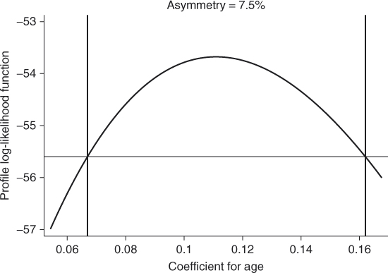
The quantity “Asymmetry” in Figure 1.3 is a measure of asymmetry of the profile log-likelihood that is the difference between the lengths of the upper part of the interval, ![]() , to the lower part,
, to the lower part, ![]() , as a percent of the total length,
, as a percent of the total length, ![]() . In the example the value is
. In the example the value is
![]()
As the upper and lower endpoints of the Wald-based confidence interval in equation 1.15 are equidistant from the maximum likelihood estimator, it has asymmetry ![]() .
.
In this example, the Wald-based confidence interval for the coefficient for age is ![]() . The likelihood interval is
. The likelihood interval is ![]() , which is only 1.1% wider than the Wald-based interval. So there is not a great deal of pure numeric difference in the two intervals and the asymmetry is small. In settings where there is greater asymmetry in the likelihood-based interval there can be more substantial differences between the two intervals. We return to this point in Chapter 3 where we discuss the interpretation of estimated coefficients. In addition, we include an exercise at the end of this chapter where there is a pronounced difference between the Wald and likelihood confidence interval estimators.
, which is only 1.1% wider than the Wald-based interval. So there is not a great deal of pure numeric difference in the two intervals and the asymmetry is small. In settings where there is greater asymmetry in the likelihood-based interval there can be more substantial differences between the two intervals. We return to this point in Chapter 3 where we discuss the interpretation of estimated coefficients. In addition, we include an exercise at the end of this chapter where there is a pronounced difference between the Wald and likelihood confidence interval estimators.
Methods to extend the likelihood intervals to functions of more than one coefficient such as the estimated logit function and probability are not available in current software packages.
1.5 Other Estimation Methods
The method of maximum likelihood described in Section 1.2 is the estimation method used in the logistic regression routines of the major software packages. However, two other methods have been and may still be used for estimating the coefficients. These methods are: (1) noniterative weighted least squares, and (2) discriminant function analysis.
A linear models approach to the analysis of categorical data proposed by Grizzle et al. (1969) [Grizzle, Starmer, and Koch (GSK) method] uses estimators based on noniterative weighted least squares. They demonstrate that the logistic regression model is an example of a general class of models that can be handled by their methods. We should add that the maximum likelihood estimators are usually calculated using an iterative reweighted least squares algorithm, and are also technically “least squares” estimators. The GSK method requires one iteration and is used in SAS's GENMOD procedure to fit a logistic regression model containing only categorical covariates.
A major limitation of the GSK method is that we must have an estimate of ![]() that is not zero or 1 for most values of
that is not zero or 1 for most values of ![]() . An example where we could use both maximum likelihood and GSK's noniterative weighted least squares is the data in Table 1.2. In cases such as this, the two methods are asymptotically equivalent, meaning that as
. An example where we could use both maximum likelihood and GSK's noniterative weighted least squares is the data in Table 1.2. In cases such as this, the two methods are asymptotically equivalent, meaning that as ![]() gets large, the distributional properties of the two estimators become identical. The GSK method could not be used with the data in Table 1.1.
gets large, the distributional properties of the two estimators become identical. The GSK method could not be used with the data in Table 1.1.
The discriminant function approach to estimation of the coefficients is of historical importance as it was popularized by Cornfield (1962) in some of the earliest work on logistic regression. These estimators take their name from the fact that the posterior probability in the usual discriminant function model is the logistic regression function given in equation 1.1. More precisely, if the independent variable, ![]() , follows a normal distribution within each of two groups (subpopulations) defined by the two values of
, follows a normal distribution within each of two groups (subpopulations) defined by the two values of ![]() and has different means and the same variance, then the conditional distribution of
and has different means and the same variance, then the conditional distribution of ![]() given
given ![]() is the logistic regression model. That is, if
is the logistic regression model. That is, if
![]()
then ![]() . The symbol “
. The symbol “![]() ” is read “is distributed” and the “
” is read “is distributed” and the “![]() ” denotes the normal distribution with mean equal to
” denotes the normal distribution with mean equal to ![]() and variance equal to
and variance equal to ![]() . Under these assumptions it is easy to show [Lachenbruch (1975)] that the logistic coefficients are
. Under these assumptions it is easy to show [Lachenbruch (1975)] that the logistic coefficients are
and
where ![]() The discriminant function estimators of
The discriminant function estimators of ![]() and
and ![]() are obtained by substituting estimators for
are obtained by substituting estimators for ![]() and
and ![]() into the above equations. The estimators usually used are
into the above equations. The estimators usually used are ![]() , the mean of
, the mean of ![]() in the subgroup defined by
in the subgroup defined by ![]() the mean of
the mean of ![]() with
with ![]() and
and
![]()
where ![]() is the unbiased estimator of
is the unbiased estimator of ![]() computed within the subgroup of the data defined by
computed within the subgroup of the data defined by ![]() . The above expressions are for a single variable
. The above expressions are for a single variable ![]() and multivariable expressions are presented in Chapter 2.
and multivariable expressions are presented in Chapter 2.
It is natural to ask why, if the discriminant function estimators are so easy to compute, they are not used in place of the maximum likelihood estimators? Halpern et al. (1971) and Hosmer et al. (1983) compared the two methods when the model contains a mixture of continuous and discrete variables, with the general conclusion that the discriminant function estimators are sensitive to the assumption of normality. In particular, the estimators of the coefficients for non-normally distributed variables are biased away from zero when the coefficient is, in fact, different from zero. The practical implication of this is that for dichotomous independent variables (that occur in many situations), the discriminant function estimators overestimate the magnitude of the coefficient. Lyles et al. (2009) describe a clever linear regression-based approach to compute the discriminant function estimator of the coefficient for a single continuous variable that, when their assumptions of normality hold, has better statistical properties than the maximum likelihood estimator. We discuss their multivariable extension and some of its practical limitations in Chapter 2.
At this point it may be helpful to delineate more carefully the various uses of the term maximum likelihood, as it applies to the estimation of the logistic regression coefficients. Under the assumptions of the discriminant function model stated above, the estimators obtained from equations 1.23 and 1.24 are maximum likelihood estimators. The estimators obtained from equations 1.5 and 1.6 are based on the conditional distribution of ![]() given
given ![]() and, as such, are technically “conditional maximum likelihood estimators”. It is common practice to drop the word “conditional” when describing the estimators given in equations 1.5 and 1.6. In this text, we use the word conditional to describe estimators in logistic regression with matched data as discussed in Chapter 7.
and, as such, are technically “conditional maximum likelihood estimators”. It is common practice to drop the word “conditional” when describing the estimators given in equations 1.5 and 1.6. In this text, we use the word conditional to describe estimators in logistic regression with matched data as discussed in Chapter 7.
In summary there are alternative methods of estimation for some data configurations that are computationally quicker; however, we use the maximum likelihood method described in Section 1.2 throughout the rest of this text.
1.6 Data Sets Used in Examples and Exercises
A number of different data sets are used in the examples as well as the exercises for the purpose of demonstrating various aspects of logistic regression modeling. Six of the data sets used throughout the text are described below. Other data sets are introduced as needed in later chapters. Some of the data sets were used in the previous editions of this text, for example the ICU and Low Birth Weight data, while others are new to this edition. All data sets used in this text may be obtained from links to web sites at John Wiley & Sons Inc. and the University of Massachusetts given in the Preface.
1.6.1 The ICU Study
The ICU study data set consists of a sample of 200 subjects who were part of a much larger study on survival of patients following admission to an adult intensive care unit (ICU). The major goal of this study was to develop a logistic regression model to predict the probability of survival to hospital discharge of these patients. A number of publications have appeared that have focused on various facets of this problem. The reader wishing to learn more about the clinical aspects of this study should start with Lemeshow et al. (1988). For a more up-to-date discussion of modeling the outcome of ICU patients the reader is referred to Lemeshow and Le Gall (1994) and to Lemeshow et al. (1993). The actual observed variable values have been modified to protect subject confidentiality. A code sheet for the variables to be considered in this text is given in Table 1.5. We refer to this data set as the ICU data.
Table 1.5 Code Sheet for the Variables in the ICU Data

1.6.2 The Low Birth Weight Study
Low birth weight, defined as birth weight less than 2500 grams, is an outcome that has been of concern to physicians for years. This is because of the fact that infant mortality rates and birth defect rates are higher for low birth weight babies. A woman's behavior during pregnancy (including diet, smoking habits, and receiving prenatal care) can greatly alter the chances of carrying the baby to term, and, consequently, of delivering a baby of normal birth weight.
Data were collected as part of a larger study at Baystate Medical Center in Springfield, Massachusetts. This data set contains information on 189 births to women seen in the obstetrics clinic. Fifty-nine of these births were low birth weight. The variables identified in the code sheet given in Table 1.6 have been shown to be associated with low birth weight in the obstetrical literature. The goal of the current study was to determine whether these variables were risk factors in the clinic population being served by Baystate Medical Center. Actual observed variable values have been modified to protect subject confidentiality. We refer to this data set as the LOWBWT data.
Table 1.6 Code Sheet for the Variables in the Low Birth Weight Data

1.6.3 The Global Longitudinal Study of Osteoporosis in Women
The Global Longitudinal Study of Osteoporosis in Women (GLOW) is an international study of osteoporosis in women over 55 years of age being coordinated at the Center for Outcomes Research (COR) at the University of Massachusetts/Worcester by its Director, Dr. Frederick Anderson, Jr. The study has enrolled over 60,000 women aged 55 and older in ten countries. The major goals of the study are to use the data to provide insights into the management of fracture risk, patient experience with prevention and treatment of fractures and distribution of risk factors among older women on an international scale over the follow up period. Complete details on the study as well as a list of GLOW publications may be found at the Center for Outcomes Research web site, www.outcomes-umassmed.org/glow.
Data used here come from six sites in the United States and include a few selected potential risk factors for fracture from the baseline questionnaire. The outcome variable is any fracture in the first year of follow up. The incident first-year fracture rate among the 21,000 subjects enrolled in these six sites is about 4 percent. In order to have a data set of a manageable size, ![]() , for this text we have over sampled the fractures and under sampled the non-fractures. As a result associations and conclusions from modeling these data do not apply to the study cohort as a whole. Data have been modified to protect subject confidentiality. We thank Dr. Gordon Fitzgerald of COR for his help in obtaining these data sets. A code sheet for the variables is shown in Table 1.7. This data set is named the GLOW500 data.
, for this text we have over sampled the fractures and under sampled the non-fractures. As a result associations and conclusions from modeling these data do not apply to the study cohort as a whole. Data have been modified to protect subject confidentiality. We thank Dr. Gordon Fitzgerald of COR for his help in obtaining these data sets. A code sheet for the variables is shown in Table 1.7. This data set is named the GLOW500 data.
Table 1.7 Code Sheet for Variables in the GLOW Study

1.6.4 The Adolescent Placement Study
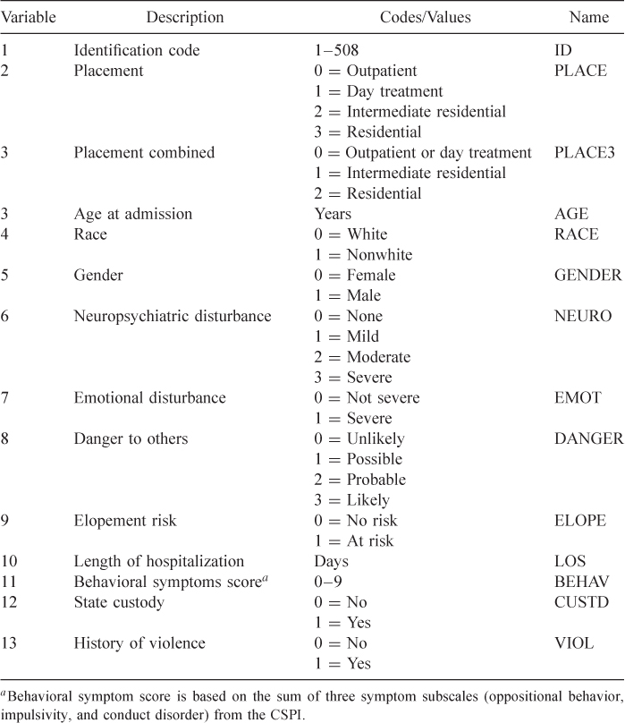
Fontanella et al. (2008) present results from a study of determinants of aftercare placement for psychiatrically hospitalized adolescents and have made the data, suitably modified to protect confidentiality, available to us. It is not our intent to repeat the detailed analyses reported in their paper, but rather to use the data to motivate and describe methods for modeling a multinomial or ordinal scaled outcome using logistic regression models. As such, we selected a subset of variables, which are described in Table 1.8. This data set is referred to as the APS data.
Table 1.8 Code Sheet for Variables in the Adolescent Placement Study
1.6.5 The Burn Injury Study
The April 2008 release (Version 4.0) of the National Burn Repository research dataset (National Burn Repository 2007 Report, Dataset Version 4.0 accessed on 12/05/2008 at: http://www.ameriburn.org/2007NBRAnnualReport.pdf) includes information on a total of 306,304 burn related hospitalizations that occurred between 1973 and 2007. Available information included patient demographics, total burn surface area, presence of inhalation injury, and blinded trauma center identifiers. The outcome of interest is survival to hospital discharge. Osler et al. (2010) selected a subset of approximately 40,000 subjects treated between 2000 and 2007 at 40 different burn facilities to develop a new predictive logistic regression model (see the paper for the details on how this subset was selected). To obtain a much smaller data set for use in this text we over sampled subjects who died in hospital and under sampled subjects who lived to obtain a data set with ![]() and achieve a sample with 15 percent in hospital mortality. As such, all analyses and inferences contained in this text do not apply to the sample of 40,000, the original data from the registry or the population of burn injury patients as a whole. These data are used here to illustrate methods when prediction is the final goal as well as to demonstrate various model building techniques. The variables are described in Table 1.9 and the data are referred to as the BURN1000 data.
and achieve a sample with 15 percent in hospital mortality. As such, all analyses and inferences contained in this text do not apply to the sample of 40,000, the original data from the registry or the population of burn injury patients as a whole. These data are used here to illustrate methods when prediction is the final goal as well as to demonstrate various model building techniques. The variables are described in Table 1.9 and the data are referred to as the BURN1000 data.
Table 1.9 Code Sheet for Variables in the Burn Study

1.6.6 The Myopia Study
Myopia, more commonly referred to as nearsightedness, is an eye condition where an individual has difficulty seeing things at a distance. This condition is primarily because the eyeball is too long. In an eye that sees normally, the image of what is being viewed is transmitted to the back portion of the eye, or retina, and hits the retina to form a clear picture. In the myopic eye, the image focuses in front of the retina, so the resultant image on the retina itself is blurry. The blurry image creates problems with a variety of distance viewing tasks (e.g., reading the blackboard, doing homework, driving, playing sports) and requires wearing glasses or contact lenses to correct the problem. Myopia onset is typically between the ages of 8 and 12 years with cessation of the underlying eye growth that causes it by age 15–16 years.
The risk factors for the development of myopia have been debated for a long time and include genetic factors (e.g., family history of myopia) and the amount and type of visual activity that a child performs (e.g., studying, reading, TV watching, computer or video game playing, and sports/outdoor activity). There is strong evidence that having myopic parents increases the chance that a child will become myopic, and weaker evidence that certain types of visual activities (called near work, e.g., reading) increase the chance that a child will become myopic.
These data are a subset of data from the Orinda Longitudinal Study of Myopia (OLSM), a cohort study of ocular component development and risk factors for the onset of myopia in children, which evolved into the Collaborative Longitudinal Evaluation of Ethnicity and Refractive Error (CLEERE) Study, and both OLSM and CLEERE were funded by the National Institutes of Health/National Eye Institute. OLSM was based at the University of California, Berkeley [see Zadnik et al. (1993, 1994)]. Data collection began in the 1989–1990 school year and continued annually through the 2000–2001 school year. All data about the parts that make up the eye (the ocular components) were collected during an examination during the school day. Data on family history and visual activities were collected yearly in a survey completed by a parent or guardian.
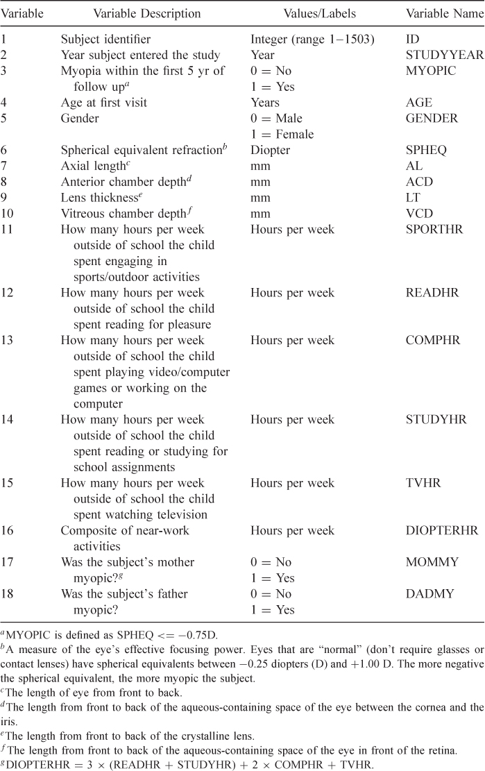
The dataset used in this text is from 618 of the subjects who had at least five years of followup and were not myopic when they entered the study. All data are from their initial exam and includes 17 variables. In addition to the ocular data there is information on age at entry, year of entry, family history of myopia and hours of various visual activities. The ocular data come from a subject's right eye. A subject was coded as myopic if they became myopic at any time during the first five years of followup. We refer to this data set, in Table 1.10, as the MYOPIA data.
Table 1.10 Code Sheet for Variables in the Myopia Study
1.6.7 The NHANES Study
The National Health and Nutrition Examination Survey (NHANES), a major effort of the National Center for Health Statistics, was conceived in the early 1960s to provide nationally representative and reliable data on the health and nutritional status of adults and children in the United States. NHANES has since evolved into a ongoing survey program that provides the best available national estimates of the prevalence of, and risk factors for, targeted diseases in the United States population. The survey collects interview and physical exam data on a nationally representative, multistage probability sample of about 5,000 persons each year, who are chosen to be representative of the civilian, non-institutionalized, population in the US.
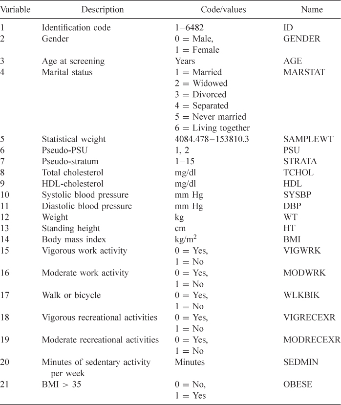
For purposes of illustrating fitting logistic regression models to sample survey data in Section 6.4 we chose selected variables, shown in Table 1.11, from the 2009–2010 cycle of the National Health and Nutrition Examination Study [NHANES III Reference Manuals and Reports (2012)] and made some modifications to the data. We refer to this data set as the NHANES data.
Table 1.11 Variables in the Modified NHANES Data Set
1.6.8 The Polypharmacy Study
In Chapter 9, we illustrate model building with correlated data using data on polypharmacy described in Table 1.12. The outcome of interest is whether the patient is taking drugs from three or more different classes (POLYPHARMACY), and researchers were interested in identifying factors associated with this outcome. We selected a sample of 500 subjects from among only those subjects with observations in each of the seven years data were collected. Based on the suggestions of the principal investigator, we initially treated the covariates for number of inpatient and outpatient mental health visits (MHVs) with categories described in Table 1.12. In addition we added a random number of months to the age, which was recorded only in terms of the year in the original data set. As our data set is a sample, the results in this section do not apply to the original study. We refer to this data set as the POLYPHARM data.
Table 1.12 Code Sheet for the Variables in the Polypharmacy Data Set

Exercises
1. In the ICU data described in Section 1.6.1 the primary outcome variable is vital status at hospital discharge, STA. Clinicians associated with the study felt that a key determinant of survival was the patient's age at admission, AGE.
2. In the Myopia Study described in Section 1.6.2, one variable that is clearly important is the initial value of spherical equivalent refraction.(SPHREQ). Repeat steps (a)–(g) of Exercise 1, but for 2(c) use eight intervals containing approximately equal numbers of subjects (i.e., cut points at 12.5%, 25%, ![]() , etc.).
, etc.).
3. Using the data from the ICU study create a dichotomous variable NONWHITE (![]() if
if ![]() or 3 and
or 3 and ![]() if
if ![]() ). Fit the logistic regression of STA on NONWHITE and show that the 95 percent profile likelihood confidence interval for the coefficient for nonwhite has asymmetry of
). Fit the logistic regression of STA on NONWHITE and show that the 95 percent profile likelihood confidence interval for the coefficient for nonwhite has asymmetry of ![]() and that this interval is 26% wider than the Wald-based interval. This example points out that even when the sample size and number of events are large
and that this interval is 26% wider than the Wald-based interval. This example points out that even when the sample size and number of events are large ![]() , and
, and ![]() there can be substantial asymmetry and differences between the two interval estimators. Explain why this is the case in this example.
there can be substantial asymmetry and differences between the two interval estimators. Explain why this is the case in this example.
1 The remainder of this section is more advanced material that can be skipped on first reading of the text.
2 The term coverage of an interval estimator refers to the percent of time confidence intervals computed in a similar manner contain the true parameter value. Research has shown that when the normality assumption does not hold, Wald-based confidence intervals can be too narrow and thus contain the true parameter with a smaller percentage than the stated confidence coefficient.