
7
Using Regression and Forecasting
One of the most important tasks that a statistician or data scientist has is to generate a systematic understanding of the relationship between two sets of data. This can mean a continuous relationship between two sets of data, where one value depends directly on the value of another variable. Alternatively, it can mean a categorical relationship, where one value is categorized according to another. The tool for working with these kinds of problems is regression. In its most basic form, regression involves fitting a straight line through a scatter plot of the two sets of data and performing some analysis to see how well this line fits the data. Of course, we often need something more sophisticated to model more complex relationships that exist in the real world.
Forecasting typically refers to learning trends in time series data with the aim of predicting values in the future. Time series data is data that evolves over a period of time, and usually exhibits a high degree of noise and oscillatory behavior. Unlike more simple data, time series data usually has complex dependencies between consecutive values; for instance, a value may depend on both of the previous values, and perhaps even on the previous noise. Time series modeling is important across science and economics, and there are a variety of tools for modeling time series data. The basic technique for working with time series data is called autoregressive integrated moving average (ARIMA). This model incorporates two underlying components: an autoregressive (AR) component and a moving average (MA) component, to construct a model for the observed data.
In this chapter, we will learn how to model the relationship between two sets of data, quantify how strong this relationship is, and generate forecasts about other values (the future). Then, we will learn how to use logistic regression, which is a variation of a simple linear model, in classification problems. Finally, we will build models for time series data using ARIMA and build on these models for different kinds of data. We will finish this chapter by using a library called Prophet to automatically generate a model for time series data.
In the first three recipes, we will learn how to perform various kinds of regression to simple data. In the next four recipes, we will learn about various techniques for working with time series data. The final recipe deals with an alternative means of summarizing time series data for various purposes using signature methods.
In this chapter, we will cover the following recipes:
- Using basic linear regression
- Using multilinear regression
- Classifying using logarithmic regression
- Modeling time series data with ARMA
- Forecasting from time series data using ARIMA
- Forecasting seasonal data using ARIMA
- Using Prophet to model time series data
- Using signatures to summarize time series data
Let’s get started!
Technical requirements
In this chapter, as usual, we will need the NumPy package imported under the np alias, the Matplotlib pyplot module imported as plt, and the Pandas package imported as pd. We can do this using the following commands:
import numpy as np
import matplotlib.pyplot as plt
import pandas as pd
We will also need some new packages in this chapter. The statsmodels package is used for regression and time series analysis, the scikit-learn package (sklearn) provides general data science and machine learning tools, and the Prophet package (prophet) is used for automatically modeling time series data. These packages can be installed using your favorite package manager, such as pip:
python3.10 -m pip install statsmodels sklearn prophet
The Prophet package can prove difficult to install on some operating systems because of its dependencies. If installing prophet causes a problem, you might want to try using the Anaconda distribution of Python and its package manager, conda, which handles the dependencies more rigorously:
conda install prophet
Note
Previous versions of the Prophet library (prior to version 1.0) were called fbprophet, whereas the newer versions of Prophet are just prophet.
Finally, we also need a small module called tsdata that is contained in the repository for this chapter. This module contains a series of utilities for producing sample time series data.
The code for this chapter can be found in the Chapter 07 folder of the GitHub repository at https://github.com/PacktPublishing/Applying-Math-with-Python-2nd-Edition/tree/main/Chapter%2007.
Using basic linear regression
Linear regression is a tool for modeling the dependence between two sets of data so that we can eventually use this model to make predictions. The name comes from the fact that we form a linear model (straight line) of one set of data based on a second. In the literature, the variable that we wish to model is frequently called the response variable, and the variable that we are using in this model is the predictor variable.
In this recipe, we’ll learn how to use the statsmodels package to perform simple linear regression to model the relationship between two sets of data.
Getting ready
For this recipe, we will need the statsmodels.api module imported under the sm alias, the NumPy package imported as np, the Matplotlib pyplot module imported as plt, and an instance of a NumPy default random number generator. All this can be achieved with the following commands:
import statsmodels.api as sm
import numpy as np
import matplotlib.pyplot as plt
from numpy.random import default_rng
rng = default_rng(12345)
Let’s see how to use the statsmodels package to perform basic linear regression.
How to do it...
The following steps outline how to use the statsmodels package to perform a simple linear regression on two sets of data:
- First, we generate some example data that we can analyze. We’ll generate two sets of data that will illustrate a good fit and a less good fit:
x = np.linspace(0, 5, 25)
rng.shuffle(x)
trend = 2.0
shift = 5.0
y1 = trend*x + shift + rng.normal(0, 0.5, size=25)
y2 = trend*x + shift + rng.normal(0, 5, size=25)
- A good first step in performing regression analysis is to create a scatter plot of the datasets. We’ll do this on the same set of axes:
fig, ax = plt.subplots()
ax.scatter(x, y1, c="k", marker="x",
label="Good correlation")
ax.scatter(x, y2, c="k", marker="o",
label="Bad correlation")
ax.legend()
ax.set_xlabel("X"),ax.set_ylabel("Y")ax.set_title("Scatter plot of data with best fit lines") - We need to use the sm.add_constant utility routine so that the modeling step will include a constant value:
pred_x = sm.add_constant(x)
- Now, we can create an OLS model for our first set of data and use the fit method to fit the model. We then print a summary of the data using the summary method:
model1 = sm.OLS(y1, pred_x).fit()
print(model1.summary())
- We repeat the model fitting for the second set of data and print the summary:
model2 = sm.OLS(y2, pred_x).fit()
print(model2.summary())
- Now, we create a new range of
 values using linspace that we can use to plot the trend lines on our scatter plot. We need to add the constant column to interact with the models that we have created:
model_x = sm.add_constant(np.linspace(0, 5))
- Next, we use the predict method on the model objects so that we can use the model to predict the response value at each of the
 values we generated in the previous step:
model_y1 = model1.predict(model_x)
model_y2 = model2.predict(model_x)
- Finally, we plot the model data computed in the previous two steps on top of the scatter plot:
ax.plot(model_x[:, 1], model_y1, 'k')
ax.plot(model_x[:, 1], model_y2, 'k--')
The scatter plot, along with the best fit lines (the models) we added, can be seen in the following figure:

Figure 7.1 - Scatter plot of data with lines of best fit computed using least squares regression.
The solid line indicates the line fitted to the well-correlated data (marked by x symbols) and the dashed line indicates the line fitted to the poorly correlated data (marked by dots). We can see in the plot that the two best-fit lines are fairly similar, but the line fitted (dashed) to the data with lots of noise has drifted away from the true model ![]() defined in step 1.
defined in step 1.
How it works...
Elementary mathematics tells us that the equation of a straight line is given by the following:
![]()
Here, ![]() is the value at which the line meets the
is the value at which the line meets the ![]() -axis, usually called the
-axis, usually called the ![]() -intercept, and
-intercept, and ![]() is the gradient of the line. In the linear regression context, we are trying to find a relationship between the response variable,
is the gradient of the line. In the linear regression context, we are trying to find a relationship between the response variable, ![]() , and the predictor variable,
, and the predictor variable, ![]() , which has the form of a straight line so that the following occurs:
, which has the form of a straight line so that the following occurs:
![]()
Here, ![]() and
and ![]() are now parameters that are to be found. We can write this in a different way, as follows:
are now parameters that are to be found. We can write this in a different way, as follows:
![]()
Here, ![]() is an error term, which, in general, depends on
is an error term, which, in general, depends on ![]() . To find the “best” model, we need to find values for the
. To find the “best” model, we need to find values for the ![]() and
and ![]() parameters for which the error term,
parameters for which the error term, ![]() , is minimized (in an appropriate sense). The basic method for finding the values of the parameters such that this error is minimized is the method of least squares, which gives its name to the type of regression used here: ordinary least squares. Once we have used this method to establish some relationship between a response variable and a predictor variable, our next task is to assess how well this model actually represents this relationship. For this, we form the residuals given by the following equation:
, is minimized (in an appropriate sense). The basic method for finding the values of the parameters such that this error is minimized is the method of least squares, which gives its name to the type of regression used here: ordinary least squares. Once we have used this method to establish some relationship between a response variable and a predictor variable, our next task is to assess how well this model actually represents this relationship. For this, we form the residuals given by the following equation:
![]()
We do this for each of the data points, ![]() and
and ![]() . In order to provide a rigorous statistical analysis of how well we have modeled the relationship between the data, we need the residuals to satisfy certain assumptions. First, we need them to be independent in the sense of probability. Second, we need them to be normally distributed about 0 with a common variance (in practice, we can relax these slightly and still make reasonable comments about the accuracy of the model).
. In order to provide a rigorous statistical analysis of how well we have modeled the relationship between the data, we need the residuals to satisfy certain assumptions. First, we need them to be independent in the sense of probability. Second, we need them to be normally distributed about 0 with a common variance (in practice, we can relax these slightly and still make reasonable comments about the accuracy of the model).
In this recipe, we generated response data from the predictor data using a linear relationship. The difference between the two response datasets we created is the “size” of the error at each value. For the first dataset, y1, the residuals were normally distributed with a standard deviation of 0.5, whereas for the second dataset, y2, the residuals have a standard deviation of 5.0. We can see this variability in the scatter plot shown in Figure 7.1, where the data for y1 is generally very close to the best fit line – which closely matches the actual relationship that was used to generate the data – whereas the y2 data is much further from the best-fit line.
The OLS object from the statsmodels package is the main interface for ordinary least squares regression. We provide the response data and the predictor data as arrays. In order to have a constant term in the model, we need to add a column of ones in the predictor data. The sm.add_constant routine is a simple utility for adding this constant column. The fit method of the OLS class computes the parameters for the model and returns a results object (model1 and model2) that contains the parameters for the best fit model. The summary method creates a string containing information about the model and various statistics about the goodness of fit. The predict method applies the model to new data. As the name suggests, it can be used to make predictions using the model.
There are two basic statistics reported in the summary that give us information about the fit. The first is the ![]() value, or the adjusted version, which measures the variability explained by the model against the total variability. This number is defined as follows. First, define the following quantities:
value, or the adjusted version, which measures the variability explained by the model against the total variability. This number is defined as follows. First, define the following quantities:
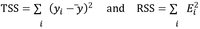
Here, ![]() are the residuals defined previously and
are the residuals defined previously and ![]() is the mean of the data. We then define
is the mean of the data. We then define ![]() and its adjusted counterpart:
and its adjusted counterpart:

In the latter equation, ![]() is the size of the sample and
is the size of the sample and ![]() is the number of variables in the model (including the
is the number of variables in the model (including the ![]() -intercept
-intercept ![]() ). A higher value indicates a better fit, with a best possible value of 1. Note that the ordinary
). A higher value indicates a better fit, with a best possible value of 1. Note that the ordinary ![]() value tends to be overly optimistic, especially when the model contains more variables, so it is usually better to look at the adjusted version.
value tends to be overly optimistic, especially when the model contains more variables, so it is usually better to look at the adjusted version.
The second is the F statistic p-value. This is a hypothesis test that at least one of the coefficients of the model is non-zero. As with ANOVA testing (see Testing Hypotheses with ANOVA, Chapter 6), a small p-value indicates that the model is significant, meaning that the model is more likely to accurately model the data.
In this recipe, the first model, model1, has an adjusted ![]() value of 0.986, indicating that the model very closely fits the data, and a p-value of 6.43e-19, indicating high significance. The second model has an adjusted
value of 0.986, indicating that the model very closely fits the data, and a p-value of 6.43e-19, indicating high significance. The second model has an adjusted ![]() value of 0.361, which indicates that the model less closely fits the data, and a p-value of 0.000893, which also indicates high significance. Even though the second model less closely fits the data, in terms of statistics, that is not to say that it is not useful. The model is still significant, although less so than the first model, but it doesn’t account for all of the variability (or at least a significant portion of it) in the data. This could be indicative of additional (non-linear) structures in the data, or that the data is less correlated, which means there is a weaker relationship between the response and predictor data (due to the way we constructed the data, we know that the latter is true).
value of 0.361, which indicates that the model less closely fits the data, and a p-value of 0.000893, which also indicates high significance. Even though the second model less closely fits the data, in terms of statistics, that is not to say that it is not useful. The model is still significant, although less so than the first model, but it doesn’t account for all of the variability (or at least a significant portion of it) in the data. This could be indicative of additional (non-linear) structures in the data, or that the data is less correlated, which means there is a weaker relationship between the response and predictor data (due to the way we constructed the data, we know that the latter is true).
There’s more...
Simple linear regression is a good general-purpose tool in a statistician’s toolkit. It is excellent for finding the nature of the relationship between two sets of data that are known (or suspected) to be connected in some way. The statistical measurement of how much one set of data depends on another is called correlation. We can measure correlation using a correlation coefficient, such as Spearman’s rank correlation coefficient. A high positive correlation coefficient indicates a strong positive relationship between the data, such as that seen in this recipe, while a high negative correlation coefficient indicates a strong negative relationship, where the slope of the best-fit line through the data is negative. A correlation coefficient of 0 means that the data is not correlated: there is no relationship between the data.
If the sets of data are clearly related but not in a linear (straight line) relationship, then it might follow a polynomial relationship where, for example, one value is related to the other squared. Sometimes, you can apply a transformation, such as a logarithm, to one set of data and then use linear regression to fit the transformed data. Logarithms are especially useful when there is a power-law relationship between the two sets of data.
The scikit-learn package also provides facilities for performing ordinary least squares regression. However, their implementation does not offer an easy way to generate goodness-of-fit statistics, which are often useful when performing a linear regression in isolation. The summary method on the OLS object is very convenient for producing all the required fitting information, along with the estimated coefficients.
Using multilinear regression
Simple linear regression, as seen in the previous recipe, is excellent for producing simple models of a relationship between one response variable and one predictor variable. Unfortunately, it is far more common to have a single response variable that depends on many predictor variables. Moreover, we might not know which variables from a collection make good predictor variables. For this task, we need multilinear regression.
In this recipe, we will learn how to use multilinear regression to explore the relationship between a response variable and several predictor variables.
Getting ready
For this recipe, we will need the NumPy package imported as np, the Matplotlib pyplot module imported as plt, the Pandas package imported as pd, and an instance of the NumPy default random number generator created using the following commands:
from numpy.random import default_rng
rng = default_rng(12345)
We will also need the statsmodels.api module imported as sm, which can be imported using the following command:
import statsmodels.api as sm
Let’s see how to fit a multilinear regression model to some data.
How to do it...
The following steps show you how to use multilinear regression to explore the relationship between several predictors and a response variable:
- First, we need to create the predictor data to analyze. This will take the form of a Pandas DataFrame with four terms. We will add the constant term at this stage by adding a column of ones:
p_vars = pd.DataFrame({"const": np.ones((100,)),
"X1": rng.uniform(0, 15, size=100),
"X2": rng.uniform(0, 25, size=100),
"X3": rng.uniform(5, 25, size=100)
})
- Next, we will generate the response data using only the first two variables:
residuals = rng.normal(0.0, 12.0, size=100)
Y = -10.0 + 5.0*p_vars["X1"] - 2.0*p_vars["X2"] + residuals
- Now, we’ll produce scatter plots of the response data against each of the predictor variables:
fig, (ax1, ax2, ax3) = plt.subplots(1, 3, sharey=True,
tight_layout=True)
ax1.scatter(p_vars["X1"], Y, c="k")
ax2.scatter(p_vars["X2"], Y, c="k")
ax3.scatter(p_vars["X3"], Y, c="k")
- Then, we’ll add axis labels and titles to each scatter plot since this is good practice:
ax1.set_title("Y against X1")ax1.set_xlabel("X1")ax1.set_ylabel("Y")ax2.set_title("Y against X2")ax2.set_xlabel("X2")ax3.set_title("Y against X3")ax3.set_xlabel("X3")
The resulting plots can be seen in the following figure:
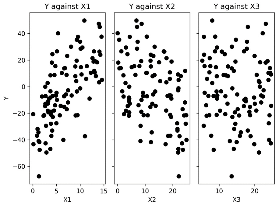
Figure 7.2 - Scatter plots of the response data against each of the predictor variables
As we can see, there appears to be some correlation between the response data and the first two predictor columns, X1 and X2. This is what we expect, given how we generated the data.
- We use the same OLS class to perform multilinear regression; that is, providing the response array and the predictor DataFrame:
model = sm.OLS(Y, p_vars).fit()
print(model.summary())
The first half of the output of the print statement is as follows:
                   OLS Regression Results
===========================================
Dep. Variable:        y            R-squared:0.769
Model:              OLS             Adj. R-squared:0.764
Method: Least Squares  F-statistic:161.5
Date: Fri, 25 Nov 2022 Prob (F-statistic):1.35e-31
Time: 12:38:40      Log-Likelihood:-389.48
No. Observations: 100 AIC:        785.0
Df Residuals: 97              BIC:     792.8
Df Model: 2
Covariance Type:  nonrobust
This gives us a summary of the model, various parameters, and various goodness-of-fit characteristics such as the R-squared values (0.77 and 0.762), which indicate that the fit is reasonable but not very good. The second half of the output contains information about the estimated coefficients:
=========================================
         coef           std err      t     P>|t|  [0.025    0.975]
-----------------------------------------------------------------------
const -11.1058  2.878  -3.859 0.000  -16.818  -5.393
X1      4.7245  0.301  15.672   0.00    4.126      5.323
X2     -1.9050  0.164 -11.644  0.000   -2.230   -1.580
=========================================
Omnibus:           0.259        Durbin-Watson:     1.875
Prob(Omnibus): 0.878       Jarque-Bera (JB):  0.260
Skew: 0.115             Prob(JB):         0.878
Kurtosis: 2.904         Cond. No          38.4
=========================================
Notes:
[1] Standard Errors assume that the covariance matrix of the errors is correctly specified.
In the summary data, we can see that the X3 variable is not significant since it has a p-value of 0.66.
- Since the third predictor variable is not significant, we eliminate this column and perform the regression again:
second_model = sm.OLS(
Y, p_vars.loc[:, "const":"X2"]).fit()
print(second_model.summary())
This results in a small increase in the goodness-of-fit statistics.
How it works...
Multilinear regression works in much the same way as simple linear regression. We follow the same procedure here as in the previous recipe, where we use the statsmodels package to fit a multilinear model to our data. Of course, there are some differences behind the scenes. The model we produce using multilinear regression is very similar in form to the simple linear model from the previous recipe. It has the following form:
![]()
Here, ![]() is the response variable,
is the response variable, ![]() represents the predictor variables,
represents the predictor variables, ![]() is the error term, and
is the error term, and ![]() is the parameters to be computed. The same requirements are also necessary for this context: residuals must be independent and normally distributed with a mean of 0 and a common standard deviation.
is the parameters to be computed. The same requirements are also necessary for this context: residuals must be independent and normally distributed with a mean of 0 and a common standard deviation.
In this recipe, we provided our predictor data as a Pandas DataFrame rather than a plain NumPy array. Notice that the names of the columns have been adopted in the summary data that we printed. Unlike the first recipe, Using basic linear regression, we included the constant column in this DataFrame, rather than using the add_constant utility from statsmodels.
In the output of the first regression, we can see that the model is a reasonably good fit with an adjusted ![]() value of 0.762, and is highly significant (we can see this by looking at the regression F statistic p-value). However, looking closer at the individual parameters, we can see that both of the first two predictor values are significant, but the constant and the third predictor are less so. In particular, the third predictor parameter, X3, is not significantly different from 0 and has a p-value of 0.66. Given that our response data was constructed without using this variable, this shouldn’t come as a surprise. In the final step of the analysis, we repeat the regression without the predictor variable, X3, which is a mild improvement to the fit.
value of 0.762, and is highly significant (we can see this by looking at the regression F statistic p-value). However, looking closer at the individual parameters, we can see that both of the first two predictor values are significant, but the constant and the third predictor are less so. In particular, the third predictor parameter, X3, is not significantly different from 0 and has a p-value of 0.66. Given that our response data was constructed without using this variable, this shouldn’t come as a surprise. In the final step of the analysis, we repeat the regression without the predictor variable, X3, which is a mild improvement to the fit.
Classifying using logarithmic regression
Logarithmic regression solves a different problem from ordinary linear regression. It is commonly used for classification problems where, typically, we wish to classify data into two distinct groups, according to a number of predictor variables. Underlying this technique is a transformation that’s performed using logarithms. The original classification problem is transformed into a problem of constructing a model for the log-odds. This model can be completed with simple linear regression. We apply the inverse transformation to the linear model, which leaves us with a model of the probability that the desired outcome will occur, given the predictor data. The transform we apply here is called the logistic function, which gives its name to the method. The probability we obtain can then be used in the classification problem we originally aimed to solve.
In this recipe, we will learn how to perform logistic regression and use this technique in classification problems.
Getting ready
For this recipe, we will need the NumPy package imported as np, the Matplotlib pyplot module imported as plt, the Pandas package imported as pd, and an instance of the NumPy default random number generator to be created using the following commands:
from numpy.random import default_rng
rng = default_rng(12345)
We also need several components from the scikit-learn package to perform logistic regression. These can be imported as follows:
from sklearn.linear_model import LogisticRegression
from sklearn.metrics import classification_report
How to do it...
Follow these steps to use logistic regression to solve a simple classification problem:
- First, we need to create some sample data that we can use to demonstrate how to use logistic regression. We start by creating the predictor variables:
df = pd.DataFrame({"var1": np.concatenate([
rng.normal(3.0, 1.5, size=50),
rng.normal(-4.0, 2.0, size=50)]),
"var2": rng.uniform(size=100),
"var3": np.concatenate([
rng.normal(-2.0, 2.0, size=50),
rng.normal(1.5, 0.8, size=50)])
})
- Now, we use two of our three predictor variables to create our response variable as a series of Boolean values:
score = 4.0 + df["var1"] - df["var3"]
Y = score >= 0
- Next, we scatterplot the points, styled according to the response variable, of the var3 data against the var1 data, which are the variables used to construct the response variable:
fig1, ax1 = plt.subplots()
ax1.plot(df.loc[Y, "var1"], df.loc[Y, "var3"],
"ko", label="True data")
ax1.plot(df.loc[~Y, "var1"], df.loc[~Y, "var3"],
"kx", label="False data")
ax1.legend()
ax1.set_xlabel("var1")ax1.set_ylabel("var3")ax1.set_title("Scatter plot of var3 against var1")
The resulting plot can be seen in the following figure:

Figure 7.3 – Scatter plot of the var3 data against var1, with classification marked
- Next, we create a LogisticRegression object from the scikit-learn package and fit the model to our data:
model = LogisticRegression()
model.fit(df, Y)
- Next, we prepare some extra data, different from what we used to fit the model, to test the accuracy of our model:
test_df = pd.DataFrame({"var1": np.concatenate([
rng.normal(3.0, 1.5, size=50),
rng.normal(-4.0, 2.0, size=50)]),
"var2": rng.uniform(size=100),
"var3": np.concatenate([
rng.normal(-2.0, 2.0, size=50),
rng.normal(1.5, 0.8, size=50)])
})
test_scores = 4.0 + test_df["var1"] - test_df["var3"]
test_Y = test_scores >= 0
- Then, we generate predicted results based on our logistic regression model:
test_predicts = model.predict(test_df)
- Finally, we use the classification_report utility from scikit-learn to print a summary of predicted classification against known response values to test the accuracy of the model. We print this summary to the Terminal:
print(classification_report(test_Y, test_predicts))
The report that’s generated by this routine looks as follows:
              precision    recall      f1-score   support
       False       0.82      1.00        0.90        18
        True        1.00      0.88        0.93        32
accuracy                     0.92                   50
   macro avg     0.91      0.94       0.92         50
weighted avg    0.93      0.92       0.92         50
The report here contains information about the performance of the classification model on the test data. We can see that the reported precision and recall are good, indicating that there were relatively few false positive and false negative identifications.
How it works...
Logistic regression works by forming a linear model of the log-odds ratio (or logit), which, for a single predictor variable, ![]() , has the following form:
, has the following form:

Here, ![]() represents the probability of a true outcome in response to the given predictor,
represents the probability of a true outcome in response to the given predictor, ![]() . Rearranging this gives a variation of the logistic function for the probability:
. Rearranging this gives a variation of the logistic function for the probability:

The parameters for the log-odds are estimated using a maximum likelihood method.
The LogisticRegression class from the linear_model module in scikit-learn is an implementation of logistic regression that is very easy to use. First, we create a new model instance of this class, with any custom parameters that we need, and then use the fit method on this object to fit (or train) the model to the sample data. Once this fitting is done, we can access the parameters that have been estimated using the get_params method.
The predict method on the fitted model allows us to pass in new (unseen) data and make predictions about the classification of each sample. We could also get the probability estimates that are actually given by the logistic function using the predict_proba method.
Once we have built a model for predicting the classification of data, we need to validate the model. This means we have to test the model with some previously unseen data and check whether it correctly classifies the new data. For this, we can use classification_report, which takes a new set of data and the predictions generated by the model and computes several summary values about the performance of the model. The first reported value is the precision, which is the ratio of the number of true positives to the number of predicted positives. This measures how well the model avoids labeling values as positive when they are not. The second reported value is the recall, which is the ratio of the number of true positives to the number of true positives plus the number of false negatives. This measures the ability of the model to find positive samples within the collection. A related score (not included in the report) is the accuracy, which is the ratio of the number of correct classifications to the total number of classifications. This measures the ability of the model to correctly label samples.
The classification report we generated using the scikit-learn utility performs a comparison between the predicted results and the known response values. This is a common method for validating a model before using it to make actual predictions. In this recipe, we saw that the reported precision for each of the categories (True and False) was 1.00, indicating that the model performed perfectly in predicting the classification with this data. In practice, it is unlikely that the precision of a model will be 100%.
There’s more...
There are lots of packages that offer tools for using logistic regression for classification problems. The statsmodels package has the Logit class for creating logistic regression models. We used the scikit-learn package in this recipe, which has a similar interface. scikit-learn is a general-purpose machine learning library and has a variety of other tools for classification problems.
Modeling time series data with ARMA
Time series, as the name suggests, track a value over a sequence of distinct time intervals. They are particularly important in the finance industry, where stock values are tracked over time and used to make predictions – known as forecasting – of the value at some point in the future. Good predictions coming from this kind of data can be used to make better investments. Time series also appear in many other common situations, such as weather monitoring, medicine, and any places where data is derived from sensors over time.
Time series, unlike other types of data, do not usually have independent data points. This means that the methods that we use for modeling independent data will not be particularly effective. Thus, we need to use alternative techniques to model data with this property. There are two ways in which a value in a time series can depend on previous values. The first is where there is a direct relationship between the value and one or more previous values. This is the autocorrelation property and is modeled by an AR model. The second is where the noise that’s added to the value depends on one or more previous noise terms. This is modeled by an MA model. The number of terms involved in either of these models is called the order of the model.
In this recipe, we will learn how to create a model for stationary time series data with ARMA terms.
Getting ready
For this recipe, we need the Matplotlib pyplot module imported as plt and the statsmodels package api module imported as sm. We also need to import the generate_sample_data routine from the tsdata package from this book’s repository, which uses NumPy and Pandas to generate sample data for analysis:
from tsdata import generate_sample_data
To avoid repeatedly setting colors in plotting functions, we do some one-time setup to set the plotting color here:
from matplotlib.rcsetup import cycler
plt.rc("axes", prop_cycle=cycler(c="k"))
With this set up, we can now see how to generate an ARMA model for some time series data.
How to do it...
Follow these steps to create an ARMA model for stationary time series data:
- First, we need to generate the sample data that we will analyze:
sample_ts, _ = generate_sample_data()
- As always, the first step in the analysis is to produce a plot of the data so that we can visually identify any structure:
ts_fig, ts_ax = plt.subplots()
sample_ts.plot(ax=ts_ax, label="Observed",
ls="--", alpha=0.4)
ts_ax.set_title("Time series data")ts_ax.set_xlabel("Date")ts_ax.set_ylabel("Value")
The resulting plot can be seen in the following figure:

Figure 7.4 - Plot of the time series data that we will analyze (there doesn’t appear to be a trend in this data)
Here, we can see that there doesn’t appear to be an underlying trend, which means that the data is likely to be stationary (a time series is said to be stationary if its statistical properties do not vary with time. This often manifests in the form of an upward or downward trend).
- Next, we compute the augmented Dickey-Fuller test. This is a hypothesis test for whether a time series is stationary or not. The null hypothesis is that the time series is not stationary:
adf_results = sm.tsa.adfuller(sample_ts)
adf_pvalue = adf_results[1]
print("Augmented Dickey-Fuller test:
P-value:",
adf_pvalue)
The reported adf_pvalue is 0.000376 in this case, so we reject the null hypothesis and conclude that the series is stationary.
- Next, we need to determine the order of the model that we should fit. For this, we’ll plot the autocorrelation function (ACF) and the partial autocorrelation function (PACF) for the time series:
ap_fig, (acf_ax, pacf_ax) = plt.subplots(
2, 1, tight_layout=True)
sm.graphics.tsa.plot_acf(sample_ts, ax=acf_ax,
title="Observed autocorrelation")
sm.graphics.tsa.plot_pacf(sample_ts, ax=pacf_ax,
title="Observed partial autocorrelation")
acf_ax.set_xlabel("Lags")pacf_ax.set_xlabel("Lags")pacf_ax.set_ylabel("Value")acf_ax.set_ylabel("Value")
The plots of the ACF and PACF for our time series can be seen in the following figure. These plots suggest the existence of both AR and MA processes:
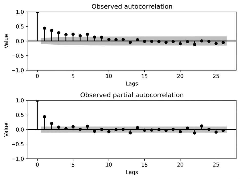
Figure 7.5 - The ACF and PACF for the sample time series data
- Next, we create an ARMA model for the data, using the ARIMA class from the tsa module. This model will have an order 1 AR component and an order 1 MA component:
arma_model = sm.tsa.ARIMA(sample_ts, order=(1, 0, 1))
- Now, we fit the model to the data and get the resulting model. We print a summary of these results to the Terminal:
arma_results = arma_model.fit()
print(arma_results.summary())
- The summary data given for the fitted model is as follows:
ARMA Model Results
=========================================
Dep. Variable: y No. Observations: 366
Model: ARMA(1, 1) Log Likelihood -513.038
Method: css-mle S.D. of innovations
0.982
Date: Fri, 01 May 2020 AIC 1034.077
Time: 12:40:00 BIC 1049.687
Sample: 01-01-2020 HQIC 1040.280
- 12-31-2020
==================================================
coef std err z P>|z| [0.025 0.975]
---------------------------------------------------------------------
const -0.0242 0.143 -0.169 0.866 -0.305 0.256
ar.L1.y 0.8292 0.057 14.562 0.000 0.718 0.941
ma.L1.y -0.5189 0.090 -5.792 0.000 -0.695 -0.343
Roots
=========================================
Real Imaginary Modulus
Frequency
---------------------------------------------------------
AR.1 1.2059 +0.0000j 1.2059
0.0000
MA.1 1.9271 +0.0000j 1.9271
0.0000
---------------------------------------------------
Here, we can see that both of the estimated parameters for the AR and MA components are significantly different from 0. This is because the value in the P >|z| column is 0 to 3 decimal places.
- Next, we need to verify that there is no additional structure remaining in the residuals (error) of the predictions from our model. For this, we plot the ACF and PACF of the residuals:
residuals = arma_results.resid
rap_fig, (racf_ax, rpacf_ax) = plt.subplots(
2, 1, tight_layout=True)
sm.graphics.tsa.plot_acf(residuals, ax=racf_ax,
title="Residual autocorrelation")
sm.graphics.tsa.plot_pacf(residuals, ax=rpacf_ax,
title="Residual partial autocorrelation")
racf_ax.set_xlabel("Lags")rpacf_ax.set_xlabel("Lags")rpacf_ax.set_ylabel("Value")racf_ax.set_ylabel("Value")
The ACF and PACF of the residuals can be seen in the following figure. Here, we can see that there are no significant spikes at lags other than 0, so we conclude that there is no structure remaining in the residuals:

Figure 7.6 - The ACF and PACF for the residuals from our model
- Now that we have verified that our model is not missing any structure, we plot the values that are fitted to each data point on top of the actual time series data to see whether the model is a good fit for the data. We plot this model in the plot we created in step 2:
fitted = arma_results.fittedvalues
fitted.plot(ax=ts_ax, label="Fitted")
ts_ax.legend()
The updated plot can be seen in the following figure:

Figure 7.7 – Plot of the fitted time series data over the observed time series data
The fitted values give a reasonable approximation of the behavior of the time series but reduce the noise from the underlying structure.
How it works...
The ARMA model that we used in this recipe is a basic means of modeling the behavior of stationary time series. The two parts of an ARMA model are the AR and MA parts, which model the dependence of the terms and noise, respectively, on previous terms and noise. In practice, time series are usually not stationary, and we have to perform some kind of transformation to make this the case before we can fit an ARMA model.
An order 1 AR model has the following form:
![]()
Here, ![]() represents the parameters and
represents the parameters and ![]() is the noise at a given step. The noise is usually assumed to be normally distributed with a mean of 0 and a standard deviation that is constant across all the time steps. The
is the noise at a given step. The noise is usually assumed to be normally distributed with a mean of 0 and a standard deviation that is constant across all the time steps. The ![]() value represents the value of the time series at the time step,
value represents the value of the time series at the time step, ![]() . In this model, each value depends on the previous value, although it can also depend on some constants and some noise. The model will give rise to a stationary time series precisely when the
. In this model, each value depends on the previous value, although it can also depend on some constants and some noise. The model will give rise to a stationary time series precisely when the ![]() parameter lies strictly between -1 and 1.
parameter lies strictly between -1 and 1.
An order 1 MA model is very similar to an AR model and is given by the following equation:
![]()
Here, the variants of ![]() are parameters. Putting these two models together gives us an ARMA(1,1) model, which has the following form:
are parameters. Putting these two models together gives us an ARMA(1,1) model, which has the following form:
![]()
In general, we can have an ARMA(p,q) model that has an order ![]() AR component and an order q MA component. We usually refer to the quantities,
AR component and an order q MA component. We usually refer to the quantities, ![]() and
and ![]() , as the orders of the model.
, as the orders of the model.
Determining the orders of the AR and MA components is the most tricky aspect of constructing an ARMA model. The ACF and PACF give some information about this, but even then, it can be quite difficult. For example, an AR process will show some kind of decay or oscillating pattern on the ACF as lag increases, and a small number of peaks on the PACF and values that are not significantly different from zero beyond that. The number of peaks that appear on the PAF plot can be taken as the order of the process. For an MA process, the reverse is true. There is usually a small number of significant peaks on the ACF plot, and a decay or oscillating pattern on the PACF plot. Of course, sometimes, this isn’t obvious.
In this recipe, we plotted the ACF and PACF for our sample time series data. In the autocorrelation plot in Figure 7.5 (top), we can see that the peaks decay rapidly until they lie within the confidence interval of zero (meaning they are not significant). This suggests the presence of an AR component. On the partial autocorrelation plot in Figure 7.5 (bottom), we can see that there are only two peaks that can be considered not zero, which suggests an AR process of order 1 or 2. You should try to keep the order of the model as small as possible. Due to this, we chose an order 1 AR component. With this assumption, the second peak on the partial autocorrelation plot is indicative of decay (rather than an isolated peak), which suggests the presence of an MA process. To keep the model simple, we try an order 1 MA process. This is how the model that we used in this recipe was decided on. Notice that this is not an exact process, and you might have decided differently.
We use the augmented Dickey-Fuller test to test the likelihood that the time series that we have observed is stationary. This is a statistical test, such as those seen in Chapter 6, Working with Data and Statistics, that generates a test statistic from the data. This test statistic, in turn, determines a p-value that is used to determine whether to accept or reject the null hypothesis. For this test, the null hypothesis is that a unit root is present in the time series that’s been sampled. The alternative hypothesis – the one we are really interested in – is that the observed time series is (trend) stationary. If the p-value is sufficiently small, then we can conclude with the specified confidence that the observed time series is stationary. In this recipe, the p-value was 0.000 to 3 decimal places, which indicates a strong likelihood that the series is stationary. Stationarity is an essential assumption for using the ARMA model for the data.
Once we have determined that the series is stationary, and decided on the orders of the model, we have to fit the model to the sample data that we have. The parameters of the model are estimated using a maximum likelihood estimator. In this recipe, the learning of the parameters is done using the fit method, in step 6.
The statsmodels package provides various tools for working with time series, including utilities for calculating – and plotting – ACF and PACF of time series data, various test statistics, and creating ARMA models for time series. There are also some tools for automatically estimating the order of the model.
We can use the Akaike information criterion (AIC), Bayesian information criterion (BIC), and Hannan-Quinn Information Criterion (HQIC) quantities to compare this model to other models to see which model best describes the data. A smaller value is better in each case.
Note
When using ARMA to model time series data, as in all kinds of mathematical modeling tasks, it is best to pick the simplest model that describes the data to the extent that is needed. For ARMA models, this usually means picking the smallest order model that describes the structure of the observed data.
There’s more...
Finding the best combination of orders for an ARMA model can be quite difficult. Often, the best way to fit a model is to test multiple different configurations and pick the order that produces the best fit. For example, we could have tried ARMA(0,1) or ARMA(1, 0) in this recipe, and compared it to the ARMA(1,1) model we used to see which produced the best fit by considering the AIC statistic reported in the summary. In fact, if we build these models, we will see that the AIC value for ARMA(1,1) – the model we used in this recipe – is the “best” of these three models.
Forecasting from time series data using ARIMA
In the previous recipe, we generated a model for a stationary time series using an ARMA model, which consists of an AR component and an MA component. Unfortunately, this model cannot accommodate time series that have some underlying trend; that is, they are not stationary time series. We can often get around this by differencing the observed time series one or more times until we obtain a stationary time series that can be modeled using ARMA. The incorporation of differencing into an ARMA model is called an ARIMA model.
Differencing is the process of computing the difference between consecutive terms in a sequence of data – so, applying first-order differencing amounts to subtracting the value at the current step from the value at the next step (![]() ). This has the effect of removing the underlying upward or downward linear trend from the data. This helps to reduce an arbitrary time series to a stationary time series that can be modeled using ARMA. Higher-order differencing can remove higher-order trends to achieve similar effects.
). This has the effect of removing the underlying upward or downward linear trend from the data. This helps to reduce an arbitrary time series to a stationary time series that can be modeled using ARMA. Higher-order differencing can remove higher-order trends to achieve similar effects.
An ARIMA model has three parameters, usually labeled ![]() ,
, ![]() , and
, and ![]() . The
. The ![]() and
and ![]() order parameters are the order of the AR component and the MA component, respectively, just as they are for the ARMA model. The third order parameter,
order parameters are the order of the AR component and the MA component, respectively, just as they are for the ARMA model. The third order parameter, ![]() , is the order of differencing to be applied. An ARIMA model with these orders is usually written as ARIMA (
, is the order of differencing to be applied. An ARIMA model with these orders is usually written as ARIMA (![]() ,
, ![]() ,
, ![]() ). Of course, we will need to determine what order differencing should be included before we start fitting the model.
). Of course, we will need to determine what order differencing should be included before we start fitting the model.
In this recipe, we will learn how to fit an ARIMA model to a non-stationary time series and use this model to generate forecasts about future values.
Getting ready
For this recipe, we will need the NumPy package imported as np, the Pandas package imported as pd, the Matplotlib pyplot module as plt, and the statsmodels.api module imported as sm. We will also need the utility for creating sample time series data from the tsdata module, which is included in this book’s repository:
from tsdata import generate_sample_data
As in the previous recipe, we use the Matplotlib rcparams to set the color for all plots in the recipe:
from matplotlib.rcsetup import cycler
plt.rc("axes", prop_cycle=cycler(c="k"))
How to do it...
The following steps show you how to construct an ARIMA model for time series data and use this model to make forecasts:
- First, we load the sample data using the generate_sample_data routine:
sample_ts, test_ts = generate_sample_data(
trend=0.2, undiff=True)
- As usual, the next step is to plot the time series so that we can visually identify the trend of the data:
ts_fig, ts_ax = plt.subplots(tight_layout=True)
sample_ts.plot(ax=ts_ax, label="Observed")
ts_ax.set_title("Training time series data")ts_ax.set_xlabel("Date")ts_ax.set_ylabel("Value")
The resulting plot can be seen in the following figure. As we can see, there is a clear upward trend in the data, so the time series is certainly not stationary:

Figure 7.8 – Plot of the sample time series
There is an obvious positive trend in the data.
- Next, we difference the series to see whether one level of differencing is sufficient to remove the trend:
diffs = sample_ts.diff().dropna()
- Now, we plot the ACF and PACF for the differenced time series:
ap_fig, (acf_ax, pacf_ax) = plt.subplots(2, 1,
tight_layout=True)
sm.graphics.tsa.plot_acf(diffs, ax=acf_ax)
sm.graphics.tsa.plot_pacf(diffs, ax=pacf_ax)
acf_ax.set_ylabel("Value")acf_ax.set_xlabel("Lag")pacf_ax.set_xlabel("Lag")pacf_ax.set_ylabel("Value")
The ACF and PACF can be seen in the following figure. We can see that there do not appear to be any trends left in the data and that there appears to be both an AR component and an MA component:

Figure 7.9 - ACF and PACF for the differenced time series
- Now, we construct the ARIMA model with order 1 differencing, an AR component, and an MA component. We fit this to the observed time series and print a summary of the model:
model = sm.tsa.ARIMA(sample_ts, order=(1,1,1))
fitted = model.fit()
print(fitted.summary())
The summary information that’s printed looks as follows:
             SARIMAX Results
===========================================
Dep. Variable:      y   No.  Observations:  366
Model:  ARIMA(1, 0, 1)         Log Likelihood  -513.038
Date:  Fri, 25 Nov 2022         AIC            1034.077
Time:              13:17:24         BIC            1049.687
Sample:      01-01-2020        HQIC           1040.280
                 - 12-31-2020
Covariance Type:                  opg
=========================================
              coef    std err     z       P>|z|   [0.025   0.975]
-----------------------------------------------------------------------
const  -0.0242  0.144  -0.168  0.866   -0.307   0.258
ar.L1   0.8292  0.057  14.512  0.000   0.717    0.941
ma.L1  -0.5189  0.087  -5.954  0.000  -0.690  -0.348
sigma2  0.9653  0.075  12.902  0.000  0.819   1.112
=========================================
Ljung-Box (L1) (Q):      0.04   Jarque-Bera (JB):  0.59
Prob(Q):                        0.84  Prob(JB):                0.74
Heteroskedasticity (H): 1.15   Skew:                    -0.06
Prob(H) (two-sided):     0.44   Kurtosis:                 2.84
=========================================
Warnings:
[1] Covariance matrix calculated using the outer product of gradients (complex-step).
Here, we can see that all 3 of our estimated coefficients are significantly different from 0 since all three have 0 to 3 decimal places in the P>|z| column.
- Now, we can use the get_forecast method to generate predictions of future values and generate a summary DataFrame from these predictions. This also returns the standard error and confidence intervals for predictions:
forecast =fitted.get_forecast(steps=50).summary_frame()
- Next, we plot the forecast values and their confidence intervals on the figure containing the time series data:
forecast["mean"].plot(
ax=ts_ax, label="Forecast", ls="--")
ts_ax.fill_between(forecast.index,
forecast["mean_ci_lower"],
forecast["mean_ci_upper"],
alpha=0.4)
- Finally, we add the actual future values to generate, along with the sample in step 1, to the plot (it might be easier if you repeat the plot commands from step 1 to regenerate the whole plot here):
test_ts.plot(ax=ts_ax, label="Actual", ls="-.")
ts_ax.legend()
The final plot containing the time series with the forecast and the actual future values can be seen in the following figure:

Figure 7.10 - Sample time series with forecast values and actual future values for comparison
Here, we can see that the actual future values are within the confidence interval for the forecast values.
How it works...
The ARIMA model – with orders ![]() ,
, ![]() , and
, and ![]() – is simply an ARMA (
– is simply an ARMA (![]() ,
,![]() ) model that’s applied to a time series. This is obtained by applying differencing of order
) model that’s applied to a time series. This is obtained by applying differencing of order ![]() to the original time series data. It is a fairly simple way to generate a model for time series data. The statsmodels ARIMA class handles the creation of a model, while the fit method fits this model to the data.
to the original time series data. It is a fairly simple way to generate a model for time series data. The statsmodels ARIMA class handles the creation of a model, while the fit method fits this model to the data.
The model is fit to the data using a maximum likelihood method and the final estimates for the parameters – in this case, one parameter for the AR component, one for the MA component, the constant trend parameter, and the variance of the noise. These parameters are reported in the summary. From this output, we can see that the estimates for the AR coefficient (0.9567) and the MA constant (-0.6407) are very good approximations of the true estimates that were used to generate the data, which were 0.8 for the AR coefficient and -0.5 for the MA coefficient. These parameters are set in the generate_sample_data routine from the tsdata.py file in the code repository for this chapter. This generates the sample data in step 1. You might have noticed that the constant parameter (1.0101) is not 0.2, as specified in the generate_sample_data call in step 1. In fact, it is not so far from the actual drift of the time series.
The get_forecast method on the fitted model (the output of the fit method) uses the model to make predictions about the value after a given number of steps. In this recipe, we forecast for up to 50 time steps beyond the range of the sample time series. The output of the command in step 6 is a DataFrame containing the forecast values, the standard error for the forecasts, and the upper and lower bounds for the confidence interval (by default, 95% confidence) of the forecasts.
When you construct an ARIMA model for time series data, you need to make sure you use the smallest order differencing that removes the underlying trend. Applying more differencing than is necessary is called over-differencing and can lead to problems with the model.
Forecasting seasonal data using ARIMA
Time series often display periodic behavior so that peaks or dips in the value appear at regular intervals. This behavior is called seasonality in the analysis of time series. The methods we have used thus far in this chapter to model time series data obviously do not account for seasonality. Fortunately, it is relatively easy to adapt the standard ARIMA model to incorporate seasonality, resulting in what is sometimes called a SARIMA model.
In this recipe, we will learn how to model time series data that includes seasonal behavior and use this model to produce forecasts.
Getting ready
For this recipe, we will need the NumPy package imported as np, the Pandas package imported as pd, the Matplotlib pyplot module as plt, and the statsmodels api module imported as sm. We will also need the utility for creating sample time series data from the tsdata module, which is included in this book’s repository:
from tsdata import generate_sample_data
Let’s see how to produce an ARIMA model that takes seasonal variations into account.
How to do it...
Follow these steps to produce a seasonal ARIMA model for sample time series data and use this model to produce forecasts:
- First, we use the generate_sample_data routine to generate a sample time series to analyze:
sample_ts, test_ts = generate_sample_data(undiff=True,
seasonal=True)
- As usual, our first step is to visually inspect the data by producing a plot of the sample time series:
ts_fig, ts_ax = plt.subplots(tight_layout=True)
sample_ts.plot(ax=ts_ax, title="Time series",
label="Observed")
ts_ax.set_xlabel("Date")ts_ax.set_ylabel("Value")
The plot of the sample time series data can be seen in the following figure. Here, we can see that there seem to be periodic peaks in the data:

Figure 7.11 - Plot of the sample time series data
- Next, we plot the ACF and PACF for the sample time series:
ap_fig, (acf_ax, pacf_ax) = plt.subplots(2, 1,
tight_layout=True)
sm.graphics.tsa.plot_acf(sample_ts, ax=acf_ax)
sm.graphics.tsa.plot_pacf(sample_ts, ax=pacf_ax)
acf_ax.set_xlabel("Lag")pacf_ax.set_xlabel("Lag")acf_ax.set_ylabel("Value")pacf_ax.set_ylabel("Value")
The ACF and PACF for the sample time series can be seen in the following figure:

Figure 7.12 - The ACF and PACF for the sample time series
These plots possibly indicate the existence of AR components, but also a significant spike in the PACF with lag 7.
- Next, we difference the time series and produce plots of the ACF and PACF for the differenced series. This should make the order of the model clearer:
diffs = sample_ts.diff().dropna()
dap_fig, (dacf_ax, dpacf_ax) = plt.subplots(
2, 1, tight_layout=True)
sm.graphics.tsa.plot_acf(diffs, ax=dacf_ax,
title="Differenced ACF")
sm.graphics.tsa.plot_pacf(diffs, ax=dpacf_ax,
title="Differenced PACF")
dacf_ax.set_xlabel("Lag")dpacf_ax.set_xlabel("Lag")dacf_ax.set_ylabel("Value")dpacf_ax.set_ylabel("Value")
The ACF and PACF for the differenced time series can be seen in the following figure. We can see that there is definitely a seasonal component with lag 7:

Figure 7.13 - Plot of the ACF and PACF for the differenced time series
- Now, we need to create a SARIMAX object that holds the model, with an ARIMA order of (1, 1, 1) and a SARIMA order of (1, 0, 0, 7). We fit this model to the sample time series and print summary statistics. We plot the predicted values on top of the time series data:
model = sm.tsa.SARIMAX(sample_ts, order=(1, 1, 1),
seasonal_order=(1, 0, 0, 7))
fitted_seasonal = model.fit()
print(fitted_seasonal.summary())
The first half of the summary statistics that are printed to the terminal are as follows:
             SARIMAX Results
===========================================
Dep. Variable:      y   No.  Observations:     366
Model:ARIMA(1, 0, 1)       Log Likelihood  -513.038
Date:   Fri, 25 Nov 2022      AIC    1027.881
Time:  14:08:54                   BIC    1043.481
Sample:01-01-2020            HQIC  1034.081
            - 12-31-2020
Covariance Type:         opg
As before, the first half contains some information about the model, parameters, and fit. The second half of the summary (here) contains information about the estimated model coefficients:
=========================================
              coef   std err       z      P>|z|   [0.025  0.975]
-----------------------------------------------------
ar.L1  0.7939   0.065  12.136  0.000   0.666  0.922
ma.L1  -0.4544  0.095  -4.793  0.000  -0.640  -0.269
ar.S.L7 0.7764  0.034  22.951  0.000   0.710  0.843
sigma2  0.9388  0.073  2.783   0.000   0.795  1.083
=========================================
Ljung-Box (L1) (Q):     0.03        Jarque-Bera (JB): 0.47
Prob(Q):                0.86               Prob(JB): 0.79
Heteroskedasticity (H): 1.15        Skew: -0.03
Prob(H) (two-sided):    0.43         Kurtosis: 2.84
=========================================
Warnings:
[1] Covariance matrix calculated using the outer product of gradients (complex-step).
- This model appears to be a reasonable fit, so we move ahead and forecast 50 time steps into the future:
forecast_result = fitted_seasonal.get_forecast(steps=50)
forecast_index = pd.date_range("2021-01-01", periods=50)forecast = forecast_result.predicted_mean
- Finally, we add the forecast values to the plot of the sample time series, along with the confidence interval for these forecasts:
forecast.plot(ax=ts_ax, label="Forecasts", ls="--")
conf = forecast_result.conf_int()
ts_ax.fill_between(forecast_index, conf["lower y"],
conf["upper y"], alpha=0.4)
test_ts.plot(ax=ts_ax, label="Actual future", ls="-.")
ts_ax.legend()
The final plot of the time series, along with the predictions and the confidence interval for the forecasts, can be seen in the following figure:

Figure 7.14 - Plot of the sample time series, along with the forecasts and confidence interval
As we can see, the forecast evolution follows roughly the same upward trajectory as the final portion of observed data, and the confidence region for predictions expands quickly. We can see that the actual future values dip down again after the end of the observed data but do stay within the confidence interval.
How it works...
Adjusting an ARIMA model to incorporate seasonality is a relatively simple task. A seasonal component is similar to an AR component, where the lag starts at some number larger than 1. In this recipe, the time series exhibits seasonality with period 7 (weekly), which means that the model is approximately given by the following equation:
![]()
Here, ![]() and
and ![]() are the parameters and
are the parameters and ![]() is the noise at time step
is the noise at time step ![]() . The standard ARIMA model is easily adapted to include this additional lag term.
. The standard ARIMA model is easily adapted to include this additional lag term.
The SARIMA model incorporates this additional seasonality into the ARIMA model. It has four additional order terms on top of the three for the underlying ARIMA model. These four additional parameters are the seasonal AR, differencing, and MA components, along with the period of seasonality. In this recipe, we took the seasonal AR as order 1, with no seasonal differencing or MA components (order 0), and a seasonal period of 7. This gives us the additional parameters (1, 0, 0, 7) that we used in step 5 of this recipe.
Seasonality is clearly important in modeling time series data that is measured over a period of time covering days, months, or years. It usually incorporates some kind of seasonal component based on the time frame that they occupy. For example, a time series of national power consumption measured hourly over several days would probably have a 24-hour seasonal component since power consumption will likely fall during the night hours.
Long-term seasonal patterns might be hidden if the time series data that you are analyzing does not cover a sufficiently large time period for the pattern to emerge. The same is true for trends in the data. This can lead to some interesting problems when trying to produce long-term forecasts from a relatively short period represented by observed data.
The SARIMAX class from the statsmodels package provides the means of modeling time series data using a seasonal ARIMA model. In fact, it can also model external factors that have an additional effect on the model, sometimes called exogenous regressors (we will not cover these here). This class works much like the ARMA and ARIMA classes that we used in the previous recipes. First, we create the model object by providing the data and orders for both the ARIMA process and the seasonal process, and then use the fit method on this object to create a fitted model object. We use the get_forecasts method to generate an object holding the forecasts and confidence interval data that we can then plot, thus producing Figure 7.14.
There’s more...
There is a small difference in the interface between the SARIMAX class used in this recipe and the ARIMA class used in the previous recipe. At the time of writing, the statsmodels package (v0.11) includes a second ARIMA class that builds on top of the SARIMAX class, thus providing the same interface. However, at the time of writing, this new ARIMA class does not offer the same functionality as that used in this recipe.
Using Prophet to model time series data
The tools we have seen so far for modeling time series data are very general and flexible methods, but they require some knowledge of time series analysis in order to be set up. The analysis needed to construct a good model that can be used to make reasonable predictions for the future can be intensive and time-consuming, and may not be viable for your application. The Prophet library is designed to automatically model time series data quickly, without the need for input from the user, and make predictions for the future.
In this recipe, we will learn how to use Prophet to produce forecasts from a sample time series.
Getting ready
For this recipe, we will need the Pandas package imported as pd, the Matplotlib pyplot package imported as plt, and the Prophet object from the Prophet library, which can be imported using the following command:
from prophet import Prophet
Prior to version 1.0, the prophet library was called fbprophet.
We also need to import the generate_sample_data routine from the tsdata module, which is included in the code repository for this book:
from tsdata import generate_sample_data
Let’s see how to use the Prophet package to quickly generate models of time series data.
How to do it...
The following steps show you how to use the Prophet package to generate forecasts for a sample time series:
- First, we use generate_sample_data to generate the sample time series data:
sample_ts, test_ts = generate_sample_data(
undiffTrue,trend=0.2)
- We need to convert the sample data into a DataFrame that Prophet expects:
df_for_prophet = pd.DataFrame({"ds": sample_ts.index, # dates
"y": sample_ts.values # values
})
- Next, we make a model using the Prophet class and fit it to the sample time series:
model = Prophet()
model.fit(df_for_prophet)
- Now, we create a new DataFrame that contains the time intervals for the original time series, plus the additional periods for the forecasts:
forecast_df = model.make_future_dataframe(periods=50)
- Then, we use the predict method to produce the forecasts along the time periods we just created:
forecast = model.predict(forecast_df)
- Finally, we plot the predictions on top of the sample time series data, along with the confidence interval and the true future values:
fig, ax = plt.subplots(tight_layout=True)
sample_ts.plot(ax=ax, label="Observed", title="Forecasts", c="k")
forecast.plot(x="ds", y="yhat", ax=ax, c="k",
label="Predicted", ls="--")
ax.fill_between(forecast["ds"].values, forecast["yhat_lower"].values,
forecast["yhat_upper"].values, color="k", alpha=0.4)
test_ts.plot(ax=ax, c="k", label="Future", ls="-.")
ax.legend()
ax.set_xlabel("Date")ax.set_ylabel("Value")
The plot of the time series, along with forecasts, can be seen in the following figure:

Figure 7.15 - Plot of sample time series data, along with forecasts and a confidence interval
We can see that the fit of the data up to (approximately) October 2020 is pretty good, but then a sudden dip in the observed data causes an abrupt change in the predicted values, which continues into the future. This can probably be rectified by tuning the settings of the Prophet prediction.
How it works...
Prophet is a package that’s used to automatically produce models for time series data based on sample data, with little extra input needed from the user. In practice, it is very easy to use; we just need to create an instance of the Prophet class, call the fit method, and then we are ready to produce forecasts and understand our data using the model.
The Prophet class expects the data in a specific format: a DataFrame with columns named ds for the date/time index, and y for the response data (the time series values). This DataFrame should have integer indices. Once the model has been fit, we use make_future_dataframe to create a DataFrame in the correct format, with appropriate date intervals, and with additional rows for future time intervals. The predict method then takes this DataFrame and produces values using the model to populate these time intervals with predicted values. We also get other information, such as the confidence intervals, in this forecast’s DataFrame.
There’s more...
Prophet does a fairly good job of modeling time series data without any input from the user. However, the model can be customized using various methods from the Prophet class. For example, we could provide information about the seasonality of the data using the add_seasonality method of the Prophet class, prior to fitting the model.
There are alternative packages for automatically generating models for time series data. For example, popular machine learning libraries such as TensorFlow can be used to model time series data.
Using signatures to summarize time series data
Signatures are a mathematical construction that arises from rough path theory – a branch of mathematics established by Terry Lyons in the 1990s. The signature of a path is an abstract description of the variability of the path and, up to “tree-like equivalence,” the signature of a path is unique (for instance, two paths that are related by a translation will have the same signature). The signature is independent of parametrization and, consequently, signatures handle irregularly sampled data effectively.
Recently, signatures have found their way into the data science world as a means of summarizing time series data to be passed into machine learning pipelines (and for other applications). One of the reasons this is effective is because the signature of a path (truncated to a particular level) is always a fixed size, regardless of how many samples are used to compute the signature. One of the easiest applications of signatures is for classification (and outlier detection). For this, we often compute the expected signature – the component-wise mean of signatures – of a family of sampled paths that have the same underlying signal, and then compare the signatures of new samples to this expected signature to see whether they are “close.”
In terms of practical use, there are several Python packages for computing signatures from sampled paths. We’ll be using the esig package in this recipe, which is a reference package developed by Lyons and his team – the author is the maintainer of this package at the time of writing. There are alternative packages such as iisignature and signatory (based on PyTorch, but not actively developed). In this recipe, we will compute signatures for a collection of paths constructed by adding noise to two known signals and compare the expected signatures of each collection to the signature of the true signal and one another.
Getting ready
For this recipe, we will make use of the NumPy package (imported as np as usual) and the Matplotlib pyplot interface imported as plt. We will also need the esig package. Finally, we will create an instance of the default random number generator from the NumPy random library created as follows:
rng = np.random.default_rng(12345)
The seed will ensure that the data generated will be reproducible.
How to do it…
Follow the steps below to compute signatures for two signals and use these signatures to distinguish observed data from each signal:
- To start, let’s define some parameters that we will use in the recipe:
upper_limit = 2*np.pi
depth = 2
noise_variance = 0.1
- Next, we define a utility function that we can use to add noise to each signal. The noise we add is simply Gaussian noise with mean 0 and variance defined previously:
def make_noisy(signal):
return signal + rng.normal(0.0, noise_variance, size=signal.shape)
- Now, we define functions that describe the true signals over the interval
 with irregular parameter values that are defined by taking drawing increments from an exponential distribution:
def signal_a(count):
t = rng.exponential(
upper_limit/count, size=count).cumsum()
return t, np.column_stack(
[t/(1.+t)**2, 1./(1.+t)**2])
def signal_b(count):
t = rng.exponential(
upper_limit/count, size=count).cumsum()
return t, np.column_stack(
[np.cos(t), np.sin(t)])
- Let’s generate a sample signal and plot these to see what our true signals look like on the plane:
params_a, true_signal_a = signal_a(100)
params_b, true_signal_b = signal_b(100)
fig, ((ax11, ax12), (ax21, ax22)) = plt.subplots(
2, 2,tight_layout=True)
ax11.plot(params_a, true_signal_a[:, 0], "k")
ax11.plot(params_a, true_signal_a[:, 1], "k--")
ax11.legend(["x", "y"])
ax12.plot(params_b, true_signal_b[:, 0], "k")
ax12.plot(params_b, true_signal_b[:, 1], "k--")
ax12.legend(["x", "y"])
ax21.plot(true_signal_a[:, 0], true_signal_a[:, 1], "k")
ax22.plot(true_signal_b[:, 0], true_signal_b[:, 1], "k")
ax11.set_title("Components of signal a")ax11.set_xlabel("parameter")ax11.set_ylabel("value")ax12.set_title("Components of signal b")ax12.set_xlabel("parameter")ax12.set_ylabel("value")ax21.set_title("Signal a")ax21.set_xlabel("x")ax21.set_ylabel("y")ax22.set_title("Signal b")ax22.set_xlabel("x")ax22.set_ylabel("y")
The resulting plot is shown in Figure 7.16. On the first row, we can see the plots of each component of the signal over the parameter interval. On the second row, we can see the ![]() component plotted against the
component plotted against the ![]() component:
component:

Figure 7.16 - Components (top row) of signals a and b and the signals on the plane (bottom row)
- Now, we use the stream2sig routine from the esig package to compute the signature of the two signals. This routine takes the stream data as the first argument and the depth (which determines the level at which the signature is truncated) as the second argument. We use the depth set in step 1 for this argument:
signature_a = esig.stream2sig(true_signal_a, depth)
signature_b = esig.stream2sig(true_signal_b, depth)
print(signature_a, signature_b, sep="
")
This will print the two signatures (as NumPy arrays) as follows:
[ 1. 0.11204198 -0.95648657 0.0062767 -0.15236199 0.04519534 0.45743328]
[ 1.00000000e+00 7.19079669e-04 -3.23775977e-02 2.58537785e-07 3.12414826e+00 -3.12417155e+00 5.24154417e-04]
- Now, we generate several noisy signals using our make_noisy routine from step 2. Not only do we randomize the parametrization of the interval but also the number of samples:
sigs_a = np.vstack([esig.stream2sig(
make_noisy(signal_a(
rng.integers(50, 100))[1]), depth)
for _ in range(50)])
sigs_b = np.vstack([esig.stream2sig(
make_noisy(signal_b(
rng.integers(50, 100))[1]), depth)
for _ in range(50)])
- Now, we compute the mean of each collection of signatures component by component to generate an “expected signature.” We can compare these to the true signal signatures and one another to illustrate the ability of signatures to discriminate between the two signals:
expected_sig_a = np.mean(sigs_a, axis=0)
expected_sig_b = np.mean(sigs_b, axis=0)
print(expected_sig_a, expected_sig_b, sep="
")
This will print out the two expected signatures, as follows:
[ 1. 0.05584373 -0.82468682 0.01351423 -0.1040297 0.0527106 0.36009198]
[ 1. -0.22457304 -0.05130969 0.07368485 3.0923422 -3.09672887 0.17059484]
- Finally, we print the maximum difference (in absolute value) between each expected signature and the corresponding true signal signature and between the two expected signatures:
print("Signal a", np.max(np.abs(expected_sig_a - signature_a)))
print("Signal b", np.max(np.abs(expected_sig_b -signature_b)))
print("Signal a vs signal b", np.max(np.abs(expected_sig_a - expected_sig_b)))
The results are shown here:
Signal a 0.13179975589137582
Signal b 0.22529211936796972
Signal a vs signal b 3.1963719013938148
We can see that the difference between the expected signature and the true signature in each case is relatively small, whereas the difference between the two expected signatures is relatively large.
How it works…
The signature of a path ![]() (taking values in the
(taking values in the ![]() -dimensional real space) over an interval
-dimensional real space) over an interval ![]() is an element of the free tensor algebra over
is an element of the free tensor algebra over ![]() (in this notation,
(in this notation, ![]() denotes the value of the path at time
denotes the value of the path at time ![]() . You may prefer to think of this as
. You may prefer to think of this as ![]() ). We denote this signature as
). We denote this signature as ![]() . Formality aside, we realize the signature as a sequence of elements as follows:
. Formality aside, we realize the signature as a sequence of elements as follows:

The superscripts denote the index within the free tensor. For example, the indices with two terms ![]() (degree 2) are like the rows and columns of a matrix. The first term of the signature is always 1. The following
(degree 2) are like the rows and columns of a matrix. The first term of the signature is always 1. The following ![]() -terms are given by the increments in each of the component directions: if we write the path
-terms are given by the increments in each of the component directions: if we write the path ![]() as a vector
as a vector 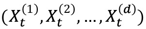 , then these terms are given by the following formula:

The higher order terms are given by iterated integrals of these component functions:

The full signature of a path is an infinite sequence – so for practical uses, we usually truncate at a particular depth that determines the maximum size of indices, such as ![]() here.
here.
This iterated integral definition is not especially useful in practice. Fortunately, when we sample a path and make the modest assumption that the path is linear between successive samples, then we can compute the signature by computing the product of tensor exponentials of increments. Concretely, if ![]() are sample values taken from our path
are sample values taken from our path ![]() at
at ![]() , respectively, all lying between
, respectively, all lying between ![]() and
and ![]() , then (assuming
, then (assuming ![]() is linear between
is linear between ![]() and
and ![]() ) the signature is given by the following:
) the signature is given by the following:

Here, the ![]() symbol denotes multiplication in the free tensor algebra (this multiplication is defined by the concatenation of indices – so, for instance, the
symbol denotes multiplication in the free tensor algebra (this multiplication is defined by the concatenation of indices – so, for instance, the ![]() -th value on the left and the
-th value on the left and the ![]() -th value on the right will contribute to the
-th value on the right will contribute to the ![]() -th value in the result). Remember that these are exponents of free tensor objects – not the usual exponential function – which are defined using the familiar power series:
-th value in the result). Remember that these are exponents of free tensor objects – not the usual exponential function – which are defined using the familiar power series:

When the constant term of a tensor ![]() is zero and we truncate the tensor algebra to depth
is zero and we truncate the tensor algebra to depth ![]() , then the value of
, then the value of ![]() is exactly equal to the sum of the first
is exactly equal to the sum of the first ![]() terms of this sum, which is a finite sum that can be computed efficiently.
terms of this sum, which is a finite sum that can be computed efficiently.
The importance of the signature of a path in a data science context is from the fact that the signature is representative of the path from the perspective of functions. Any continuous function defined on the path ![]() is approximately (in a very precise sense) a linear function defined on the signature. Thus, anything that can be learned about a path can also be learned from the signature.
is approximately (in a very precise sense) a linear function defined on the signature. Thus, anything that can be learned about a path can also be learned from the signature.
The esig package is built on top of the libalgebra C++ library for computations involving the free tensor algebra (and other kinds of algebraic objects). The stream2sig routine from esig takes a sequence of path samples in the form of an N (number of samples) x d (number of dimensions) NumPy array and returns a flat NumPy array containing the components of the signature, laid out in sequence as described here. The second argument to stream2sig is the depth parameter ![]() , which we have chosen to be 2 in this recipe. The size of the signature array is determined only by the dimension of the space and the depth, and is given by the following formula:
, which we have chosen to be 2 in this recipe. The size of the signature array is determined only by the dimension of the space and the depth, and is given by the following formula:
In the recipe, both of our paths were 2-dimensional, and signatures were computed to depth 2 so the signature has ![]() elements (notice that the number of samples varied in each case and were generated randomly and irregularly, yet the signature was the same size in each case).
elements (notice that the number of samples varied in each case and were generated randomly and irregularly, yet the signature was the same size in each case).
Now that the theory is out of the way, let’s look at the recipe. We define two true paths (signals), which we called signal a and signal b. We draw samples from each signal by drawing parameter values ![]() with differences taken from an exponential distribution so that (on average)
with differences taken from an exponential distribution so that (on average) ![]() . Then, we feed these parameter values into the formula for the path (see step 3). In the latter steps, we also add Gaussian noise to generated paths with mean 0 and variance 0.1. This guarantees that our 2 signals are irregularly sampled and noisy – to demonstrate the robustness of signature calculations.
. Then, we feed these parameter values into the formula for the path (see step 3). In the latter steps, we also add Gaussian noise to generated paths with mean 0 and variance 0.1. This guarantees that our 2 signals are irregularly sampled and noisy – to demonstrate the robustness of signature calculations.
Signal a is defined by the following formula:

Because this is a nice (smooth) path over the interval ![]() , we can compute the signature precisely using the iterated integrals to (approximately) get the sequence:
, we can compute the signature precisely using the iterated integrals to (approximately) get the sequence:
![]()
This is remarkably close to the computed signature for the signal as given here:
[1. 0.11204198 -0.95648657 0.0062767 -0.15236199 0.04519534 0.45743328]
We expect a reasonable amount of error because our sampling is fairly coarse (only 100 points) and our parameter values might finish before ![]() because of the way we randomized.
because of the way we randomized.
Signal b is defined by the following formula:
![]()
The component functions for this signal are also smooth, so we can compute the signature by computing the iterated integrals. Following this procedure, we see that the signature of the true signal is the following:
![]()
Comparing this to the compute value, we see that we’re fairly close:
[ 1.00000000e+00 7.19079669e-04 -3.23775977e-02 2.58537785e-07 3.12414826e+00 -3.12417155e+00 5.24154417e-04]
Again, we expect some error because of coarse sampling and not covering the parameter interval exactly (in Figure 7.16, you can see that there are some substantial “straight sections” indicating that the parameter values are spaced far apart in some places on the plots for signal b).
In step 6, we generate a number of signatures for noisy samples taken from both signals, all with different and irregular time steps (the count of which is also randomly drawn between 50 and 100) and Gaussian noise. These are stacked into an array with N = 50 rows and 7 columns (the size of the signature). We compute the row-wise mean of each array of signatures using the np.mean routine with axis=0. This produces an expected signature for each signal. We then compare these expected signatures to the “true signature” computed in step 5 and one another. We can see that the difference between the two expected signatures is significantly larger (not in the statistical sense) than the difference between the expected and true signatures for each signal. This illustrates the discriminative power of the signature for classifying time series data.
There’s more…
The example problem we addressed in the recipe is extremely simple. Signatures have been used in a wide variety of contexts, including sepsis detection, handwriting recognition, natural language processing, human action recognition, and drone identification. Usually, signatures are used in tandem with a selection of “preprocessing steps” that address various deficiencies in the sampled data. For example, in the recipe, we deliberately chose signals that are bounded (and relatively small) on the interval in question. In practice, data will likely be spread more widely and in this case, the higher order terms in the signature can grow quite rapidly, which can have important consequences for numerical stability. These preprocessing steps include lead-lag transformations, pen-on-pen-off transformations, the missing data transformation, and time integration. Each of these has a specific role in making data more amenable to signature based methods.
Signatures contain a large amount of redundancy. Many of the higher order terms can be computed from the others because of the geometry. This means that we can reduce the number of terms we need without discarding any information about the path. This reduction involves projecting the signature (in the free tensor algebra) onto the log signature (in the free Lie algebra). The log signature is an alternative representation of the path that has fewer terms than the signature. Many of the properties remain true for log signatures, except that we lose linearity in the approximation of functions (this may or may not be important for specific applications).
See also
The theory of rough paths and signature methods is obviously too broad – and rapidly expanding – to cover in such a short space. Here are some sources where you can find additional information about signatures:
- Lyons, T. and McLeod, A., 2022. Signature Methods in Machine Learning https://arxiv.org/abs/2206.14674
- Lyons, T., Caruana, M., and Lévy, T., 2004. Differential Equations Driven by Rough Paths, Springer, Ecole d’Eté de Probabilités de Saint-Flour XXXIV
- Several Jupyter notebooks walking through analyzing time series data using signatures on the Datasig website: https://datasig.ac.uk/examples.
Further reading
A good textbook on regression in statistics is the book Probability and Statistics by Mendenhall, Beaver, and Beaver, as mentioned in Chapter 6, Working with Data and Statistics. The following books provide a good introduction to classification and regression in modern data science:
- James, G. and Witten, D., 2013. An Introduction To Statistical Learning: With Applications In R. New York: Springer.
- Müller, A. and Guido, S., 2016. Introduction To Machine Learning With Python. Sebastopol: O’Reilly Media.
A good introduction to time series analysis can be found in the following book:
- Cryer, J. and Chan, K., 2008. Time Series Analysis. New York: Springer.