3

Calculus and Differential Equations

In this chapter, we will discuss various topics related to calculus. Calculus is the branch of mathematics that concerns the processes of differentiation and integration. Geometrically, the derivative of a function represents the gradient of the curve of the function, and the integral of a function represents the area below the curve of the function. Of course, these characterizations only hold in certain circumstances, but they provide a reasonable foundation for this chapter.

We’ll start by looking at calculus for a simple class of functions: polynomials. In the first recipe, we’ll create a class that represents a polynomial and define methods that differentiate and integrate the polynomial. Polynomials are convenient because the derivative or integral of a polynomial is again a polynomial. Then, we’ll use the SymPy package to perform symbolic differentiation and integration on more general functions. After that, we’ll look at methods for solving equations using the SciPy package. Then, we’ll turn our attention to numerical integration (quadrature) and solving differential equations. We’ll use the SciPy package to solve ordinary differential equations (ODEs) and systems of ODEs, and then use a finite difference scheme to solve a simple partial differential equation. Finally, we’ll use the Fast Fourier transform (FFT) to process a noisy signal and filter out the noise.

The content of this chapter will help you solve problems that involve calculus, such as computing the solution to differential equations, which frequently arise when describing the physical world. We’ll also dip into calculus later in Chapter 9 when we discuss optimization. Several optimization algorithms require some kind of knowledge of derivatives, including the backpropagation commonly used in machine learning (ML).

In this chapter, we will cover the following recipes:

• Working with polynomials and calculus
• Differentiating and integrating symbolically using SymPy
• Solving equations
• Integrating functions numerically using SciPy
• Solving simple differential equations numerically
• Solving systems of differential equations
• Solving partial differential equations numerically
• Using discrete Fourier transforms for signal processing
• Automatic differentiation and calculus using JAX
• Solving differential equations using JAX

Technical requirements

In addition to the scientific Python packages NumPy and SciPy, we also need the SymPy, JAX, and diffrax packages. These can be installed using your favorite package manager, such as pip:

python3.10 -m pip install sympy jaxlib jax sympy diffrax

There are different options for the way you install JAX. Please see the official documentation for more details: https://github.com/google/jax#installation.

The code for this chapter can be found in the Chapter 03 folder of the GitHub repository at https://github.com/PacktPublishing/Applying-Math-with-Python-2nd-Edition/tree/main/Chapter%2003.

Primer on calculus

Calculus is the study of functions and the way that they change. There are two major processes in calculus: differentiation and integration. Differentiation takes a function and produces a new function—called the derivative—that is the best linear approximation at each point. (You may see this described as the gradient of the function. Integration is often described as anti-differentiation—indeed, differentiating the integral of a function does give back the original function—but is also an abstract description of the area between the graph of the function and the axis, taking into account where the curve is above or below the axis.

Abstractly, the derivative of a function at a point is defined as a limit (which we won’t describe here) of the quantity:

This is because this small number becomes smaller and smaller. This is the difference in divided by the difference in , which is why the derivative is sometimes written as follows:

There are numerous rules for differentiating common function forms: for example, in the first recipe, we will see that the derivative of is . The derivative of the exponential function is, again, ; the derivative of is ; and the derivative of is . These basic building blocks can be combined using the product rule and chain rule, and by the fact that derivatives of sums are sums of derivatives, to differentiate more complex functions.

In its indefinite form, integration is the opposite process of differentiation. In its definite form, the integral of a function is the (signed) area that lies between the curve of and the axis—note that this is a simple number, not a function. The indefinite integral of is usually written like this:

Here, the derivative of this function is . The definite integral of between and is given by the following equation:

Here, is the indefinite integral of . We can, of course, define the indefinite integral abstractly, using limits of sums approximating the area below the curve, and then define the indefinite integral in terms of this abstract quantity. (We won’t go into detail here.) The most important thing to remember with indefinite integrals is the constant of integration.

There are several easily deduced indefinite integrals (anti-derivatives) that we can quickly deduce: the integral of is 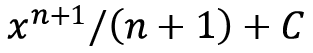(this is what we would differentiate to get ); the integral of is ; the integral of is ; and the integral of is . In all these examples, is the constant of integration. We can combine these simple rules to integrate more interesting functions by using the techniques of integration by parts or integration by substitution (and a host of much more involved techniques that we won’t mention here).

Working with polynomials and calculus

Polynomials are among the simplest functions in mathematics and are defined as a sum:

Here, represents a placeholder to be substituted (an indeterminate), and is a number. Since polynomials are simple, they provide an excellent means for a brief introduction to calculus.

In this recipe, we will define a simple class that represents a polynomial and write methods for this class to perform differentiation and integration.

Getting ready

There are no additional packages required for this recipe.

How to do it...

The following steps describe how to create a class representing a polynomial, and implement differentiation and integration methods for this class:

1. Let’s start by defining a simple class to represent a polynomial:

   class Polynomial:

       """Basic polynomial class"""

       def __init__(self, coeffs):

          self.coeffs = coeffs

       def __repr__(self):

          return f"Polynomial({repr(self.coeffs)})"

       def __call__(self, x):

         return sum(coeff*x**i for i, coeff in enumerate(    	        self.coeffs))
2. Now that we have defined a basic class for a polynomial, we can move on to implement the differentiation and integration operations for this Polynomial class to illustrate how these operations change polynomials. We start with differentiation. We generate new coefficients by multiplying each element in the current list of coefficients without the first element. We use this new list of coefficients to create a new Polynomial instance that is returned:

       def differentiate(self):

         """Differentiate the polynomial and return the derivative"""

           coeffs = [i*c for i, c in enumerate(

               self.coeffs[1:], start=1)]

           return Polynomial(coeffs)
3. To implement the integration method, we need to create a new list of coefficients containing the new constant (converted to a float for consistency) given by the argument. We then add to this list of coefficients the old coefficients divided by their new position in the list:

       def integrate(self, constant=0):

         """Integrate the polynomial and return the integral"""

           coeffs = [float(constant)]

           coeffs += [c/i for i, c in enumerate(

               self.coeffs, start=1)]

           return Polynomial(coeffs)
4. Finally, to make sure these methods work as expected, we should test these two methods with a simple case. We can check this using a very simple polynomial, such as :

   p = Polynomial([1, -2, 1])

   p.differentiate()

   # Polynomial([-2, 2])

   p.integrate(constant=1)

   # Polynomial([1.0, 1.0, -1.0, 0.3333333333])

The derivative here is given the coefficients and , which corresponds to the polynomial , which is indeed the derivative of . Similarly, the coefficients of the integral correspond to the polynomial , which is also correct (with constant of integration ).

How it works...

Polynomials offer an easy introduction to the basic operations of calculus, but it isn’t so easy to construct Python classes for other general classes of functions. That being said, polynomials are extremely useful because they are well understood and, perhaps more importantly, calculus for polynomials is very easy. For powers of a variable , the rule for differentiation is to multiply by the power and reduce the power by 1 so that becomes , so our rule for differentiating a polynomial is to simply multiply each coefficient by its position and remove the first coefficient.

Integration is more complex since the integral of a function is not unique. We can add any constant to an integral and obtain a second integral. For powers of a variable , the rule for integration is to increase the power by 1 and divide by the new power so that becomes . Therefore, to integrate a polynomial, we increase each power of by 1 and divide the corresponding coefficient by the new power. Hence, our rule is to first insert the new constant of integration as the first element and divide each of the existing coefficients by its new position in the list.

The Polynomial class that we defined in the recipe is rather simplistic but represents the core idea. A polynomial is uniquely determined by its coefficients, which we can store as a list of numerical values. Differentiation and integration are operations that we can perform on this list of coefficients. We include a simple __repr__ method to help with the display of Polynomial objects, and a __call__ method to facilitate evaluation at specific numerical values. This is mostly to demonstrate the way that a polynomial is evaluated.

Polynomials are useful for solving certain problems that involve evaluating a computationally expensive function. For such problems, we can sometimes use some kind of polynomial interpolation, where we fit a polynomial to another function, and then use the properties of polynomials to help solve the original problem. Evaluating a polynomial is much cheaper than the original function, so this can lead to dramatic improvements in speed. This usually comes at the cost of some accuracy. For example, Simpson’s rule for approximating the area under a curve approximates the curve by quadratic polynomials over intervals defined by three consecutive mesh points. The area below each quadratic polynomial can be calculated easily by integration.

There’s more...

Polynomials have many more important roles in computational programming than simply demonstrating the effect of differentiation and integration. For this reason, a much richer Polynomial class is provided in the numpy.polynomial NumPy package. The NumPy Polynomial class, and the various derived subclasses, are useful in all kinds of numerical problems and support arithmetic operations as well as other methods. In particular, there are methods for fitting polynomials to collections of data.

NumPy also provides classes, derived from Polynomial, that represent various special kinds of polynomials. For example, the Legendre class represents a specific system of polynomials called Legendre polynomials. Legendre polynomials are defined for satisfying and form an orthogonal system, which is important for applications such as numerical integration and the finite element method for solving partial differential equations. Legendre polynomials are defined using a recursive relation. We define them as follows:

Furthermore, for each , we define the th Legendre polynomial to satisfy the recurrence relation:

There are several other so-called orthogonal (systems of) polynomials, including Laguerre polynomials, Chebyshev polynomials, and Hermite polynomials.

See also

Calculus is certainly well documented in mathematical texts, and there are many textbooks that cover the basic methods all the way to the deep theory. Orthogonal systems of polynomials are also well documented among numerical analysis texts.

Differentiating and integrating symbolically using SymPy

At some point, you may have to differentiate a function that is not a simple polynomial, and you may need to do this in some kind of automated fashion—for example, if you are writing software for education. The Python scientific stack includes a package called SymPy, which allows us to create and manipulate symbolic mathematical expressions within Python. In particular, SymPy can perform differentiation and integration of symbolic functions, just like a mathematician.

In this recipe, we will create a symbolic function and then differentiate and integrate this function using the SymPy library.

Getting ready

Unlike some of the other scientific Python packages, there does not seem to be a standard alias under which SymPy is imported in the literature. Instead, the documentation uses a star import at several points, which is not in line with the PEP8 style guide. This is possibly to make the mathematical expressions more natural. We will simply import the module under its name sympy, to avoid any confusion with the scipy package’s standard abbreviation, sp (which is the natural choice for sympy too):

import sympy

In this recipe, we will define a symbolic expression that represents the following function:

Then, we will see how to symbolically differentiate and integrate this function.

How to do it...

Differentiating and integrating symbolically (as you would do by hand) is very easy using the SymPy package. Follow these steps to see how it is done:

1. Once SymPy is imported, we define the symbols that will appear in our expressions. This is a Python object that has no particular value, just like a mathematical variable, but can be used in formulas and expressions to represent many different values simultaneously. For this recipe, we need only define a symbol for , since we will only require constant (literal) symbols and functions in addition to this. We use the symbols routine from sympy to define a new symbol. To keep the notation simple, we will name this new symbol x:

   x = sympy.symbols('x')
2. The symbols defined using the symbols function support all of the arithmetic operations, so we can construct the expression directly using the symbol x we just defined:

   f = (x**2 - 2*x)*sympy.exp(3 - x)
3. Now, we can use the symbolic calculus capabilities of SymPy to compute the derivative of f—that is, differentiate f. We do this using the diff routine in sympy, which differentiates a symbolic expression with respect to a specified symbol and returns an expression for the derivative. This is often not expressed in its simplest form, so we use the sympy.simplify routine to simplify the result:

   fp = sympy.simplify(sympy.diff(f))

   print(fp)  # (-x**2 + 4*x - 2)*exp(3 - x)
4. We can check whether the result of the symbolic differentiation using SymPy is correct, compared to the derivative computed by hand using the product rule, defined as a SymPy expression, as follows:

   fp2 = (2*x - 2)*sympy.exp(3 - x) - (

       x**2 - 2*x)*sympy.exp(3 - x)
5. SymPy equality tests whether two expressions are equal, but not whether they are symbolically equivalent. Therefore, we must first simplify the difference of the two statements we wish to test and test for equality to 0:

   print(sympy.simplify(fp2 - fp) == 0)  # True
6. We can integrate the derivative fp using SymPy by using the integrate function and check that this is again equal to f. It is a good idea to also provide the symbol with which the integration is to be performed by providing it as the second optional argument:

   F = sympy.integrate(fp, x)

   print(F)  # (x**2 - 2*x)*exp(3 - x)

As we can see, the result of integrating the derivative fp gives back the original function f (although we are technically missing the constant of integration ).

How it works...

SymPy defines various classes to represent certain kinds of expressions. For example, symbols, represented by the Symbol class, are examples of atomic expressions. Expressions are built up in a similar way to how Python builds an abstract syntax tree from source code. These expression objects can then be manipulated using methods and standard arithmetic operations.

SymPy also defines standard mathematical functions that can operate on Symbol objects to create symbolic expressions. The most important feature is the ability to perform symbolic calculus—rather than the numerical calculus that we explore in the remainder of this chapter—and give exact (sometimes called analytic) solutions to calculus problems.

The diff routine from the SymPy package performs differentiation on these symbolic expressions. The result of this routine is usually not in its simplest form, which is why we used the simplify routine to simplify the derivative in the recipe. The integrate routine symbolically integrates a scipy expression with respect to a given symbol. (The diff routine also accepts a symbol argument that specifies the symbol for differentiating against.) This returns an expression whose derivative is the original expression. This routine does not add a constant of integration, which is good practice when doing integrals by hand.

There’s more...

SymPy can do much more than simple algebra and calculus. There are submodules for various areas of mathematics, such as number theory, geometry, and other discrete mathematics (such as combinatorics).

SymPy expressions (and functions) can be built into Python functions that can be applied to NumPy arrays. This is done using the lambdify routine from the sympy.utilities module. This converts a SymPy expression to a numerical expression that uses the NumPy equivalents of the SymPy standard functions to evaluate the expressions numerically. The result is similar to defining a Python Lambda, hence the name. For example, we could convert the function and derivative from this recipe into Python functions using this routine:

from sympy.utilities import lambdify
lam_f = lambdify(x, f)
lam_fp = lambdify(x, fp)

The lambdify routine takes two arguments. The first is the variables to be provided, x in the previous code block, and the second is the expression to be evaluated when this function is called. For example, we can evaluate the lambdified SymPy expressions defined previously as if they were ordinary Python functions:

lam_f(4)  # 2.9430355293715387
lam_fp(7)  # -0.4212596944408861

We can even evaluate these lambdified expressions on NumPy arrays (as usual, with NumPy imported as np):

lam_f(np.array([0, 1, 2]))  # array([ 0. , -7.3890561, 0. ])

Note

The lambdify routine uses the Python exec routine to execute the code, so it should not be used with unsanitized input.

Solving equations

Many mathematical problems eventually reduce to solving an equation of the form , where is a function of a single variable. Here, we try to find a value of for which the equation holds. The values of for which the equation holds are sometimes called roots of the equation. There are numerous algorithms for finding solutions to equations of this form. In this recipe, we will use the Newton-Raphson and secant methods to solve an equation of the form .

The Newton-Raphson method (Newton’s method) and the secant method are good, standard root-finding algorithms that can be applied in almost any situation. These are iterative methods that start with an approximation of the root and iteratively improve this approximation until it lies within a given tolerance.

To demonstrate these techniques, we will use the function from the Differentiating and integrating symbolically using SymPy recipe, defined by the following formula:

This is defined for all real values of and has exactly two roots, one at and one at .

Getting ready

The SciPy package contains routines for solving equations (among many other things). The root-finding routines can be found in the optimize module from the scipy package. As usual, we import NumPy as np.

How to do it...

The optimize package provides routines for numerical root finding. The following instructions describe how to use the newton routine from this module:

1. The optimize module is not listed in the scipy namespace, so you must import it separately:

   from scipy import optimize
2. Then, we must define this function and its derivative in Python:

   from math import exp

   def f(x):

     return x*(x - 2)*exp(3 - x)
3. The derivative of this function was computed in the previous recipe:

   def fp(x):

     return -(x**2 - 4*x + 2)*exp(3 - x)
4. For both the Newton-Raphson and secant methods, we use the newton routine from optimize. Both the secant method and the Newton-Raphson method require the function as the first argument and the first approximation, x0, as the second argument. To use the Newton-Raphson method, we must provide the derivative of , using the fprime keyword argument:

   optimize.newton(f, 1, fprime=fp) # Using the Newton-Raphson method

   # 2.0
5. To use the secant method, only the function is needed, but we must provide the first two approximations for the root; the second is provided as the x1 keyword argument:

   optimize.newton(f, 1., x1=1.5) # Using x1 = 1.5 and the secant method

   # 1.9999999999999862

Note

Neither the Newton-Raphson nor the secant method is guaranteed to converge to a root. It is perfectly possible that the iterates of the method will simply cycle through a number of points (periodicity) or fluctuate wildly (chaos).

How it works...

The Newton-Raphson method for a function with derivative and initial approximation is defined iteratively using this formula:

For each integer, . Geometrically, this formula arises by considering the direction in which the gradient is negative (so, the function is decreasing) if or positive (so, the function is increasing) if .

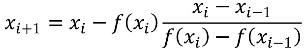
The secant method is based on the Newton-Raphson method, but replaces the first derivative with the following approximation:

When is sufficiently small, which occurs if the method is converging, then this is a good approximation. The price paid for not requiring the derivative of the function is that we require an additional initial guess to start the method. The formula for the method is given as follows:

Generally speaking, if either method is given an initial guess (guesses for the secant method) that is sufficiently close to a root, then the method will converge to that root. The Newton-Raphson method can also fail if the derivative is zero at one of the iterations, in which case the formula is not well defined.

There’s more...

The methods mentioned in this recipe are general-purpose methods, but there are others that may be faster or more accurate in some circumstances. Broadly speaking, root-finding algorithms fall into two categories: algorithms that use information about the function’s gradient at each iterate (Newton-Raphson, secant, Halley) and algorithms that require bounds on the location of a root (bisection method, Regula-Falsi, Brent). The algorithms discussed so far are of the first kind, and while generally quite fast, they may fail to converge.

The second kind of algorithm is those for which a root is known to exist within a specified interval . We can check whether a root lies within such an interval by checking that and have different signs—that is, one of or is true (provided, of course, that the function is continuous, which tends to be the case in practice). The most basic algorithm of this kind is the bisection algorithm, which repeatedly bisects the interval until a sufficiently good approximation to the root is found. The basic premise is to split the interval between and at the mid-point and select the interval in which the function changes sign. The algorithm repeats until the interval is very small. The following is a rudimentary implementation of this algorithm in Python:

from math import copysign
def bisect(f, a, b, tol=1e-5):
    """Bisection method for root finding"""
    fa, fb = f(a), f(b)
    assert not copysign(fa, fb) == fa, "Function must change signs"
    while (b - a) > tol:
        m = (a + b)/2 # mid point of the interval
        fm = f(m)
        if fm == 0:
            return m
        if copysign(fm, fa) == fm: # fa and fm have the same sign
            a = m
            fa = fm
        else: # fb and fm have the same sign
            b = m
    return a

This method is guaranteed to converge since, at each step, the distance is halved. However, it is possible that the method will require more iterations than Newton-Raphson or the secant method. A version of the bisection method can also be found in optimize. This version is implemented in C and is considerably more efficient than the version presented here, but the bisection method is not the fastest method in most cases.

Brent’s method is an improvement on the bisection method and is available in the optimize module as brentq. It uses a combination of bisection and interpolation to quickly find the root of an equation:

optimize.brentq(f, 1.0, 3.0)  # 1.9999999999998792

It is important to note that the techniques that involve bracketing (bisection, regula-falsi, Brent) cannot be used to find the root functions of a complex variable, whereas those techniques that do not use bracketing (Newton, secant, Halley) can.

Finally, some equations are not quite of the form but can still be solved using these techniques. This is done by rearranging the equation so that it is of the required form (renaming functions if necessary). This is usually not too difficult and simply requires moving any terms on the right-hand side over to the left-hand side. For example, if you wish to find the fixed points of a function—that is, when —then we would apply the method to the related function given by .

Integrating functions numerically using SciPy

Integration can be interpreted as the area that lies between a curve and the axis, signed according to whether this area is above or below the axis. Some integrals cannot be computed directly using symbolic means, and instead, have to be approximated numerically. One classic example of this is the Gaussian error function, which was mentioned in the Understanding basic mathematical functions section in Chapter 1, An Introduction to Basic Packages, Functions, and Concepts. This is defined by the following formula:

Furthermore, the integral that appears here cannot be evaluated symbolically.

In this recipe, we will see how to use numerical integration routines in the SciPy package to compute the integral of a function.

Getting ready

We use the scipy.integrate module, which contains several routines for computing numerical integrals. We also import the NumPy library as np. We import this module as follows:

from scipy import integrate

How to do it...

The following steps describe how to numerically integrate a function using SciPy:

1. We evaluate the integral that appears in the definition of the error function at the value . For this, we need to define the integrand (the function that appears inside the integral) in Python:

   def erf_integrand(t):

       return np.exp(-t**2)

There are two main routines in scipy.integrate for performing numerical integration (quadrature) that can be used. The first is the quad function, which uses QUADPACK to perform the integration, and the second is quadrature.

2. The quad routine is a general-purpose integration tool. It expects three arguments, which are the function to be integrated (erf_integrand), the lower limit (-1.0), and the upper limit (1.0):

   val_quad, err_quad = integrate.quad(erf_integrand, -1.0, 1.0)

   # (1.493648265624854, 1.6582826951881447e-14)

The first returned value is the value of the integral, and the second is an estimate of the error.

3. Repeating the computation with the quadrature routine, we get the following. The arguments are the same as for the quad routine:

   val_quadr, err_quadr =

       integrate.quadrature(

           erf_integrand, -1.0, 1.0)

   # (1.4936482656450039, 7.459897144457273e-10)

The output is the same format as the code, with the value of the integral and then an estimate of the error. Notice that the error is larger for the quadrature routine. This is a result of the method terminating once the estimated error falls below a given tolerance, which can be modified when the routine is called.

How it works...

Most numerical integration techniques follow the same basic procedure. First, we choose points for in the region of integration, and then use these values and the values to approximate the integral. For example, with the trapezium rule, we approximate the integral with the following formula:

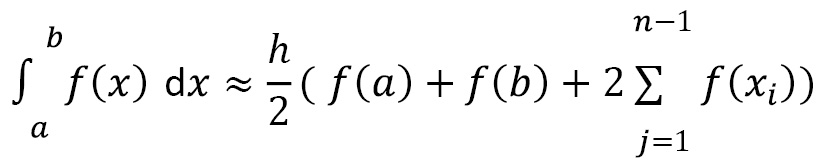
Here, and is the (common) difference between adjacent values, including the endpoints and . This can be implemented in Python as follows:

def trapezium(func, a, b, n_steps):
    """Estimate an integral using the trapezium rule"""
    h = (b - a) / n_steps
    x_vals = np.arange(a + h, b, h) 
    y_vals = func(x_vals)
    return 0.5*h*(func(a) + func(b) + 2.*np.sum(y_vals))

The algorithms used by quad and quadrature are far more sophisticated than this. Using this function to approximate the integral of erf_integrand using trapezium with 500 steps yields a result of 1.4936463036001209, which agrees with the approximations from the quad and quadrature routines to five decimal places.

The quadrature routine uses a fixed tolerance Gaussian quadrature, whereas the quad routine uses an adaptive algorithm implemented in the Fortran library QUADPACK routines. Timing both routines, we find that the quad routine is approximately five times faster than the quadrature routine for the problem described in the recipe. The quad routine executes in approximately 27 µs, averaging over 1 million executions, while the quadrature routine executes in approximately 134 µs. (Your results may differ depending on your system.) Generally speaking, you should use the quad method since it is both faster and more accurate unless you need the Gaussian quadrature implemented by quadrature.

There’s more...

The routines mentioned in this section require the integrand function to be known, which is not always the case. Instead, it might be the case that we know a number of pairs with , but we don’t know the function to evaluate at additional points. In this case, we can use one of the sampling quadrature techniques from scipy.integrate. If the number of known points is very large and all points are equally spaced, we can use Romberg integration for a good approximation of the integral. For this, we use the romb routine. Otherwise, we can use a variant of the trapezium rule (as shown previously) using the trapz routine, or Simpson’s rule using the simps routine.

Solving simple differential equations numerically

Differential equations arise in situations where a quantity evolves, usually over time, according to a given relationship. They are extremely common in engineering and physics, and appear quite naturally. One of the classic examples of a (very simple) differential equation is the law of cooling devised by Newton. The temperature of a body cools at a rate proportional to the current temperature. Mathematically, this means that we can write the derivative of the temperature of the body at time using the following differential equation:

Here, is a positive constant that determines the rate of cooling. This differential equation can be solved analytically by first separating the variables and then integrating and rearranging them. After performing this procedure, we obtain the general solution:

Here, is the initial temperature.

In this recipe, we will solve a simple ODE numerically using the solve_ivp routine from SciPy.

Getting ready

We will demonstrate the technique for solving a differential equation numerically in Python using the cooling equation described previously since we can compute the true solution in this case. We take the initial temperature to be and . Let’s also find the solution for values between and .

For this recipe, we will need the NumPy library imported as np, the Matplotlib pyplot interface imported as plt, and the integrate module imported from SciPy:

from scipy import integrate

A general (first-order) differential equation has the following form:

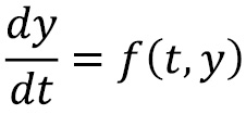
Here, is some function of (the independent variable) and (the dependent variable). In this formula, is the dependent variable and . The routines for solving differential equations in the SciPy package require the function and an initial value and the range of values where we need to compute the solution. To get started, we need to define our function in Python and create a variables and range ready to be supplied to the SciPy routine:

def f(t, y):
    return -0.2*y
t_range = (0, 5)

Next, we need to define the initial condition from which the solution should be found. For technical reasons, the initial values must be specified as a one-dimensional NumPy array:

T0 = np.array([50.])

Since, in this case, we already know the true solution, we can also define this in Python ready to compare to the numerical solution that we will compute:

def true_solution(t):
    return 50.*np.exp(-0.2*t)

Let’s see how to solve this initial value problem using SciPy.

How to do it...

Follow these steps to solve a differential equation numerically and plot the solution along with the error:

1. We use the solve_ivp routine from the integrate module in SciPy to solve the differential equation numerically. We add a parameter for the maximum step size, with a value of 0.1, so that the solution is computed at a reasonable number of points:

   sol = integrate.solve_ivp(f, t_range, T0, max_step=0.1)
2. Next, we extract the solution values from the sol object returned from the solve_ivp method:

   t_vals = sol.t

   T_vals = sol.y[0, :]
3. Next, we plot the solution on a set of axes, as follows. Since we are also going to plot the approximation error on the same figure, we create two subplots using the subplots routine:

   fig, (ax1, ax2) = plt.subplots(1, 2, tight_layout=True)

   ax1.plot(t_vals, T_valsm "k")

   ax1.set_xlabel("$t$")

   ax1.set_ylabel("$T$")

   ax1.set_title("Solution of the cooling equation")

This plots the solution on a set of axes displayed on the left-hand side of Figure 3.1.

4. To do this, we need to compute the true solution at the points that we obtained from the solve_ivp routine, and then calculate the absolute value of the difference between the true and approximated solutions:

   err = np.abs(T_vals - true_solution(t_vals))
5. Finally, on the right-hand side of Figure 3.1, we plot the error in the approximation with a logarithmic scale on the axis. We can then plot this on the right-hand side with a logarithmic scale axis using the semilogy plot command, as we saw in Chapter 2, Mathematical Plotting with Matplotlib:

   ax2.semilogy(t_vals, err, "k")

   ax2.set_xlabel("$t$")

   ax2.set_ylabel("Error")

   ax2.set_title("Error in approximation")

The left-hand plot in Figure 3.1 shows decreasing temperature over time, while the right-hand plot shows that the error increases as we move away from the known value given by the initial condition:

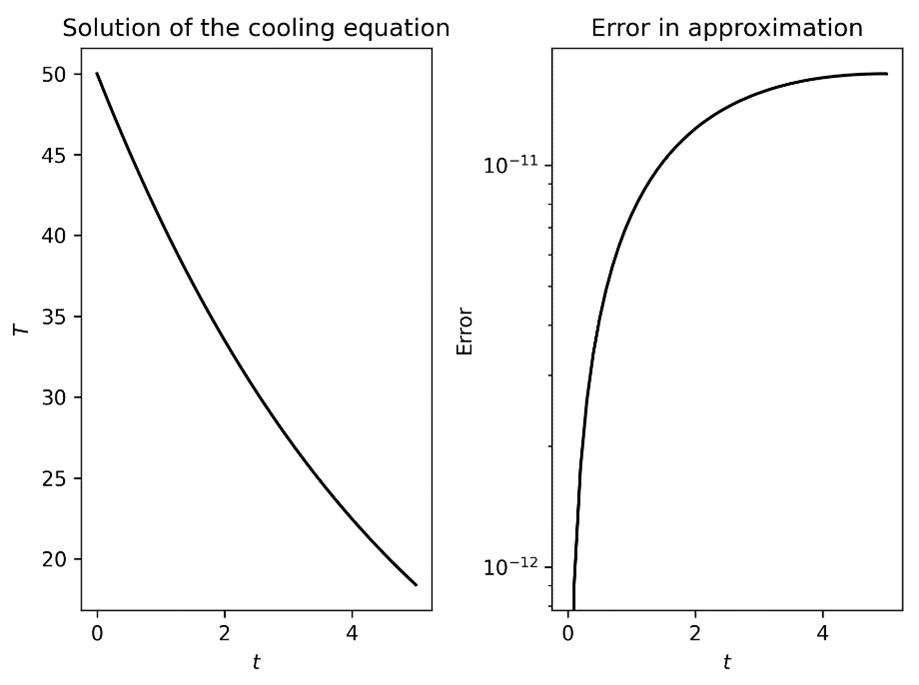
Figure 3.1 – Plot of the numerical solution to the cooling equation

Notice that the right-hand side plot is on a logarithmic scale and, while the rate of increase looks fairly dramatic, the values involved are very small (of order ).

How it works...

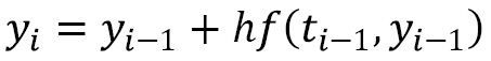
Most methods for solving differential equations are time-stepping methods. The pairs are generated by taking small steps and approximating the value of the function . This is perhaps best illustrated by Euler’s method, which is the most basic time-stepping method. Fixing a small step size , we form the approximation at the th step using the following formula:

We start from the known initial value . We can easily write a Python routine that performs Euler’s method as follows (there are, of course, many different ways to implement Euler’s method; this is a very simple example).

First, we set up the method by creating lists that will store the values and values that we will return:

def euler(func, t_range, y0, step_size):
    """Solve a differential equation using Euler's method"""
    t = [t_range[0]]
    y = [y0]
    i = 0

Euler’s method continues until we hit the end of the range. Here, we use a while loop to accomplish this. The body of the loop is very simple; we first increment a counter i, and then append the new and values to their respective lists:

    while t[i] < t_range[1]:
        i += 1
        t.append(t[i-1] + step_size)  # step t
        y.append(y[i-1] + step_size*func(
           t[i-1], y[i-1]))   # step y
    return t, y

The method used by the solve_ivp routine, by default, is the Runge-Kutta-Fehlberg (RKF45) method, which has the ability to adapt the step size to ensure that the error in the approximation stays within a given tolerance. This routine expects three positional arguments: the function , the range on which the solution should be found, and the initial value ( in our example). Optional arguments can be provided to change the solver, the number of points to compute, and several other settings.

The function passed to the solve_ivp routine must have two arguments, as in the general differential equation described in the Getting ready section. The function can have additional arguments, which can be provided using the args keyword for the solve_ivp routine, but these must be positioned after the two necessary arguments. Comparing the euler routine we defined earlier to the solve_ivp routine, both with a (maximum) step size of 0.1, we find that the maximum true error between the solve_ivp solution is in the order of 10-11, whereas the euler solution only manages an error of 0.19. The euler routine is working, but the step size is much too large to overcome the accumulating error. For comparison, Figure 3.2 is a plot of the solution and error as produced by Euler’s method. Compare Figure 3.2 to Figure 3.1. Note the scale on the error plot is dramatically different:

Figure 3.2 – Plot of solution and error using Euler’s method with step size 0.1

The solve_ivp routine returns a solution object that stores information about the solution that has been computed. Most important here are the t and y attributes, which contain the values on which the solution is computed and the solution itself. We used these values to plot the solution we computed. The values are stored in a NumPy array of shape (n, N), where n is the number of components of the equation (here, 1), and N is the number of points computed. The values held in sol are stored in a two-dimensional array, which in this case has one row and many columns. We use the slice y[0, :] to extract this first row as a one-dimensional array that can be used to plot the solution in step 4.

We use a logarithmically scaled axis to plot the error because what is interesting there is the order of magnitude. Plotting it on a non-scaled axis would give a line that is very close to the axis, which doesn’t show the increase in the error as we move through the values. The logarithmically scaled axis shows this increase clearly.

There’s more...

The solve_ivp routine is a convenient interface for a number of solvers for differential equations, the default being the RKF45 method. The different solvers have different strengths, but the RKF45 method is a good general-purpose solver.

See also

For more detailed instructions on how to add subplots to a figure in Matplotlib, see the Adding subplots recipe from Chapter 2, Mathematical Plotting with Matplotlib.

Solving systems of differential equations

Differential equations sometimes occur in systems consisting of two or more interlinked differential equations. A classic example is a simple model of the populations of competing species. This is a simple model of competing species labeled (the prey) and (the predators) given by the following equations:

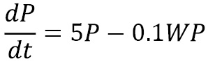
The first equation dictates the growth of the prey species , which, without any predators, would be exponential growth. The second equation dictates the growth of the predator species , which, without any prey, would be exponential decay. Of course, these two equations are coupled; each population change depends on both populations. The predators consume the prey at a rate proportional to the product of their two populations, and the predators grow at a rate proportional to the relative abundance of prey (again the product of the two populations).

In this recipe, we will analyze a simple system of differential equations and use the SciPy integrate module to obtain approximate solutions.

Getting ready

The tools for solving a system of differential equations using Python are the same as those for solving a single equation. We again use the solve_ivp routine from the integrate module in SciPy. However, this will only give us a predicted evolution over time with given starting populations. For this reason, we will also employ some plotting tools from Matplotlib to better understand the evolution. As usual, the NumPy library is imported as np and the Matplotlib pyplot interface is imported as plt.

How to do it...

The following steps walk us through how to analyze a simple system of differential equations:

1. Our first task is to define a function that holds the system of equations. This function needs to take two arguments as for a single equation, except the dependent variable (in the notation from the Solving simple differential equations numerically recipe) will now be an array with as many elements as there are equations. Here, there will be two elements. The function we need for the example system in this recipe is defined as follows:

   def predator_prey_system(t, y):

       return np.array([5*y[0] - 0.1*y[0]*y[1],

           0.1*y[1]*y[0] - 6*y[1]])
2. Now we have defined the system in Python, we can use the quiver routine from Matplotlib to produce a plot that will describe how the populations will evolve—given by the equations—at numerous starting populations. We first set up a grid of points on which we will plot this evolution. It is a good idea to choose a relatively small number of points for the quiver routine; otherwise, it becomes difficult to see details in the plot. For this example, we plot the population values between 0 and 100:

   p = np.linspace(0, 100, 25)

   w = np.linspace(0, 100, 25)

   P, W = np.meshgrid(p, w)
3. Now, we compute the values of the system at each of these pairs. Notice that neither equation in the system is time-dependent (they are autonomous); the time variable is unimportant in the calculation. We supply the value 0 for the argument:

   dp, dw = predator_prey_system(0, np.array([P, W]))
4. The dp and dw variables now hold the direction in which the population of and will evolve, respectively, if we started at each point in our grid. We can plot these directions together using the quiver routine from matplotlib.pyplot:

   fig, ax = plt.subplots()

   ax.quiver(P, W, dp, dw)

   ax.set_title("Population dynamics for two competing species")

   ax.set_xlabel("P")

   ax.set_ylabel("W")

Plotting the result of these commands now gives us Figure 3.3, which gives a global picture of how solutions evolve:

Figure 3.3 – A quiver plot showing the population dynamics of two competing species

To understand a solution more specifically, we need some initial conditions so that we can use the solve_ivp routine described in the previous recipe.

5. Since we have two equations, our initial conditions will have two values. (Recall in the Solving simple differential equations numerically recipe, we saw that the initial condition provided to solve_ivp needs to be a NumPy array.) Let’s consider the initial values and . We define these in a NumPy array, being careful to place them in the correct order:

   initial_conditions = np.array([85, 40])
6. Now, we can use solve_ivp from the scipy.integrate module. We need to provide the max_step keyword argument to make sure that we have enough points in the solution to give a smooth solution curve:

   from scipy import integrate

   t_range = (0.0, 5.0)

   sol = integrate.solve_ivp(predator_prey_system,

                             t_range,

                             initial_conditions,

                             max_step=0.01)
7. Let’s plot this solution on our existing figure to show how this specific solution relates to the direction plot we have already produced. We also plot the initial condition at the same time:

   ax.plot(initial_conditions[0],

       initial_conditions[1], "ko")

   ax.plot(sol.y[0, :], sol.y[1, :], "k", linewidth=0.5)

The result of this is shown in Figure 3.4:

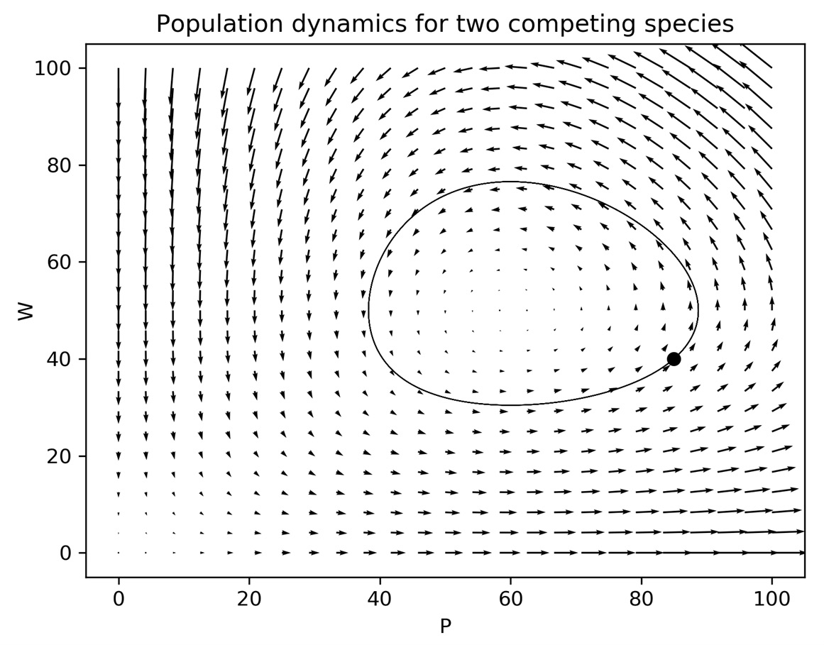
Figure 3.4 – Solution trajectory plotted over a quiver plot showing the general behavior

We can see that the trajectory plotted is a closed loop. This means that the populations have a stable and periodic relationship. This is a common pattern when solving these equations.

How it works...

The method used for a system of ODEs is exactly the same as for a single ODE. We start by writing the system of equations as a single vector differential equation:

This can then be solved using a time-stepping method as though were a simple scalar value.

The technique of plotting the directional arrows on a plane using the quiver routine is a quick and easy way of learning how a system might evolve from a given state. The derivative of a function represents the gradient of the curve , and so a differential equation describes the gradient of the solution function at position and time . A system of equations describes the gradient of separate solution functions at a given position and time . Of course, the position is now a two-dimensional point, so when we plot the gradient at a point, we represent this as an arrow that starts at the point, in the direction of the gradient. The length of the arrow represents the size of the gradient; the longer the arrow, the faster the solution curve will move in that direction.

When we plot the solution trajectory on top of this direction field, we can see that the curve (starting at the point) follows the direction indicated by the arrows. The behavior shown by the solution trajectory is a limit cycle, where the solution for each variable is periodic as the two species’ populations grow or decline. This description of the behavior is perhaps clearer if we plot each population against time, as seen in Figure 3.5. What is not immediately obvious from Figure 3.4 is that the solution trajectory loops around several times, but this is clearly shown in Figure 3.5:

Figure 3.5 – Plots of populations P and W against time

The periodic relationship described previously is clear in Figure 3.5. Moreover, we can see the lag between the peak populations of the two species. Species experiences peak population approximately 0.3 time periods after species .

There’s more...

The technique of analyzing a system of ODEs by plotting variables against one another, starting at various initial conditions, is called phase space (plane) analysis. In this recipe, we used the quiver plotting routine to quickly generate an approximation of the phase plane for a system of differential equations. By analyzing the phase plane of a system of differential equations, we can identify different local and global characteristics of the solution, such as limit cycles.

Solving partial differential equations numerically

Partial differential equations are differential equations that involve partial derivatives of functions in two or more variables, as opposed to ordinary derivatives in only a single variable. Partial differential equations are a vast topic, and could easily fill a series of books. A typical example of a partial differential equation is the (one-dimensional) heat equation:

Here, is a positive constant and is a function. The solution to this partial differential equation is a function , which represents the temperature of a rod, occupying the range , at a given time . To keep things simple, we will take , which amounts to saying that no heating/cooling is applied to the system, , and . In practice, we can rescale the problem to fix the constant , so this is not a restrictive problem. In this example, we will use boundary conditions:

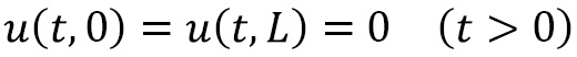
These are equivalent to saying that the ends of the rod are held at the constant temperature 0. We will also use the initial temperature profile:

This initial temperature profile describes a smooth curve between the values of 0 and 2 that peaks at a value of 3, which might be the result of heating the rod at the center to a temperature of 3.

We’re going to use a method called finite differences, where we divide the rod into a number of equal segments and the time range into a number of discrete steps. We then compute approximations for the solution at each of the segments and each time step.

In this recipe, we will use finite differences to solve a simple partial differential equation.

Getting ready

For this recipe, we will need the NumPy and Matplotlib packages, imported as np and plt, as usual. We also need to import the mplot3d module from mpl_toolkits since we will be producing a 3D plot:

from mpl_toolkits import mplot3d

We will also need some modules from the SciPy package.

How to do it...

In the following steps, we work through solving the heat equation using finite differences:

1. Let’s first create variables that represent the physical constraints of the system—the extent of the bar and the value of :

   alpha = 1

   x0 = 0 # Left hand x limit

   xL = 2 # Right hand x limit
2. We first divide the range into equal intervals—we take for this example—using points. We can use the linspace routine from NumPy to generate these points. We also need the common length of each interval :

   N = 10

   x = np.linspace(x0, xL, N+1)

   h = (xL - x0) / N
3. Next, we need to set up the steps in the time direction. We take a slightly different approach here; we set the time step size and the number of steps (implicitly making the assumption that we start at time 0):

   k = 0.01

   steps = 100

   t = np.array([i*k for i in range(steps+1)])
4. In order for the method to behave properly, we must have the following formula:
   

Otherwise, the system can become unstable. We store the left-hand side of this in a variable for use in step 5, and use an assertion to check that this inequality holds:

r = alpha*k / h**2
assert r < 0.5, f"Must have r < 0.5, currently r={r}"

5. Now, we can construct a matrix that holds the coefficients from the finite difference scheme. To do this, we use the diags routine from the scipy.sparse module to create a sparse, tridiagonal matrix:

   from scipy import sparse

   diag = [1, *(1-2*r for _ in range(N-1)), 1]

   abv_diag = [0, *(r for _ in range(N-1))]

   blw_diag = [*(r for _ in range(N-1)), 0]

   A = sparse.diags([blw_diag, diag, abv_diag], (-1, 0, 1),

                    shape=(N+1, N+1), dtype=np.float64,

                    format="csr")
6. Next, we create a blank matrix that will hold the solution:

   u = np.zeros((steps+1, N+1), dtype=np.float64)
7. We need to add the initial profile to the first row. The best way to do this is to create a function that holds the initial profile and store the result of evaluating this function on the x array in the matrix u that we just created:

   def initial_profile(x):

       return 3*np.sin(np.pi*x/2)

   u[0, :] = initial_profile(x)
8. Now, we can simply loop through each step, computing the next row of the matrix u by multiplying A and the previous row:

   for i in range(steps):

       u[i+1, :] = A @ u[i, :]

Finally, to visualize the solution we have just computed, we can plot the solution as a surface using Matplotlib:

X, T = np.meshgrid(x, t)
fig = plt.figure()
ax = fig.add_subplot(projection="3d")
ax.plot_surface(T, X, u, cmap="gray")
ax.set_title("Solution of the heat equation")
ax.set_xlabel("t")
ax.set_ylabel("x")
ax.set_zlabel("u")

The result of this is the surface plot shown in Figure 3.6:

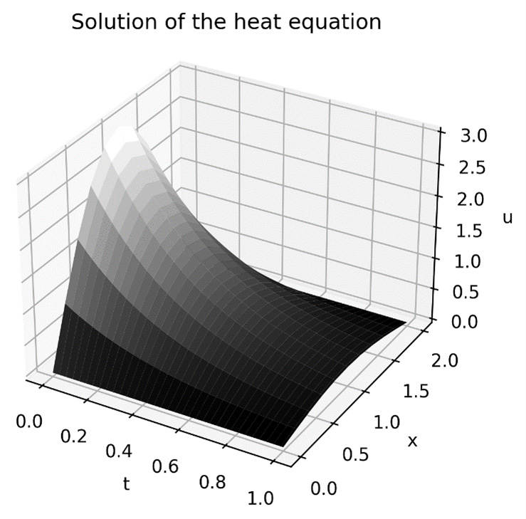
Figure 3.6 -Numerical solution of the heat equation over the range

Along the axis, we can see that the overall shape is similar to the shape of the initial profile but becomes flatter as time progresses. Along the axis, the surface exhibits the exponential decay that is characteristic of cooling systems.

How it works...

The finite difference method works by replacing each of the derivatives with a simple fraction that involves only the value of the function, which we can estimate. To implement this method, we first break down the spatial range and time range into a number of discrete intervals, separated by mesh points. This process is called discretization. Then, we use the differential equation and the initial conditions and boundary conditions to form successive approximations, in a manner very similar to the time-stepping methods used by the solve_ivp routine in the Solving simple differential equations numerically recipe.

In order to solve a partial differential equation such as the heat equation, we need at least three pieces of information. Usually, for the heat equation, this will come in the form of boundary conditions for the spatial dimension, which tell us what the behavior is at either end of the rod, and initial conditions for the time dimension, which is the initial temperature profile over the rod.

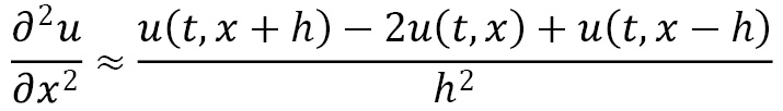
The finite difference scheme described previously is usually referred to as the forward time cen (FTCS) scheme, since we use the forward finite difference to estimate the time derivative and the central finite difference to estimate the (second-order) spatial derivative. The formula for the first-order finite difference approximation is shown here:

Similarly, the second-order approximation is given by the following formula:

Substituting these approximations into the heat equation, and using the approximation for the value of after time steps at the spatial point, we get this:

This can be rearranged to obtain the following formula:

Roughly speaking, this equation says that the next temperature at a given point depends on the surrounding temperatures at the previous time. This also shows why the condition on the r value is necessary; if the condition does not hold, the middle term on the right-hand side will be negative.

We can write this system of equations in matrix form:

Here, is a vector containing the approximation and matrix , which was defined in step 4. This matrix is tridiagonal, which means the nonzero entries appear on, or adjacent to, the leading diagonal. We use the diag routine from the SciPy sparse module, which is a utility for defining these kinds of matrices. This is very similar to the process described in the Solving equations recipe of this chapter. The first and last rows of this matrix have zeros, except in the top left and bottom right, respectively, that represent the (non-changing) boundary conditions. The other rows have coefficients that are given by the finite difference approximations for the derivatives on either side of the differential equation. We first create diagonal entries and entries above and below the diagonal, and then we use the diags routine to create a sparse matrix. The matrix should have rows and columns, to match the number of mesh points, and we set the data type as double-precision floats and compressed sparse row (CSR) format.

The initial profile gives us the vector , and from this first point, we can compute each subsequent time step by simply performing a matrix multiplication, as we saw in step 7.

There’s more...

The method we describe here is rather crude since the approximation can become unstable, as we mentioned, if the relative sizes of time steps and spatial steps are not carefully controlled. This method is explicit since each time step is computed explicitly using only information from the previous time step. There are also implicit methods, which give a system of equations that can be solved to obtain the next time step. Different schemes have different characteristics in terms of the stability of the solution.

When the function is not 0, we can easily accommodate this change by using the following assignment:

Here, the function is suitably vectorized to make this formula valid. In terms of the code used to solve the problem, we need only include the definition of the function and then change the loop of the solution, as follows:

for i in range(steps):
       u[i+1, :] = A @ u[i, :] + f(t[i], x)

Physically, this function represents an external heat source (or sink) at each point along the rod. This may change over time, which is why, in general, the function should have both and as arguments (though they need not both be used).

The boundary conditions we gave in this example represent the ends of the rod being kept at a constant temperature of 0. These kinds of boundary conditions are sometimes called Dirichlet boundary conditions. There are also Neumann boundary conditions, where the derivative of the function is given at the boundary. For example, we might have been given the following boundary conditions:

This could be interpreted physically as the ends of the rod being insulated so that heat cannot escape through the endpoints. For such boundary conditions, we need to modify the matrix slightly, but otherwise, the method remains the same. Indeed, inserting an imaginary value to the left of the boundary and using the backward finite difference at the left-hand boundary (), we obtain the following:

Using this in the second-order finite difference approximation, we get this:

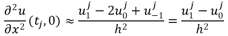
This means that the first row of our matrix should contain , then , followed by . Using a similar computation for the right-hand limit gives a similar final row of the matrix:

diag = [1-r, *(1-2*r for _ in range(N-1)), 1-r]
abv_diag = [*(r for _ in range(N))]
blw_diag = [*(r for _ in range(N))]
A = sparse.diags([blw_diag, diag, abv_diag], (-1, 0, 1),
                 shape=(N+1, N+1), dtype=np.float64,
                 format="csr")

For more complex problems involving partial differential equations, it is probably more appropriate to use a finite elements solver. Finite element methods use a more sophisticated approach for computing solutions than partial differential equations, which are generally more flexible than the finite difference method we saw in this recipe. However, this comes at the cost of requiring more setup that relies on more advanced mathematical theory. On the other hand, there is a Python package for solving partial differential equations using finite element methods such as FEniCS (fenicsproject.org). The advantage of using packages such as FEniCS is that they are usually tuned for performance, which is important when solving complex problems with high accuracy.

See also

The FEniCS documentation gives a good introduction to the finite element method and a number of examples of using the package to solve various classic partial differential equations. A more comprehensive introduction to the method and the theory is given in the following book: Johnson, C. (2009). Numerical solution of partial differential equations by the finite element method. Mineola, N.Y.: Dover Publications.

For more details on how to produce three-dimensional surface plots using Matplotlib, see the Surface and contour plots recipe from Chapter 2, Mathematical Plotting with Matplotlib.

Using discrete Fourier transforms for signal processing

One of the most useful tools coming from calculus is the Fourier transform (FT). Roughly speaking, the FT changes the representation, in a reversible way, of certain functions. This change of representation is particularly useful in dealing with signals represented as a function of time. In this instance, the FT takes the signal and represents it as a function of frequency; we might describe this as transforming from signal space to frequency space. This can be used to identify the frequencies present in a signal for identification and other processing. In practice, we will usually have a discrete sample of a signal, so we have to use the discrete Fourier transform (DFT) to perform this kind of analysis. Fortunately, there is a computationally efficient algorithm, called the FFT, for applying the DFT to a sample.

We will follow a common process for filtering a noisy signal using the FFT. The first step is to apply the FFT and use the data to compute the power spectral density (PSD) of the signal. Then, we identify peaks and filter out the frequencies that do not contribute a sufficiently large amount to the signal. Then, we apply the inverse FFT to obtain the filtered signal.

In this recipe, we use the FFT to analyze a sample of a signal and identify the frequencies present and clean the noise from the signal.

Getting ready

For this recipe, we will only need the NumPy and Matplotlib packages imported as np and plt, as usual. We will need an instance of the default random number generator, created as follows:

rng = np.random.default_rng(12345)

Now, let’s see how to use the DFT.

How to do it...

Follow these instructions to use the FFT to process a noisy signal:

1. We define a function that will generate our underlying signal:

   def signal(t, freq_1=4.0, freq_2=7.0):

       return np.sin(freq_1 * 2 * np.pi * t) + np.sin(

           freq_2 * 2 * np.pi * t)
2. Next, we create our sample signal by adding some Gaussian noise to the underlying signal. We also create an array that holds the true signal at the sample values for convenience later:

   sample_size = 2**7 # 128

   sample_t = np.linspace(0, 4, sample_size)

   sample_y = signal(sample_t) + rng.standard_normal(

       sample_size)

   sample_d = 4./(sample_size - 1) # Spacing for linspace array

   true_signal = signal(sample_t)
3. We use the fft module from NumPy to compute DFTs. We import this from NumPy before we start our analysis:

   from numpy import fft
4. To see what the noisy signal looks like, we can plot the sample signal points with the true signal superimposed:

   fig1, ax1 = plt.subplots()

   fig1, ax1 = plt.subplots()

   ax1.plot(sample_t, sample_y, "k.",

            label="Noisy signal")

   ax1.plot(sample_t, true_signal, "k--",

            label="True signal")

   ax1.set_title("Sample signal with noise")

   ax1.set_xlabel("Time")

   ax1.set_ylabel("Amplitude")

   ax1.legend()

The plot created here is shown in Figure 3.7. As we can see, the noisy signal does not bear much resemblance to the true signal (shown with the dashed line):

Figure 3.7 – Noisy signal sample with true signal superimposed

5. Now, we will use the DFT to extract the frequencies that are present in the sample signal. The fft routine in the fft module performs the DFT:

   spectrum = fft.fft(sample_y)
6. The fft module provides a routine for constructing the appropriate frequency values called fftfreq. For convenience, we also generate an array containing the integers at which the positive frequencies occur:

   freq = fft.fftfreq(sample_size, sample_d)

   pos_freq_i = np.arange(1, sample_size//2, dtype=int)
7. Next, compute the PSD of the signal, as follows:

   psd = np.abs(spectrum[pos_freq_i])**2 + np.abs(

       spectrum[-pos_freq_i])**2
8. Now, we can plot the PSD of the signal for the positive frequencies and use this plot to identify frequencies:

   fig2, ax2 = plt.subplots()

   ax2.plot(freq[pos_freq_i], psd, "k")

   ax2.set_title("PSD of the noisy signal")

   ax2.set_xlabel("Frequency")

   ax2.set_ylabel("Density")

The result can be seen in Figure 3.8. We can see in this diagram that there are spikes at roughly 4 and 7, which are the frequencies of the signal that we defined earlier:

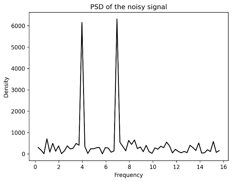
Figure 3.8 – PSD of a signal generated using the FFT

9. We can identify these two frequencies to try to reconstruct the true signal from the noisy sample. All of the minor peaks that appear are not larger than 2,000, so we can use this as a cut-off value for the filter. Let’s now extract from the list of all positive frequency indices the (hopefully 2) indices that correspond to the peaks above 2,000 in the PSD:

   filtered = pos_freq_i[psd > 2e3]
10. Next, we create a new, clean spectrum that contains only the frequencies that we have extracted from the noisy signal. We do this by creating an array that contains only 0, and then copying the value of spectrum from those indices that correspond to the filtered frequencies and the negatives thereof:

    new_spec = np.zeros_like(spectrum)

    new_spec[filtered] = spectrum[filtered]

    new_spec[-filtered] = spectrum[-filtered]
11. Now, we use the inverse FFT (using the ifft routine) to transform this clean spectrum back to the time domain of the original sample. We take the real part using the real routine from NumPy to eliminate the erroneous imaginary parts:

    new_sample = np.real(fft.ifft(new_spec))
12. Finally, we plot this filtered signal over the true signal and compare the results:

    fig3, ax3 = plt.subplots()

    ax3.plot(sample_t, true_signal, color="#8c8c8c",

             linewidth=1.5, label="True signal")

    ax3.plot(sample_t, new_sample, "k--",

             label="Filtered signal")

    ax3.legend()

    ax3.set_title("Plot comparing filtered signal and true signal")

    ax3.set_xlabel("Time")

    ax3.set_ylabel("Amplitude")

The result of step 11 is shown in Figure 3.9. We can see that the filtered signal closely matches the true signal, except for some small discrepancies:

Figure 3.9 – Filtered signal generated using FFTs superimposed over the true signal

We can see in Figure 3.9 that the filtered signal (dashed line) fits fairly closely over the true signal (lighter solid line). It captures most (but not all) of the oscillations of the true signal.

How it works...

The FT of a function is given by the following integral:

The DFT is given by the following integral:

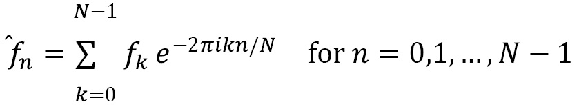
Here, the values are the sample values as complex numbers. The DFT can be computed using the preceding formula, but in practice, this is not efficient. Computing using this formula is . The FFT algorithm improves the complexity to , which is significantly better. The book Numerical Recipes (full bibliographic details given in the Further reading section) gives a very good description of the FFT algorithm and the DFT.

We will apply the DFT to a sample generated from a known signal (with known frequency modes) so that we can see the connection between the results we obtain and the original signal. To keep this signal simple, we created a signal that has only two frequency components with values 4 and 7. From this signal, we generated a sample that we analyzed. Because of the way the FFT works, it is best if the sample has a size that is a power of 2; if this isn’t the case, we can pad the sample with zero elements to make this the case. We add some Gaussian noise to the sample signal, which takes the form of a normally distributed random number.

The array returned by the fft routine contains elements, where is the sample size. The element that index 0 corresponds to is the 0 frequency or DC shift. The next elements are the values corresponding to the positive frequencies, and the final elements are the values corresponding to the negative frequencies. The actual values of the frequencies are determined by the number of sampled points and the sample spacing, which, in this example, is stored in sample_d.

The PSD at the frequency is given by the following formula:

Here, represents the FT of the signal at frequency . The PSD measures the contribution of each frequency to the overall signal, which is why we see peaks at approximately 4 and 7. Since Python indexing allows us to use negative indices for elements starting from the end of the sequence, we can use the positive index array to get both the positive and negative frequency elements from spectrum.

In step 9, we identified the indices of the two frequencies that peak above 2,000 on the plot. The frequencies that correspond to these indices are 3.984375 and 6.97265625, which are not exactly equal to 4 and 7 but are very close. The reason for this discrepancy is the fact that we have sampled a continuous signal using a finite number of points. (Using more points will, of course, yield better approximations.)

In step 11, we took the real part of the data returned from the inverse FFT. This is because, technically speaking, the FFT works with complex data. Since our data contained only real data, we expect that this new signal should also contain only real data. However, there will be some small errors made, meaning that the results are not totally real. We can remedy this by taking the real part of the inverse FFT. This is appropriate because we can see that the imaginary parts are very small.

We can see in Figure 3.9 that the filtered signal very closely matches the true signal, but not exactly. This is because, as mentioned previously, we are approximating a continuous signal with a relatively small sample.

There’s more...

Signal processing in a production setting would probably make use of a specialized package, such as the signal module from scipy, or some lower-level code or hardware to perform filtering or cleaning of a signal. This recipe should be taken as more of a demonstration of the use of FFT as a tool for working with data sampled from some kind of underlying periodic structure (the signal). FFTs are useful for solving partial differential equations, such as the heat equation seen in the Solving partial differential equations numerically recipe.

See also

More information about random numbers and the normal distribution (Gaussian) can be found in Chapter 4, Working with Randomness and Probability.

Automatic differentiation and calculus using JAX

JAX is a linear algebra and automatic differentiation framework developed by Google for ML. It combines the capabilities of Autograd and its Accelerated Linear Algebra (XLA) optimizing compiler for linear algebra and ML. In particular, it allows us to easily construct complex functions, with automatic gradient computation, that can be run on Graphics Processing Units (GPUs) or Tensor Processing Units (TPUs). On top of all of this, it is relatively simple to use. In this recipe, we see how to make use of the JAX just-in-time (JIT) compiler, get the gradient of a function, and make use of different computation devices.

Getting ready

For this recipe, we need the JAX package installed. We will make use of the Matplotlib package, with the pyplot interface imported as plt as usual. Since we’re going to plot a function of two variables, we also need to import the mplot3d module from the mpl_toolkits package.

How to do it…

The following steps show how to define a JIT-compiled function using JAX, compute the gradient of this function, and use a GPU or TPU to perform calculations:

First, we need to import the parts of the JAX library that we will use:

import jax.numpy as jnp
from jax import grad, jit, vmap

Now, we can define our function, with the @jit decorator applied to tell JAX to JIT compile this function where necessary:

@jit
def f(x, y):
    return jnp.exp(-(x**2 +y**2))

Next, we define a grid and plot our function:

t = jnp.linspace(-1.0, 1.0)
x, y = jnp.meshgrid(t, t)
fig = plt.figure()
ax = fig.add_subplot(projection="3d")
ax.plot_surface(x, y, f(x, y), cmap="gray")
ax.set_title("Plot of the function f(x, y)")
ax.set_xlabel("x")
ax.set_ylabel("y")
ax.set_zlabel("z")

The resulting plot is shown in Figure 3.10:

Figure 3.10 – Plot of a function of two variables computed using JAX

Now, we use the grad function (and the jit decorator) to define two new functions that are the partial derivatives with respect to the first and second arguments:

fx = jit(grad(f, 0))  # x partial derivative
fy = jit(grad(f, 1))  # y partial derivative

To quickly check that these functions are working, we print the values of these functions at :

print(fx(1., -1.), fy(1., -1.))
# -0.27067056 0.27067056

To finish off, let’s plot the partial derivative with respect to :

zx = vmap(fx)(x.ravel(), y.ravel()).reshape(x.shape)
figpd = plt.figure()
axpd = figpd.add_subplot(projection="3d")
axpd.plot_surface(x, y, zx, cmap="gray")
axpd.set_title("Partial derivative with respect to x")
axpd.set_xlabel("x")
axpd.set_ylabel("y")
axpd.set_zlabel("z")

The partial derivative plot is shown in Figure 3.11:

Figure 3.11 – Plot of the partial derivative of the function computed using autodiff in JAX

A quick check confirms that this is indeed a plot of the partial derivative with respect to of the function .

How it works…

JAX is an interesting mix of a JIT compiler, with an emphasis on fast linear algebra operations, combined with the power of Autograd, with support for acceleration devices (and several other features that we don’t use here). The JIT compilation works by tracing the linear algebra operations performed on the JAX version of the NumPy library and constructing an intermediate representation of the function in a form that can be understood by the XLA compiler. For any of this to work, you need to make sure that you only use the NumPy module from JAX (jax.numpy) rather than the real NumPy. JAX also provides a version of the SciPy package.

One caveat of this approach is that the functions must be pure: they should not have side effects beyond the return value, and should not depend on any data not passed by arguments. It might still work if this is not the case, but you might get unexpected results—remember that the Python version of the function might only be executed once. Something else to consider is that, unlike NumPy arrays, JAX NumPy arrays cannot be updated in place using index notation and assignment. This, and several other current important caveats, are listed in the JAX documentation (refer to the following section, See also…).

The jit decorator instructs JAX to construct compiled versions of the function where appropriate. It might actually produce several compiled versions depending on the types of arguments provided (for example, a different compiled function for scalar values versus array values).

The grad function takes a function and produces a new function that computes the derivative with respect to the input variable. If the function has more than one input variable, then this is the partial derivative with respect to the first argument. The second optional argument, argnums, is used to specify which derivatives to compute. In the recipe, we have a function of two variables and used the grad(f, 0) and grad(f, 1) commands to get the functions representing the two partial derivatives of the f function.

Most of the functions from jax.numpy have the same interface as from numpy—we see a few of these functions in the recipe. The difference is that JAX versions produce arrays that are stored correctly for the accelerator device if one is used. We can use these arrays in contexts that expect NumPy arrays, such as plotting functions, without any issues.

In step 5 of the recipe, we printed the value of the two partial derivatives. Notice that we used the values 1. and -1.. It is important to note that using the integer equivalent 1 and -1 would have failed because of the way JAX handles floating-point numbers. (Since most GPU devices do not handle double-precision floating-point numbers well, the default float type in JAX is float32.)

In step 6, we computed the derivative over the same region as the function. To do this, we had to flatten the and arrays and then use the vmap function to vectorize the fx derivative before reshaping the result. There is a complication in the way that grad works, which means that fx does not vectorize in the way we expect.

There’s more…

JAX is designed to scale well as needs change, so lots of the components are designed with concurrency in mind. For instance, the random numbers module provides a random number generator that is capable of splitting effectively so that computations can run concurrently without changing the outcome. This wouldn’t be possible, for example, with a Mersenne Twister random generator, which would potentially produce different answers depending on the number of threads used because it doesn’t split in a statistically sound way.

See also

Lots more information can be found in the JAX documentation:

https://jax.readthedocs.io/en/latest/

Solving differential equations using JAX

JAX provides a set of tools for solving a wide array of problems. Solving differential equations—such as initial value problems described in the Solving simple differential equations numerically recipe—should be well within the capabilities of this library. The diffrax package provides various solvers for differential equations leveraging the power and convenience of JAX.

In the earlier recipe, we solved a relatively simple first-order ODE. In this recipe, we’re going to solve a second-order ODE to illustrate the technique. A second-order ODE is a differential equation that involves both the first and second derivatives of a function. To keep things simple, we’re going to solve a linear second-order ODE of the following form:

Here, is a function of to be found. In particular, we’re going to solve the following equation:

The initial conditions are and . (Note that this is a second-order differential equation, so we need two initial conditions.)

Getting ready

Before we can start to solve this equation, we need to do some pen-and-paper work to reduce the second-order equation to a system of first-order differential equations that can be solved numerically. To do this, we make a substitution and . When we do this, we get a system like this:

We also get the initial conditions and .

For this recipe, we will need the diffrax package installed, along with JAX. As usual, we import the Matplotlib pyplot interface under the alias plt. We import jax.numpy under the alias jnp and the diffrax package.

How to do it…

The following steps show how to use JAX and the diffrax library to solve a second-order linear differential equation:

First, we need to set up our function that represents the system of first-order ODEs we constructed in the Getting ready section:

def f(x, y, args):
    u = y[...,0]
    v = y[...,1]
    return jnp.array([v, 3*x**2*v+(1.-x)*u])

Next, we set up the diffrax environment that we will use to solve the equation. We’ll use the solver recommended in the diffrax quickstart guide – see the See also section below for more details. The setup is as follows:

term = diffrax.ODETerm(f)
solver = diffrax.Dopri5()
save_at = diffrax.SaveAt(ts=jnp.linspace(0., 1.))
y0 = jnp.array([0., 1.]) # initial condition

Now, we use the diffeqsolve routine from diffrax to solve the differential equation on the range :

solution = diffrax.diffeqsolve(term, solver, t0=0., t1=2.,
                               dt0=0.1, y0=y0, saveat=save_at)

Now we have solved the equation, we need to extract the values for from the solution object:

x = solution.ts
y = solution.ys[:, 0]  # first column is y = u

Finally, we plot the results on a new figure:

fig, ax = plt.subplots()
ax.plot(x, y, "k")
ax.set_title("Plot of the solution to the second order ODE")
ax.set_xlabel("x")
ax.set_ylabel("y")

The resulting plot is shown in Figure 3.12:

Figure 3.12 – Numerical solution to a second-order linear ODE

We can see that when is close to , the solution is approximately linear, but later on, the solution becomes non-linear. (The range might be too small to see the interesting behavior of this system.)

How it works…

diffrax is built on top of JAX and provides various solvers for differential equations. In the recipe, we used the Dormand-Prince 5(4) Dopri5 solver class, which is another example of a Runge-Kutta method for solving ODEs similar to the Runge-Kutta-Fehlberg method we saw in an earlier recipe.

Behind the scenes, diffrax translates the ODE initial value problem into a controlled differential equation (CDE), which it then solves. This makes diffrax able to solve other kinds of differential equations besides these simple ODEs shown here; one of the goals of the library is to provide tools for numerically solving stochastic differential equations (SDEs). Since it is based on JAX, it should be easy to integrate this into other JAX workflows. It also has support for backpropagation through various adjoint methods.

See also

More information about the diffrax library and the methods it contains can be found in the documentation:

https://docs.kidger.site/diffrax

Further reading

Calculus is a very important part of every undergraduate mathematics course. There are a number of excellent textbooks on calculus, including the classic textbook by Spivak and the more comprehensive course by Adams and Essex:

• Spivak, M. (2006). Calculus. 3rd ed. Cambridge: Cambridge University Press.
• Adams, R. and Essex, C. (2018). Calculus: A Complete Course. 9th ed. Don Mills, Ont: Pearson.

A good source for numerical differentiation and integration is the classic Numerical Recipes book, which gives a comprehensive description of how to solve many computational problems in C++, including a summary of the theory:

• Press, W., Teukolsky, S., Vetterling, W. and Flannery, B. (2007). Numerical Recipes: The Art of Scientific Computing. 3rd ed. Cambridge: Cambridge University Press.