CHAPTER 3
Machine Learning
“Before we work on artificial intelligence why don't we do something about natural stupidity?”
—Steve Polyak (American Neurologist)
CHAPTER OUTLINE
3.1 Introduction
As you saw in Chapter 1, AI covers a broad area, and one of most important aspects of AI is machine learning.
Machine learning (ML) is basically a set of mathematical algorithms developed in the 1980s. Machine learning is an important subset of AI, and it is the science that aims to teach computers, or machines, to learn from data and to analyze data automatically, without human intervention. It includes a set of mathematical algorithms that can make a decision or, more accurately, predict the results for a given set of data. The term machine learning was coined by Arthur Samuel, an American pioneer in computer science and artificial intelligence, in 1959 when he was working at IBM. In 1997, a more modern definition of machine learning was provided by Tom Mitchell as “A computer program is said to learn from experience E with respect to some class of tasks T and performance measure P, if its performance at tasks in T, as measured by P, improves with experience E.”
Machine learning can be divided into these four different categories:
- Supervised learning: In supervised learning, models are trained with labeled data. During the training, algorithms continuously adjust the parameters of models until the error calculated between the output and the desired output for a given input is minimized. Supervised learning is typically used in classification and regression. Classification means to identify, for a given input sample, which class (or category) something belongs to, such as dog or cat, male or female, cancer or no cancer, genuine or fake, and so on. The most popular supervised learning algorithms are the following: support vector machines, naive Bayes, linear discriminant analysis, decision trees, k-nearest neighbor algorithm, neural networks (multilayer perceptron), and similarity learning. Regression means, for the given data, fit the data with a model to get the best-fit parameters. The most popular regression algorithms are linear regression, logistic regression, and polynomial regression.
- Unsupervised learning: In unsupervised learning, models are fed with unlabeled data. The algorithms will study the data and divide it into groups according to features. Unsupervised learning is typically used for clustering and association. Clustering means dividing the data into groups. The most popular clustering algorithm is K-means clustering. Association means to discover rules that describe the majority portion of the data. A popular association algorithm is the Apriori algorithm.
- Semi-supervised learning: In semi-supervised learning, both labeled data and unlabeled data are used. This is particularly useful when not all the data can be labeled. The basic procedure is to group the data into different clusters using an unsupervised learning algorithm and then using the existing labeled data to label the rest of the unlabeled data. The most popular semi-supervised learning algorithms include self-training, generative methods, mixture models, and graph-based methods. Semi-supervised learning can typically be used in speech analysis, internet content classification, and protein sequence classification.
- Reinforcement learning: In reinforcement learning, algorithms learn to find, through trial and error, which actions can yield the maximum cumulative reward. Reinforcement learning is widely used in robotics, video gaming, and navigation.
Today, machine learning has been used in a variety of applications. In healthcare, for example, machine learning has been used for early disease detection, cancer diagnosis, and drug discovery. In social media, machine learning has been used for sentiment analysis, for example, to decide whether a comment is positive or negative. In banking, machine learning has been used for fraud detection. In e-commerce, machine learning has been used for recommending songs, movies, or products based on customers' previous shopping records.
3.2 Supervised Learning: Classifications
Supervised learning is the most important part of machine learning. Supervised learning can be used for classification and regression. We will introduce classification in this section and regression in the next section based on the popular Scikit-Learn library (https://scikit-learn.org/).
Classification means for a given sample you need to predict which category it belongs to. The best-known classification example in the field of machine learning is iris flower classification, which is to classify iris flowers among three species (Setosa, Versicolor, or Virginica) based on the measured length and width of the sepals and petals. Another popular classification is breast cancer classification. In this example, a set of measurement results (such as radius, area, perimeter, texture, smoothness, compactness, concavity, symmetry, and so on) of a tissue sample are given to decide whether the tissue is malignant or benign.
In machine learning, the following are commonly used terminologies. The categories of flowers, or types of breast tissue (malignant or benign), are called classes. The length and width of sepals and petals, or breast tissue measures, are called features. Data points are called samples, and variables in the models are called parameters.
- Class: The categories of the data
- Features: The measurements
- Samples: The data points
- Parameters: The variables of the model
The most popular supervised learning algorithms are support vector machines, naive Bayes, linear discriminant analysis, principal component analysis, decision trees, random forest, k-nearest neighbor, neural networks (multilayer perceptron), and so on.
Find more details about supervised learning algorithms available by using the Scikit-Learn library:
https://scikit-learn.org/stable/supervised_learning.html
Scikit-Learn Datasets
Datasets are important in machine learning. To make them easy to access, several datasets are provided with the Scikit-Learn library.
Toy Datasets
- Boston house prices dataset
- Iris plants dataset
- Diabetes dataset
- Optical recognition of handwritten digits dataset
- Linnerrud dataset
- Wine recognition dataset
- Breast cancer Wisconsin (diagnostic) dataset
Real-World Datasets
- The Olivetti faces dataset
- The 20 newsgroups text dataset
- The Labeled Faces in the Wild face recognition dataset
- Forest covertypes
- RCV1 dataset
- Kddcup 99 dataset
- California Housing dataset
There are also generated datasets; for more details, see the following:
Support Vector Machines
Support vector machine (SVM) is the best-known supervised learning algorithm. You always start machine learning with SVM. The SVM algorithm can be used for both classification and regression problems. It was developed at AT&T Bell Laboratories by Vladimir Naumovich Vapnik and his colleagues in the 1990s. It is one of the most robust prediction methods, based on the statistical learning framework.
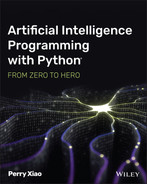
Figure 3.1 shows a simple example of two category classification problems using SVM. You can imagine the two sets of data are two types of flowers, and horizontal and vertical axes are the values of the petals' length and width. SVM will train on this data and create a hyperplane to separate the two sets of the data. In this case, a hyperplane is a straight line. SVM adjusts the position of the hyperplane to maximize the margins to both sets of data. The data points on the margin are called the support vectors. This is a simple two-dimensional, linear classification problem. SVM can also work on three-dimensional, nonlinear classification problems, in which cases a hyperplane could be a plain or more complex curved surface.
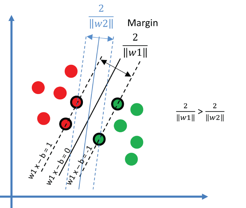
Figure 3.1: The support vector machine with two sets of data points, the hyperplane (solid line), the margin (between two dashed lines), and the support vectors (circled points on the dashed line)
The following is an interesting SVM tutorial that explains how SVM works and how to use SVM with Scikit-Learn:
https://www.datacamp.com/community/tutorials/svm-classification-scikit-learn-python
Now let's look at some Python SVM classification examples. In this chapter, we will use the Scikit-Learn library for classification. You can install the library by typing pip install scikit-learn at the command line, as shown in Chapter 2.
Example 3.1 shows a simple SVM gender classification example based on height, weight, and shoe size. It first uses from sklearn import svm to import the SVM library. It uses an array called X to store four sets of values of height in centimeters, weight in kilos, and shoe size in UK size, and uses an array named y to store four sets of known genders, 0 for Male, 1 for Female. It then trains the SVM classifier and makes a prediction for a given height, weight, and shoe size [[160, 60, 7]].
When you run the code, you will get the following output; [1] here means it is a female:
The Iris dataset is probably the most widely used example for classification problems. Figure 3.2 shows photos of three different types of Iris flowers, Versicolor, Setosa, and Virginica, as well as the location of the sepal and petal.
Iris Versicolor and location of Sepal and Petal
Iris Setosa
(Source: https://upload.wikimedia.org/wikipedia/commons/7/70/Iris_setosa_var._setosa_%282594194341%29.jpg)
Iris Virginica
(Source: https://en.wikipedia.org/wiki/Iris_virginica#/media/File:Iris_virginica_2.jpg)
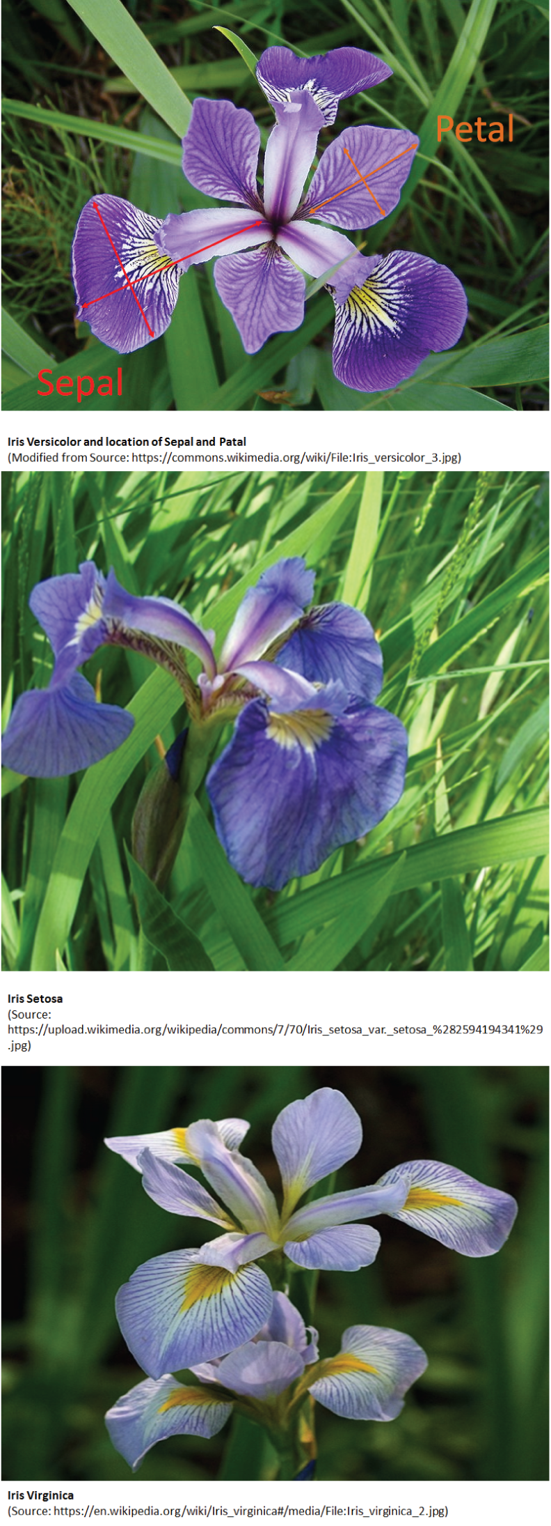
Figure 3.2: Example of three different types of Iris flowers, Versicolor (top), Setosa (middle), and Virginica (bottom), as well as the location of the sepal and petal
(Modified from Source: https://commons.wikimedia.org/wiki/File:Iris_versicolor_3.jpg)
For more details, see the following interesting article about Iris flowers and machine learning:
Example 3.2 shows an SVM classification example for using the Iris dataset that comes with Scikit-Learn. It uses datasets.load_iris() to load the Iris dataset.
In machine learning, data is usually saved in CSV format. Example 3.3 shows an SVM classification example for using the Iris dataset by reading from a CSV file named iris.csv with the function pd.read_csv().
Many people shared their CSV datasets on the Web, such as GitHub.com. You can use the function pd.read_csv() to read the data from a URL just as you would from a local file.
Example 3.4 shows an example of SVM classification, reading a CSV file in the Iris dataset from a URL. The data read by the pd.read_csv() function is stored in a variable called df, which is in Pandas' dataframe format. There are several useful functions in the dataframe format.
df.shape has information about the size of the data, number of rows, and number of columns.
df.head(10) shows the first five rows of the data. By default, df.head() shows the first five rows of the data.
df.tail(10) shows the last five rows of the data. By default, df.tail() shows the last five rows of the data.
df.describe shows the summary of the data.
df.isna() or df.isnull() is a function that shows Not A Number (NAN) or missing numbers. df.isna().sum() shows the number of NANs or missing numbers in each column. df.isna().sum().sum() shows the total number of NANs or missing numbers of the data.
df.dropna() removes the NANs.
df. groupby('species').size() shows the number of each species.
df.hist() plots the histogram of the data.
scatter_matrix() plots the scatter matrix of the data.
pyplot.show() shows the plot.
The following is the output of the previous program. This shows the shape of the data, 150 rows and 5 columns.
This shows the first 10 rows of the data:
This shows the last 10 rows of the data:
This shows the description of the data:
This shows the number of rows with NAN values:
This shows the number of rows for different species:
This shows the prediction result (setosa) for the given input ([[5.4, 3.2]]):
Figure 3.3 shows the histogram plot (top) and matrix scatter plot (bottom) of the previous program. In the histogram, the y-axis shows the number of samples, and the x-axis shows the values of sepal length, sepal width, petal length, and petal width. The matrix scatter plot shows a matrix of 2D scatter plots of the data points with the four features (sepal length, sepal width, petal length, and petal width) against each other. This is useful as it gives an overview of all the data points in terms of all the features so that you can easily see which two features can separate the data better. For example, the scatter plot of petal length against sepal width gives the largest separation of the points into two groups, and in the scatter plot of petal width against sepal length, one group of data was close together in the corner.
On the diagonal of the matrix, as it is the same feature against the same feature, the histogram of the feature is displayed instead.
Figure 3.3: The histogram plot (top) and the matrix plot (bottom) of the Example 3.4
The breast cancer dataset is another popular dataset for classification problems. Example 3.5 shows how to load the breast cancer data from the Scikit-Learn library using the load_breast_cancer() function and then print the feature names, the data, and the target names on-screen.
The following is the output of feature names of the breast cancer dataset. Each feature here is a type of measurement, such as radius, size, texture, smoothness, and so on.
The following is the output of the data, which are the values of each feature of the breast cancer dataset:
The following is the output of the target names of the breast cancer dataset. There are two classes: 0 is malignant, and 1 is benign.
Example 3.6 shows an example of SVM classification for breast cancer. It first loads the breast cancer data's load_breast_cancer() function and then puts the data into a dataframe format, uses features data as X and target as y, and uses train_test_split() to split X and y into training and testing sets. Specifically, 80 percent of data is for training, and 20 percent is for testing. It uses the training data X_train and y_train to train an SVM and uses testing data X_test to make predictions. Finally, it prints the confusion matrix and classification report.
The following is the output of confusion matrix. A confusion matrix is a simple way to show the performance of classification. The results show that there are 66 cancer tissues that have been correctly predicted as cancer, or malignant, and 40 healthy tissues have been correctly predicted as healthy, or benign. There are eight healthy tissues wrongly predicted as cancer, and zero cancer tissue wrongly predicted as healthy.
The following is the output of the classification report, from which you can see the SVM classification has an accuracy of 93 percent:
Naive Bayes
Naive Bayes is another popular supervised learning algorithm, which applies Bayes' theorem with the naive assumption of the probabilities of features for a given dataset. Naive assumption means every feature is independent of the others.
According to Bayes' theorem, the probability of a class (C) happening for a given set of features (X) can be calculated as follows:
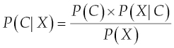
or:
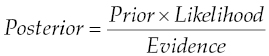
where:
| P(C|X) | is the posterior, the probability of class (C) given features (X). |
| P(C) | is the prior, the probability of class (C). |
| P(X|C) | is the likelihood, the probability of features (X) for given class (C). |
| P(X) | is the prior, probability of features (X). |
To train a naive Bayes classifier, you just need to calculate all the probabilities P(C) of all the classes (types of flowers) for the given features (sepals and petals' length and width) and evidence P(X). For a given dataset, P(C) and P(X) are constants. Hence, they are saved for future use. Given a sample X, the likelihood P(X|C) will be calculated, and the posterior P(C|X) can be calculated.
For more details, see the following resources:
https://scikit-learn.org/stable/modules/naive_bayes.html
https://en.wikipedia.org/wiki/Naive_Bayes_classifier
Example 3.7 shows an example of a naive Bayes classification for irises. In this case, it uses X, y = load_iris(return_X_y=True) to load the iris data and returns the data as X and y, where X includes all four features of that data. It then trains the naive Bayes classifier model and makes a prediction for a given sample with the sepal's length and width and the petal's length and width.
For a large amount of data, you can save the trained model to a file and load the model from the file later. Saving the model to a file is called serialization.
You can use Sklearn's joblib for this.
from sklearn.externals import joblibjoblib.dump(clf, 'model.pkl')
Once the model has been saved, you can then load this model into memory with a single line of code. Loading the model back into your workspace is called deserialization.
clf2 = joblib.load('model.pkl')
Linear Discriminant Analysis
Linear discriminant analysis (LDA) is one of the most commonly used dimension reduction techniques in machine learning. The goal is to project a dataset onto a lower-dimensional space to separate them better into different classes and to reduce computational costs.
Figure 3.4 illustrates how LDA works. For a given set of data with three classes, measured on two features (x1 and x2), all mingled together, it is difficult to separate them; see Figure 3.4 (left). LDA will try to find new axes, see the dashed lines, and project the data to the new axes (LDA1 and LDA2); it will adjust the axes according to the means and variances of each group of data to best separate the data into different classes. After LDA, you can plot the data according to new axes (LDA1 and LDA2), which can improve the separation, as shown in Figure 3.4 (right).
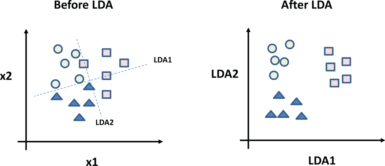
Figure 3.4: LDA: a set of given data before LDA (left) and the data after LDA (right)
LDA basically projects the data from one dimension linearly into another dimension. Apart from LDA, there is also nonlinear discriminant analysis.
- Quadratic discriminant analysis (QDA)
- Flexible discriminant analysis (FDA)
- Regularized discriminant analysis (RDA)
For more details about LDA and QDA in the Scikit-Learn library, see the following:
https://scikit-learn.org/stable/modules/lda_qda.html
Here is an interesting YouTube video from StatQuest by Josh Starmer that clearly explains LDA:
https://www.youtube.com/watch?v=azXCzI57Yfc
Example 3.8 shows a simple LDA classification example. In this example, it uses make_classification() to generate a simulated dataset as X and y, with 1,000 samples and 4 features. It then trains the LDA classifier model and makes a prediction for a given sample with four values.
Principal Component Analysis
Principal component analysis (PCA) is another common dimension reduction technique in machine learning, similar to LDA. The goal is also to project a dataset onto a lower-dimensional space. LDA aims to create new axes (called discriminants) to maximize class separation, while PCA aims to find new axes (called components) to maximize variance (the average of the squared differences from the mean). In PCA, the number of the principal components is less than or equal to the number of original variables, the first principal component will have the largest possible variance, and each succeeding component in turn has the largest variance possible under the constraint that it is orthogonal to the preceding components. Figure 3.5 illustrates the original data plotted according to its features (x1 and x2) and the data after PCA, plotted according to new axes (PCA1 and PCA2).
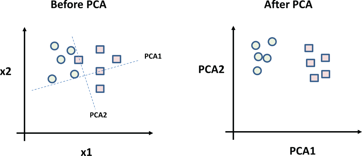
Figure 3.5: PCA: a set of given data before PCA (left) and the data after PCA (right)
Figure 3.6 shows an interesting article about LDA, which also shows a comparison of LDA and PCA. LDA can be described as a supervised algorithm, as it aims to maximize separation of the classes, while PCA can be described as an unsupervised algorithm, as it ignores the classes and aims to maximize the variance of the data. The author also provides a vivid explanation of the Iris dataset and a Python implement of LDA with step-by-step instructions. So, if you are interested in learning the mathematical background of LDA, this is an interesting article to read.
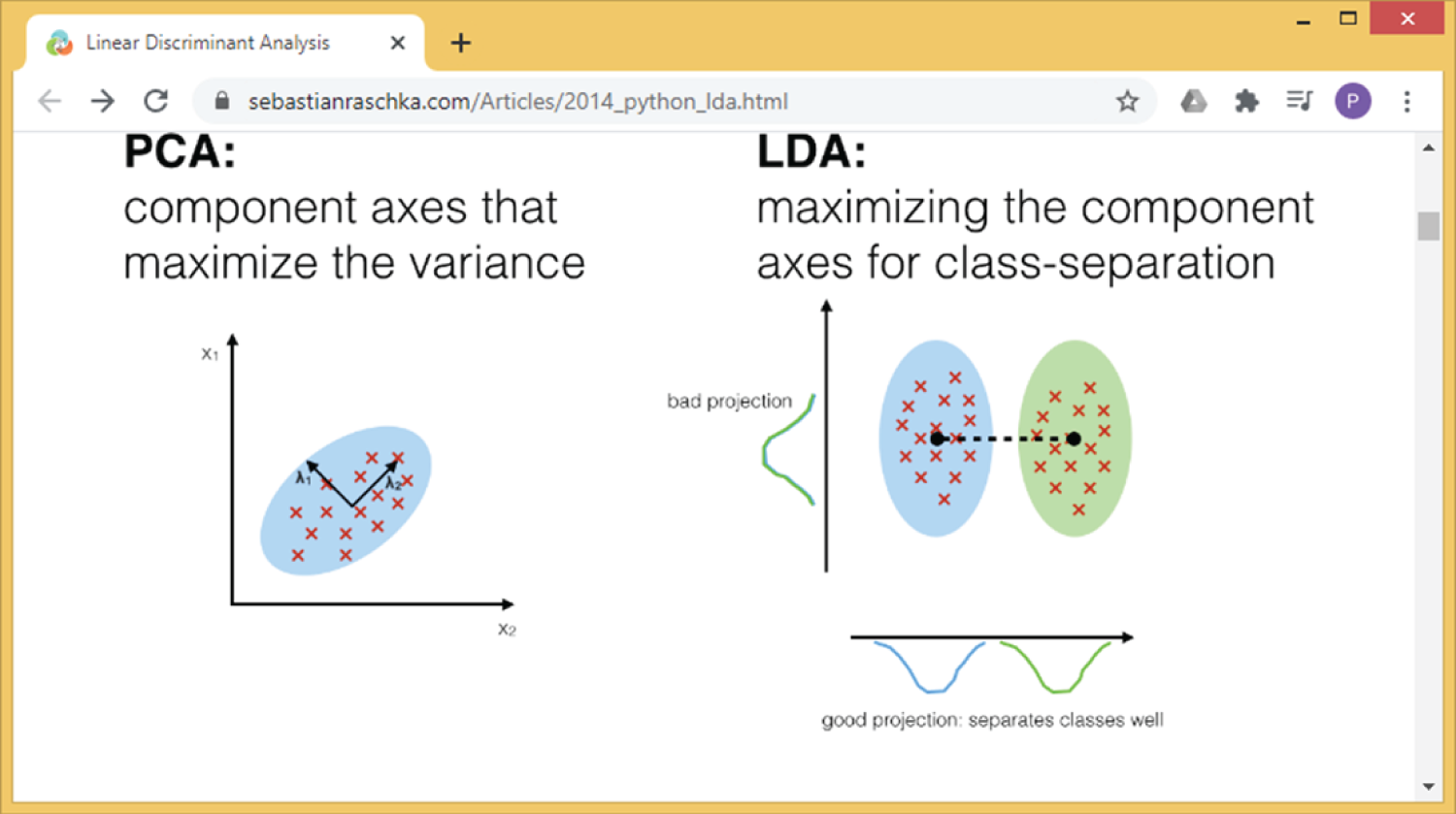
Figure 3.6: An article about linear discriminant analysis, which compares PCA and LDA
(Source: https://sebastianraschka.com/Articles/2014_python_lda.html)
This is another article that shows the step-by-step Python implementation of PCA:
https://sebastianraschka.com/Articles/2014_pca_step_by_step.html
Here is another interesting YouTube video from StatQuest by Josh Starmer that clearly explains PCA:
https://www.youtube.com/watch?app=desktop&v=FgakZw6K1QQ
Example 3.9 shows some simple PCA example code. In this example, it uses make_classification() to generate a simulated dataset as X and y, with 1,000 samples and 4 features. It then trains the PCA model and displays the PCA results. Although PCA cannot be used directly for classification, it is commonly used as a dimension reduction technique before classification.
Example 3.10 shows a simple PCA example for the Iris dataset. In this example, it loads the Iris dataset as X and y arrays, plots the original X data, trains the PCA model, and transforms the X into PCA domains. It finally displays the transformed X in PCA domains using the first two PCA components, PCA1 and PCA2. Figure 3.7 shows the output of Example 3.10, and you can clearly see the differences of original data and PCA-transformed data.
Decision Tree
A decision tree is one of the most widely used, nonparametric, supervised learning methods, and it can be used for both classification and regression problems. A set of rules can be derived from a decision tree (an upside-down tree). Decisions can be made based on the derived rules. In a decision tree, a note is the query variable, and the edge is the value of the query variable. A decision process starts from the tree root and goes down to branches and leaves. Hence, each branch represents an if-then rule. For example, the first branch of the decision tree in Figure 3.8 represents the rule: if the weather forecast is sunny and the humidity is high, then there is no play of golf. The deeper the tree is, the more complex the rules and the model. The goal of a decision tree training algorithm is to create a decision tree based on a dataset and finally produce a set of rules for prediction given a sample.
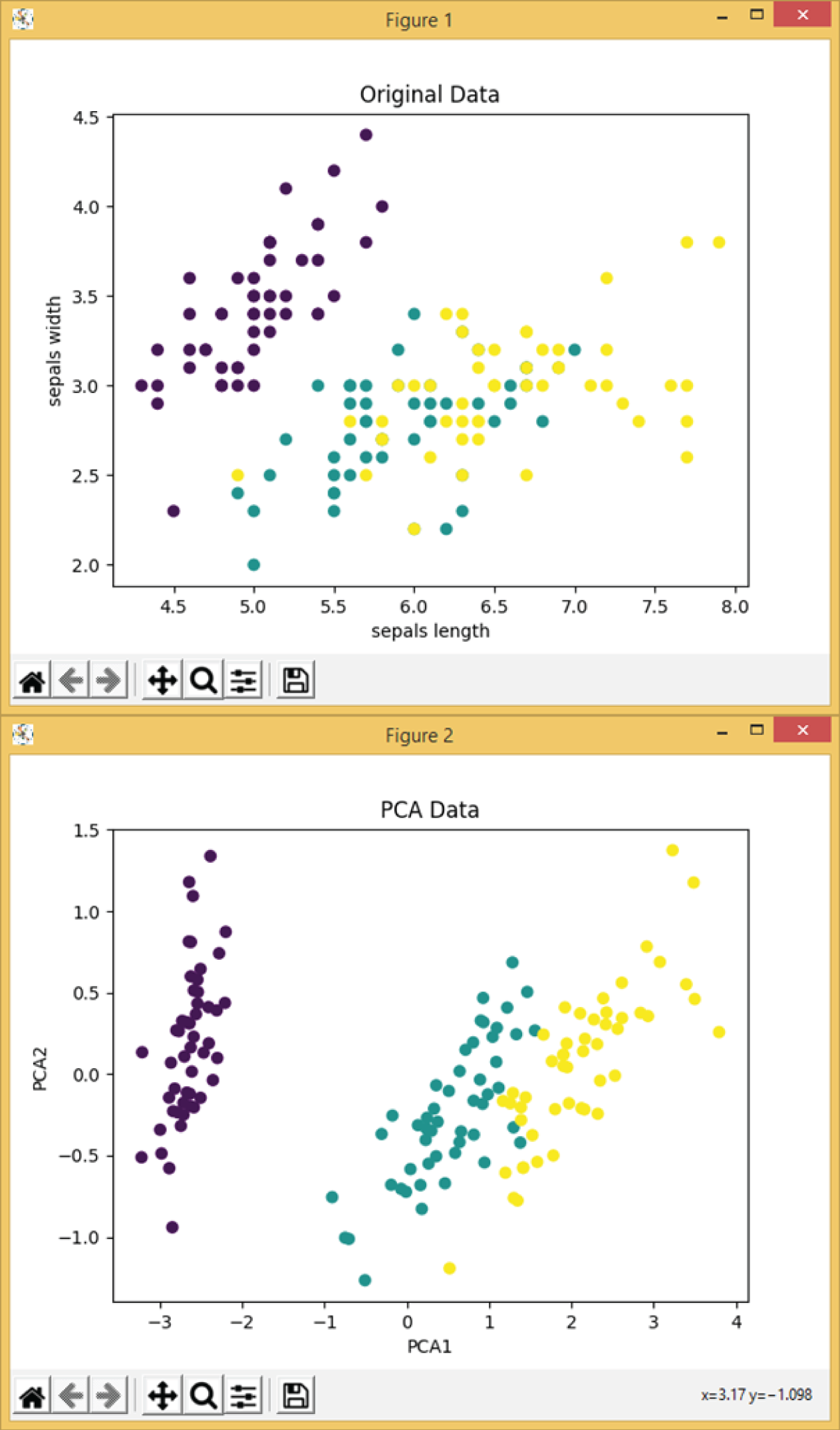
Figure 3.7: The scatter plot of the original Iris dataset (top) and the scatter plot of first two components of the corresponding PCA results (bottom)

Figure 3.8: A simple decision tree to decide whether to play golf
Figure 3.8 shows a simple decision tree to determine whether to play golf.
Here is a similar example of a decision tree:
https://www.geeksforgeeks.org/decision-tree/
For more details of a decision tree in the Scikit-Learn library, see the following page:
https://scikit-learn.org/stable/modules/tree.html
Example 3.11 shows an example of decision tree classification for iris flowers. In this case, it uses X, y = load_iris(return_X_y=True) to load the Iris data and returns the data as X and y, using all four features of the data. It then splits the data into the training set and the testing set. It then trains the decision tree classifier model and makes predictions on the testing set. It also calculates and displays the total number of points, as well as the number of points that are correctly predicted.
Random Forest
A random forest is an algorithm that uses multiple decision trees. A single decision tree might not be enough for some applications. A random forest randomly creates a set of decision trees, with each decision tree working on a random subset of data samples. There are different approaches to create random forests.
A random forest then combines the output of individual decision trees to generate the final output. A random forest is an ensemble learning algorithm that can be used for both classification and regression problems. Figure 3.9 illustrates a random forest algorithm; by using multiple decision trees, it can reduce overfitting and improve the performances.
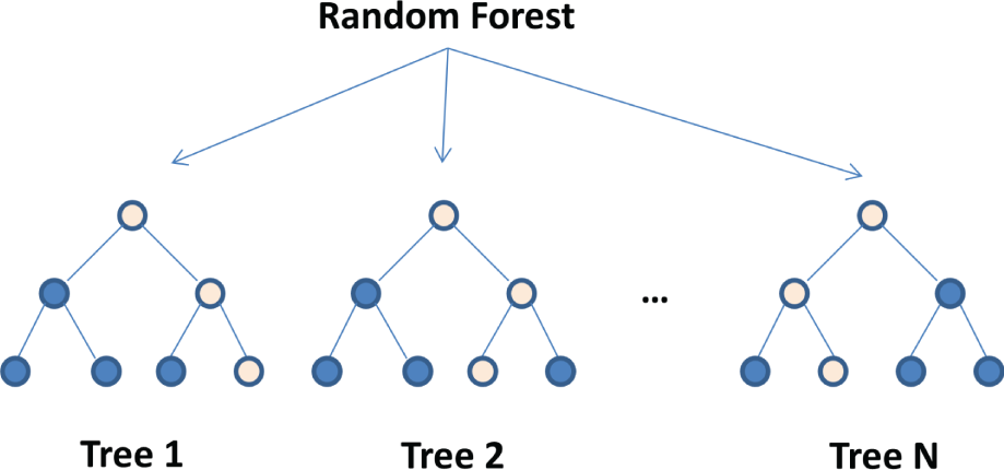
Figure 3.9: Random forest, based on multiple decision trees
Here is an interesting YouTube video from Augmented Startups that explains a random forest in a fun and easy manner:
https://www.youtube.com/watch?v=D_2LkhMJcfY
For more details of a random forest in the Scikit-Learn library, see the following:
https://scikit-learn.org/stable/modules/generated/sklearn.ensemble.RandomForestClassifier.html
Example 3.12 shows an example of a random forest classification for iris flowers. In this case, it uses X, y = load_iris(return_X_y=True) to load the iris data and returns the data as X and y, using all four features of the data. It then trains the random forest classifier model, makes predictions on the test samples, and calculates the number of points predicted correctly.
K-Nearest Neighbors
K-nearest neighbors (K-NN) is a classification (or regression) algorithm that uses K number of nearest points to determine the classification of a dataset. Figure 3.10 shows an example of K-NN classification from Wikipedia. The round point is a test sample, which needs to be classified as either a square or a triangle. Regarding the three nearest neighbors, see the solid circle; it should belong to triangles as there are two triangles and only one square inside the circle. If we choose five nearest neighbors, see the dashed circle; it should belong to the squares, as there are three squares, and two triangles inside the circle. Don't confuse K-nearest neighbors with K-means. K-means is an unsupervised learning algorithm that is mainly used for clustering. We will introduce K-means in section 3.4.
Here is an interesting YouTube video from Simplilearn about K-NN:
https://www.youtube.com/watch?v=4HKqjENq9OU
For more details of K-NN in the Scikit-Learn library, visit this site:
https://scikit-learn.org/stable/modules/neighbors.html
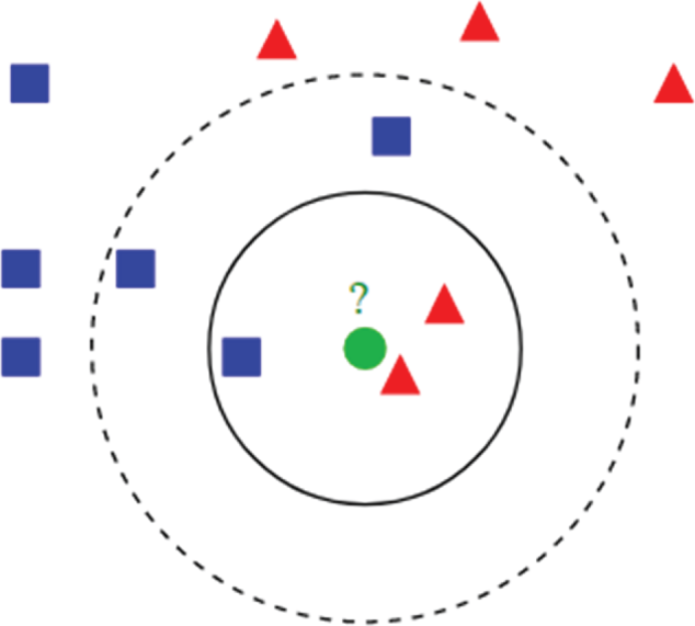
Figure 3.10: Example of K-nearest neighbors
(Source: https://en.wikipedia.org/wiki/K-nearest_neighbors_algorithm#/media/File:KnnClassification.svg)
Example 3.13 shows an example of K-NN classification for iris flowers. In this case, it uses X, y = load_iris(return_X_y=True) to load the iris data and returns the data as X and y arrays, using all four features of that data. It then trains the K-NN classifier model, makes predictions on the test samples, and calculates the number of points predicted correctly.
Neural Networks
A neural network (NN), or artificial neural network (ANN), is a typical three-layer network with one input layer, one hidden layer, and one output layer. Neural networks can be used for both classification and regression. We will have a more detailed description about neural networks in Chapter 4.
For more details of neural networks, also called multilayer perceptron, in the Scikit-Learn library, see the following:
https://scikit-learn.org/stable/modules/neural_networks_supervised.html
Example 3.14 compares different classification models. It uses an array called names to store all the names of the different classifiers and an array called classifiers to store the functions of all the different classifiers. It then loads the iris data and splits it into training and testing sets. A for loop is run through all the classification models, from training the model and making a prediction to calculating the accuracy, as a ratio percentage of the number classified correctly over the total number of points.
The following is the output of the program. It shows that the neural networks gives the best classification results with 98.7 percent of accuracy, compared to other models.
3.3 Supervised Learning: Regressions
Regression is another important aspect of supervised learning. Regression means fitting the data with a mathematical model using a technique called least squares fitting. Regression can be divided into linear regression and nonlinear regression. In linear regression, we fit the data with a straight line (![]() ), where a is the slope, and b is the intercept, as shown in Figure 3.11. For a given dataset, we calculated the sum of the squares of the errors (
), where a is the slope, and b is the intercept, as shown in Figure 3.11. For a given dataset, we calculated the sum of the squares of the errors (![]() ), calculate the distances between the data points and the straight line, and adjust the slope (a) and the intercept (b) of the straight line, until we have reached the smallest sum of the squares (
), calculate the distances between the data points and the straight line, and adjust the slope (a) and the intercept (b) of the straight line, until we have reached the smallest sum of the squares (![]() ), which is why it's called least squares. Linear regression can also be extended to multiple linear regression; in this case, we fit the data with multiple straight lines.
), which is why it's called least squares. Linear regression can also be extended to multiple linear regression; in this case, we fit the data with multiple straight lines.
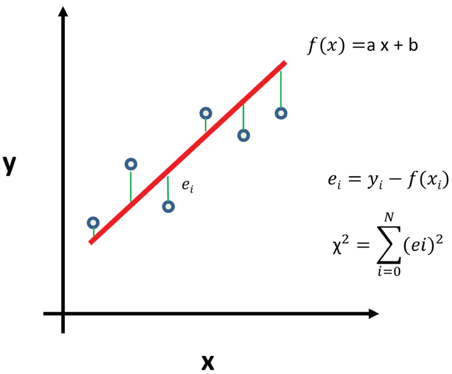
Figure 3.11: Linear regression and the distances between the data points and the straight line
If you are interested in the mathematical details of least squares regression, here is an interesting tutorial about least squares fitting from Wolfram MathWorld:
https://mathworld.wolfram.com/LeastSquaresFitting.html
For nonlinear regression, we fit the data with more complicated mathematical models, such as exponentials and polynomials; see Figure 3.12.
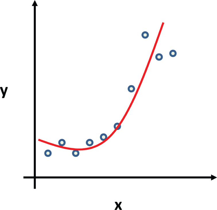
Figure 3.12: Example of nonlinear regression
A common nonlinear regression is logistic regression, where we fit the data with logistic function. Logistic regression is particularly suitable for the data that is dichotomous (binary); see Figure 3.13. It is typically used to predict a binary outcome (pass/fail, win/lose) based on a set of independent variables.
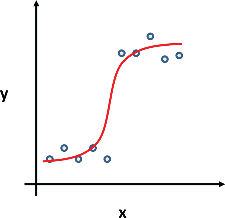
Figure 3.13: Example of logistic regression
Next, let's look at some Python regression examples.
Example 3.15 shows a simple two-dimensional (X and Y) Python linear regression example. It first creates two arrays for x and y values, then performs the linear regression by calling linregress(), and displays the linear regression results: the slope and the intercept. The slope represents the slope of the line, 0.9 is close to 1, which means a line with a 45° slope. The intercept represents the intersection of the line with the y-axis. It also defines a linear function called myfunc() and defines the functions list() and map() to calculate the values of y from the x values of the myfunc()
function. Finally, it uses the functions plt.scatter() and plt.show() to display and plot the original x and y values and the best-fitted line.
The following are the program outputs, the slope, and intercept values. Figure 3.14 shows the plot of the program. The round dots are the x and y values, and the straight line is the best-fit line.
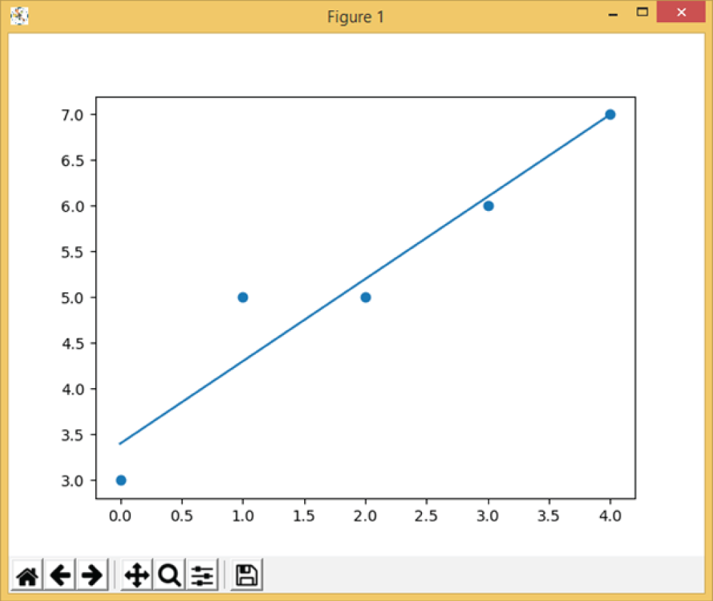
Figure 3.14: The plot of Example 3.15
The Statsmodels library is a powerful statistical model library that comes with a number of mathematical functions, such as regression. To use the library, you will need to install it first, as shown here:
For more details, see this site:
https://www.statsmodels.org/stable/regression.html
Example 3.15a is a similar linear regression example, using the Statsmodels library.
The following is the output of the program:
Figure 3.15 is the plot output of the program.
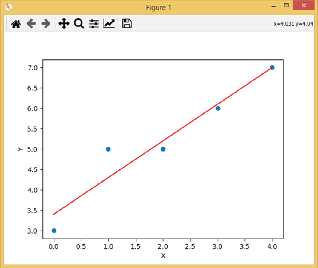
Figure 3.15: The plot of Example 3.15a
Example 3.16 shows a simple example of a two-dimensional (X and Y) Python polynomial regression. It performs the polynomial regression function by calling np.poly1d(np.polyfit(x, y, 3)), where the number 3 means three terms of a polynomial function, which is y = a x3 + b x2 + c x + d.
The following is the program output, the slope, and intercepts values. Figure 3.16 shows the plot of the program; round dots are the x and y values, and the curved line is the best polynomial curve.
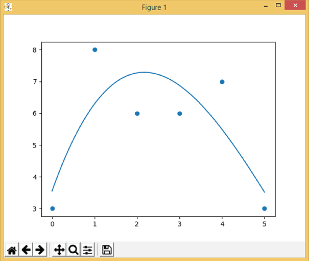
Figure 3.16: The plot of Example 3.16
Example 3.17 shows a simple example of Python least squares fitting. It first creates Numpy arrays for x values and y values. It then defines a function named func() that can be used to fit the x and y values. You can define your own function. Here is a simple exponential decay function: y = a * exp(-b x) +c. It performs the least squares fitting by using the optimization.curve_fit() function and displays the best-fit results.
The following is the output of the program:
Example 3.18 shows a simple example of multiple-dimensional linear regression. It first creates Numpy arrays for x and y values. Please note the format differences of x array and y array. Here, the x array is two-dimensional, while the y array is one-dimensional. It then creates a linear regression model by using the LinearRegression() function and fits the model with the linear relation between the x array and y array. Finally, it displays the linear regression results: the coefficients and the intercept. The coefficient represents the slope of the line. 0.9 is close to 1, which means a line with a slope of 45°. The intercept represents the interception of the line with the y-axis.
The following is the output of the program:
Example 3.19 shows a simple example of Python logistic regression. It first creates Numpy arrays named X and y, which contains a series of X and Y data points. It then performs logistic regression by using the LogisticRegression() function and the fit() function. Finally, it predicts the given sample and displays the result.
The following is the output of the program:
For more details about linear regression, multiple linear regression, nonlinear regression, and logistic regression, visit the Scikit-Learn library:
https://scikit-learn.org/stable/modules/generated/sklearn.linear_model.LinearRegression.html
https://scikit-learn.org/stable/modules/generated/sklearn.linear_model.LogisticRegression.html
3.4 Unsupervised Learning
Unsupervised learning is a type of machine learning technique that does not require you to provide knowledge to supervise the model. The model will discover information on its own. This is different from supervised learning, where you need labeled training data to train the model. Unsupervised learning is useful when you have a large amount of unlabeled data; it can be used for applications such as clustering, association, anomaly detection, etc. Clustering means dividing data points into different groups, called clusters. Association means to establish associations among data points in a large dataset. Anomaly detection means detecting abnormal data points in the dataset. This can be useful for finding fraudulent transactions.
Unsupervised learning includes a number of algorithms for clustering, such as the following:
- Hierarchical clustering
- K-means clustering
- K-NN
- Principal component analysis
- Singular-value decomposition
- Independent component analysis
K-means Clustering
K-means clustering is one of the most commonly used clustering algorithms. It is an iterative algorithm that helps you to find a number of clusters for a given dataset.
The following are the steps of the algorithm, as shown in Figure 3.17:
- Randomly select K points as the center of K clusters, called centroids.
- Calculate the distance between all centroids and the data points. Separate data points into different clusters according to the distances.
- Calculate the mean of all the data of each cluster and move the centroids to the new center of the cluster.
- Repeat steps 2 and 3 for a specified number of iterations until all the clusters are clearly separated.
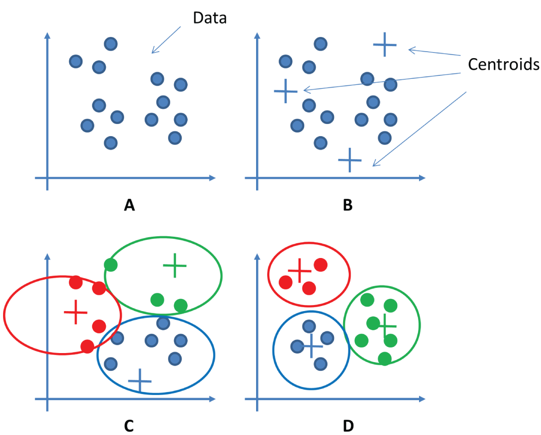
Figure 3.17: The steps of K-means clustering
For more details about K-means clustering, see the following:
https://www.educba.com/k-means-clustering-algorithm/
https://www.edureka.co/blog/k-means-clustering/
Example 3.20 shows a simple example of Python K-means clustering. It first creates a Numpy array named x, which contains two groups of values. It then performs the two-component K-means clustering by using the functions KMeans() and fit(). Finally, it displays the clustering results: the labels of the two clusters and centers of the two clusters and predicts a result for a given sample.
The following is the output of the program:
For more details about K-means clustering, see the Scikit-Learn library:
https://scikit-learn.org/stable/modules/generated/sklearn.cluster.KMeans.html
For more details about unsupervised learning, see the Scikit-Learn library:
3.5 Semi-supervised Learning
Semi-supervised learning lies somewhere between unsupervised learning (without labeled training data) and supervised learning (with labeled training data). Semi-supervised learning is typically used when you have a small amount of labeled data and a large amount of unlabeled data. In semi-supervised learning, data is first divided into different clusters using an unsupervised learning algorithm, and then the existing labeled data is used to label the rest of the unlabeled data.
To make the use of unlabeled data, semi-supervised learning assumes at least one of the following assumptions about the data:
- Continuity assumption: The data points that are closer to each other are more likely to have the same label.
- Cluster assumption: The data can be divided into different clusters, and each cluster shares the same label.
- Manifold assumption: The data lies on a much lower dimension space (called manifold) than the input space. This allows learning to use distances and densities defined on a manifold.
The following are four basic methods that are used in semi-supervised learning:
- Generative models: These are statistical models of the joint probability distribution on a given observable variable and target variable.
- Low-density separation: This attempts to place boundaries in regions with few data points (labeled or unlabeled).
- Graph-based methods: This models the problem space as a graph.
- Heuristic approaches: This uses a practical method to produce solutions that may not be optimal but are sufficient given a limited timeframe.
The following are three practical applications for semi-supervised learning:
- Speech analysis: Such as labeling audio files
- Internet content classification: Such as labeling web pages
- Protein sequence classification: Such as classifying protein families based on their sequence of aminoacids
For more details about semi-supervised learning, visit the following:
https://www.geeksforgeeks.org/ml-semi-supervised-learning/
https://scikit-learn.org/stable/modules/semi_supervised.html
Example 3.21 shows a simple example of Python semi-supervised learning. It first creates a Numpy array named X, which contains two groups of values. It then creates a label variable named labels. All the data points are not labeled, with a value of -1, except the first point labeled as 0, and the last point labeled as 1. This then creates the semi-supervised learning model by calling the LabelSpreading() function, trains the model by calling the label_spread.fit() function, spreads the label by calling the label_spread.transduction_ function, and finally displays the label results.
The following is the program output with the labels before and the labels after the execution of the LabelSpreading() function. As you can see, all the data points have been correctly labeled.
3.6 Reinforcement Learning
Reinforcement learning (RL) is another type of machine learning technique that enables software agents to learn in an interactive environment by trial and error using feedback to maximize accumulative rewards. You have probably already used reinforcement learning in real life; for example, a dog can be taught tricks using reinforcement learning. The dog is the software agent, and the environment is where you teach it tricks. The dog does not understand what you want it to do; it simply tries different actions, and every time when it gets a right action, it gets a reward, or a treat. The next time, the dog learns to do the same thing again and gets the treat again. This is how training a dog works and how reinforcement learning works. Reinforcement learning is currently one of the hottest research topics.
Figure 3.18 shows a schematic diagram of reinforcement learning. In this case, an agent takes actions in an environment. The interpreter interprets these actions into a reward and a state, which are fed back into the agent. The agent adjusts its actions accordingly. This process is repeated many times to maximize the reward.
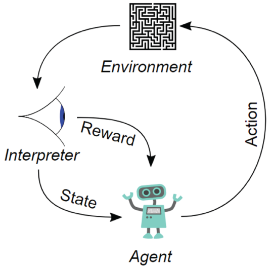
Figure 3.18: A schematic diagram of reinforcement learning, which includes an agent, actions, an environment, a reward, and a state
(Source: https://en.wikipedia.org/wiki/Reinforcement_learning)
Some key terms are often used in reinforcement learning, listed here:
- Environment: Physical world in which the agent operates
- State: Current situation of the agent
- Reward: Positive or negative feedback from the environment
- Policy: The rules that change agent's state to actions
- Value: Future reward that an agent would receive
Q-Learning and SARSA (State-Action-Reward-State-Action) are two commonly used model-free reinforcement learning algorithms. Q-Learning is an off-policy method in which the agent learns the value based on action derived from another policy. SARSA is an on-policy method where it learns the value based on its current action derived from its current policy. These two methods are simple to implement but lack the ability to estimate values for unseen states.
This can be solved by more advanced algorithms such as Deep Q-Networks (DQN) and Deep Deterministic Policy Gradient (DDPG). However, DQNs can handle only discrete, low-dimensional action spaces. DDPG tackles this problem by learning policies in high-dimensional, continuous action spaces.
The following are some practical applications of reinforcement learning:
- Games: Reinforcement learning is widely used for computer games. The best example is Google's AlphaGo, which defeated a world champion in the ancient Chinese game of Go. AlphaGo does not understand the rules of Go; it just learns to play the Go game by trial and error over many times.
- Robotics: Reinforcement learning is also widely used in robotics and industrial automation to enable the robot to create an efficient adaptive control system for itself that learns from its own experience and behavior.
- Natural language processing: Reinforcement learning is used for text summarization engines and dialog agents that can learn from user interactions and improve over time. This is commonly used in healthcare and online stock trading.
The following are a few popular online platforms for reinforcement learning:
- DeepMind Lab: This is an open source 3D game-like platform, created for reinforcement learning simulated environments.
https://deepmind.com/blog/article/open-sourcing-deepmind-lab
- Project Malmo: This is another experimentation platform for reinforcement learning.
https://www.microsoft.com/en-us/research/project/project-malmo/
- OpenAI Gym: This is a toolkit for building and comparing reinforcement learning algorithms.
Q-Learning
Q-learning is one of the most commonly used reinforcement learning algorithms. Let's look at an example to explain how Q-learning works. Take a simple routing example, as shown in Figure 3.19. It contains seven nodes (0–6), called states, and the aim is to choose the best route to go from the Start state (0) to the Goal state (6).
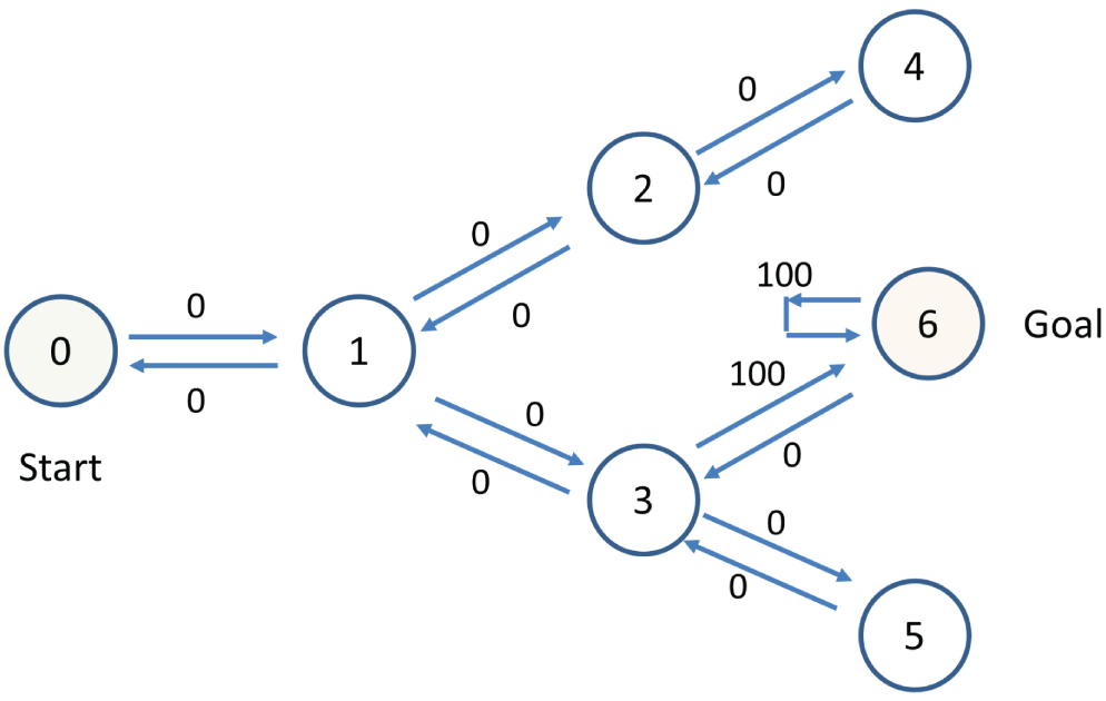
Figure 3.19: A simple routing problem with seven states, with 0 as the start state and 6 as the goal state
Based on Figure 3.19, you can construct a corresponding matrix R, which indicates the reward values from a state to take an action to the next state, as shown in Figure 3.20. The value 0 means it is possible to go from one state to another state, for example, from state 0 to state 1, from state 1 to state 2, and so on. The value -1 means it is not possible, for example, from state 0 to state 3, or from state 2 to state 6, and so on. The value 100 indicates reaching the Goal state; there are only two possibilities, from state 3 to state 6, and from state 6 to state 6.
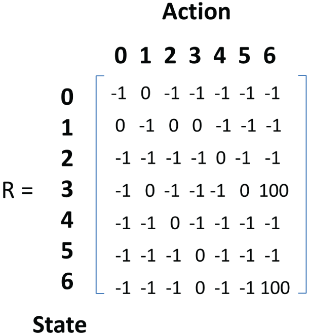
Figure 3.20: The corresponding reward value R matrix of the routing problem
Based on the reward matrix R you can also construct a similar matrix Q, and you update the values of matrix Q iteratively by using the following formula:
where:
| Q(s, a) | is the Q matrix value at state (s) and action (a). |
| R(s, a) | is the R matrix value at state (s) and action (a). |
| is the learning rate. | |
| Q(ns, aa) | is the Q matrix values at next state (ns) and all actions (aa). |
| Max() | is the function to get the maximum values. |
The formula basically says the value of matrix Q at state (s) and action (a) is equal to the sum of the corresponding value in matrix R and the learning parameter ![]() , multiplied by the maximum value of matrix Q for all possible actions in the next state.
, multiplied by the maximum value of matrix Q for all possible actions in the next state.
Example 3.22 shows a simple example of Q-learning for the previous routing problem. It contains two programs, Q_test.py and Q_Utils.py. The following is the Q_test.py program.
The following is the
Q_Utils.py program, which contains the functions needed for Q-learning:
#Example 3.22 - Q_Utils.py#Modified from:#https://amunategui.github.io/reinforcement-learning/index.htmlhttp://firsttimeprogrammer.blogspot.com/2016/09/getting-ai-smarter-with-q-learning.htmlhttp://mnemstudio.org/path-finding-q-learning-tutorial.htmimport numpy as npimport pylab as pltimport networkx as nxdef showgraph(points_list):G=nx.Graph()G.add_edges_from(points_list)pos = nx.spring_layout(G)nx.draw_networkx_nodes(G,pos)nx.draw_networkx_edges(G,pos)nx.draw_networkx_labels(G,pos)plt.show()def createRmat(MATRIX_SIZE,points_list,goal):# create matrix x*yR = np.matrix(np.ones(shape=(MATRIX_SIZE, MATRIX_SIZE)))R *= -1# assign zeros to paths and 100 to goal-reaching pointfor point in points_list:print(point)if point[1] == goal:R[point] = 100else:R[point] = 0if point[0] == goal:R[point[::-1]] = 100else:# reverse of pointR[point[::-1]]= 0# add goal point round tripR[goal,goal]= 100print(R)return Rdef available_actions(R, state):current_state_row = R[state,]av_act = np.where(current_state_row>= 0)[1]return av_actdef sample_next_action(available_act):next_action = int(np.random.choice(available_act,1))return next_actiondef update(R, Q, current_state, action, gamma):max_index = np.where(Q[action,] == np.max(Q[action,]))[1]if max_index.shape[0]> 1:max_index = int(np.random.choice(max_index, size = 1))else:max_index = int(max_index)max_value = Q[action, max_index]Q[current_state, action] = R[current_state, action] + gamma * max_valueprint('max_value', R[current_state, action] + gamma * max_value)if (np.max(Q)> 0):return(np.sum(Q/np.max(Q)*100))else:return (0)
Figure 3.21 and Figure 3.22 show the corresponding outputs of Example 3.22.
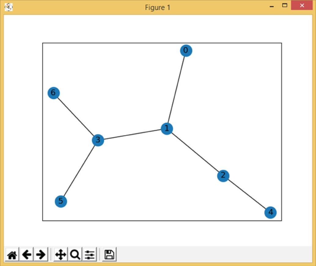
Figure 3.21: The output of Example 3.22, which shows the graph of the network
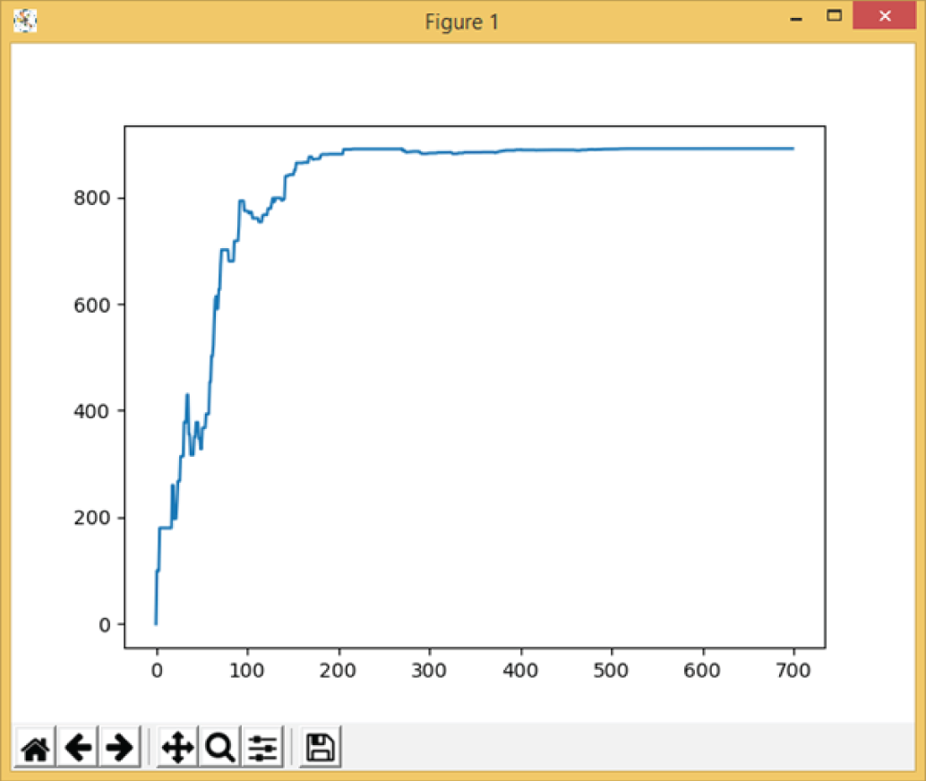
Figure 3.22: The learning process of Example 3.22
The following are the text output of the example, which shows the possible routes from node 0 to node 6, the R matrix with reward values, the training process (mostly omitted), and final trained Q matrix.
Example 3.23 shows a simple program of Python reinforcement learning for balancing a cart pole, using the OpenAI Gym library. Figure 3.23 shows its output.
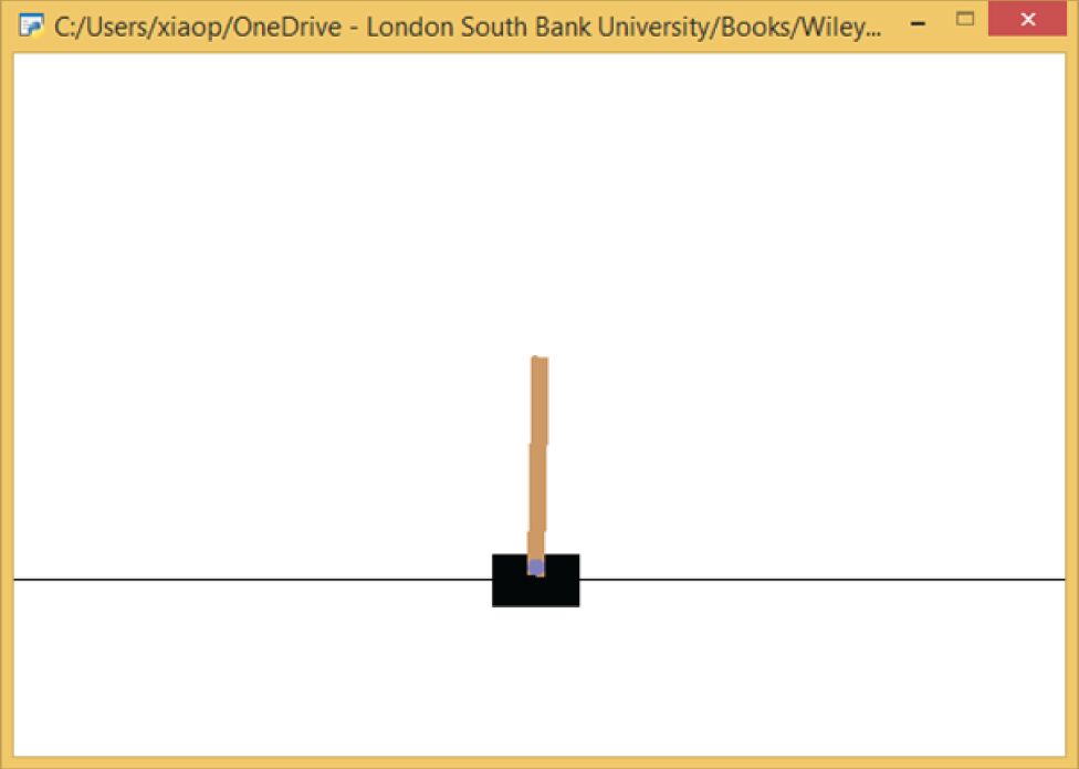
Figure 3.23: The output of Example 3.23, which shows the balancing of a cart pole by using reinforcement learning
3.7 Ensemble Learning
Ensemble learning is a process that uses multiple learning algorithms, or multiple models, to obtain better performance than could be obtained from a single learning algorithm or model. Ensemble learning is mainly used to improve the performance of applications such as classifications, regressions, predictions, and so on.
Two methods are usually used in ensemble learning:
- Averaging methods: In this method, multiple estimators are created independently, and then their predictions are averaged. On average, the combined estimator is usually better than any of the individual base estimators because its variance is reduced. Examples of averaging methods include bagging, forests of randomized trees, and so on.
- Boosting methods: This method builds the base estimators sequentially and tries to reduce the bias of the combined estimator. By combining multiple weak models, it is possible to produce a powerful ensemble. Examples of boosting methods are AdaBoost, gradient tree boosting, and so on.
For more details of ensemble learning in the Scikit-Learn library, visit this page:
https://scikit-learn.org/stable/modules/ensemble.html
Example 3.24 shows a simple program of Python ensemble learning for iris classification. It uses four different classifiers: logistic regression, random forest, naive Bayes, and SVM. It then uses VotingClassifier to choose the best classifier.
The following is the output of the program, which shows the accuracy of each model.
Example 3.25 shows a simple program of Python ensemble learning for diabetes data regression. It first loads the diabetes dataset as X and y, where X contains the values of age, sex, body mass index, average blood pressure, and six blood serum measurements of 442 diabetes patients, and y is the response variable with a range of 25–346; it is a measure of disease progression one year after baseline. It uses four different regressors: gradient boosting, random forest, linear regression, and MLP (neural networks). It then uses VotingRegressor to choose the best regressor. Figure 3.24 shows its output.
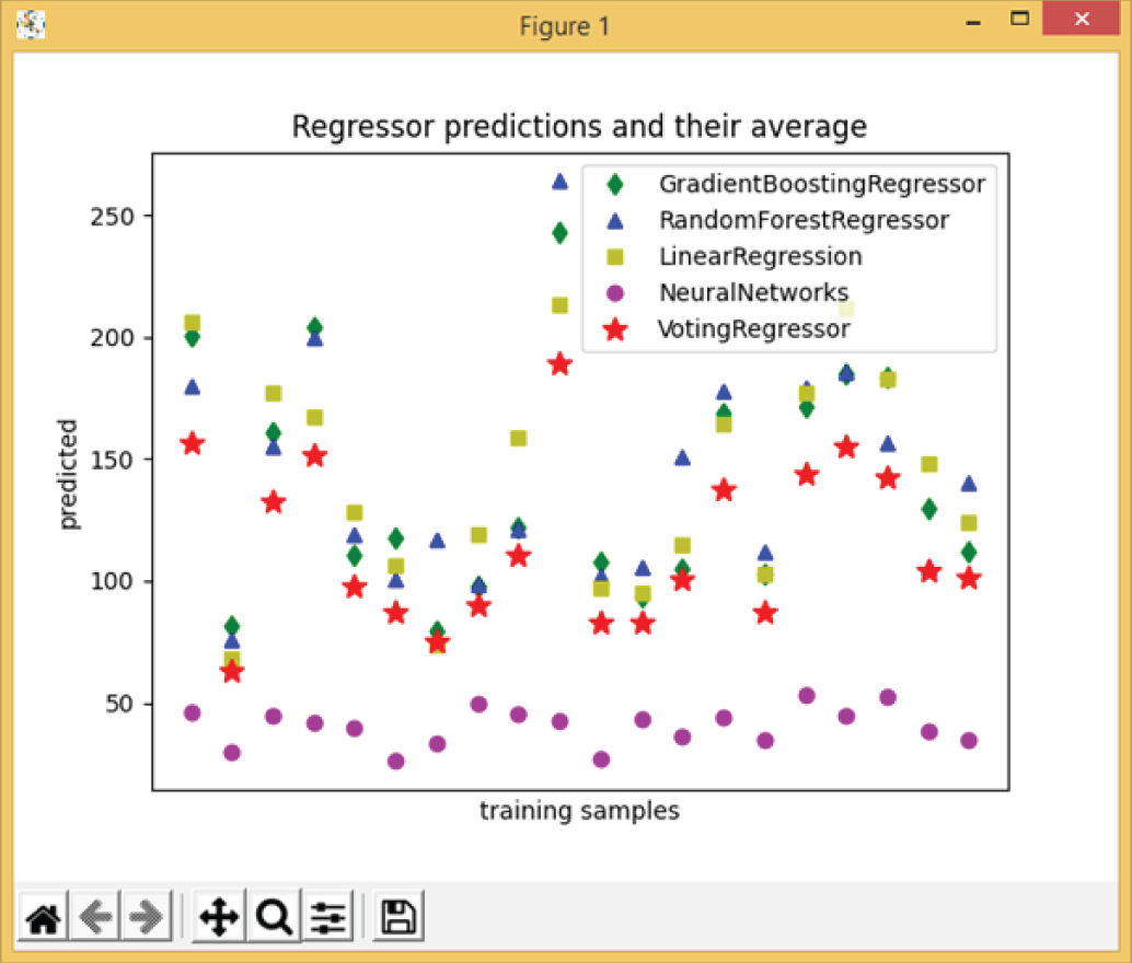
Figure 3.24: The output of Example 3.25, which shows the results of different regression algorithms
3.8 AutoML
Automated machine learning (AutoML) is the process of automating machine learning, from a raw dataset to a deployable model, for easily solving real-world problems. With AutoML, you can use machine learning without having to become an expert in the field.
For more details about AutoML, visit this site:
https://www.automl.org/automl/
There are several AutoML frameworks available, as listed here:
- AutoWEKA is automated machine learning for the WEKA package.
- Auto-sklearn is automated machine learning for the Python Scikit-Learn library.
- TPOT stands for tree-based pipeline optimization tool. It is built on the Scikit-Learn library and optimizes machine learning pipelines using genetic programming.
- H2O AutoML provides automated model selection and ensemble learning for the H2O platform. H2O is an open source, machine learning platform for big data and enterprise applications.
- TransmogrifAI is an AutoML library written in Scala running on the top of Apache Spark.
- MLBoX is an AutoML library with three components: preprocessing, optimization, and prediction.
Let's look at some AutoML example code to demonstrate how to use the AutoML library, called AutoML. You can install the library using the pip command, as shown here:
For more details about the library, check out the following:
https://pypi.org/project/automl/
Example 3.26 shows a simple test program of Python AutoML for Boston housing price regression using the AutoML library.
The following is the output:
3.9 PyCaret
PyCaret is an impressive open source machine learning library in Python that allows you to use multiple models to analyze your data automatically. PyCaret is basically a wrapper around several machine learning libraries such as Scikit-Learn, XGBoost, Microsoft LightGBM, spaCy, and more. PyCaret is a low-code library, and it is best known for its ease of use and efficiency.
To use the PyCaret library, you need to install the library using the pip command, as shown here:
Example 3.27 shows a simple Python PyCaret classification demo program for the iris dataset. It is remarkably simple, requiring only one line of code to set up the classification environment and one line of code to compare all the models.
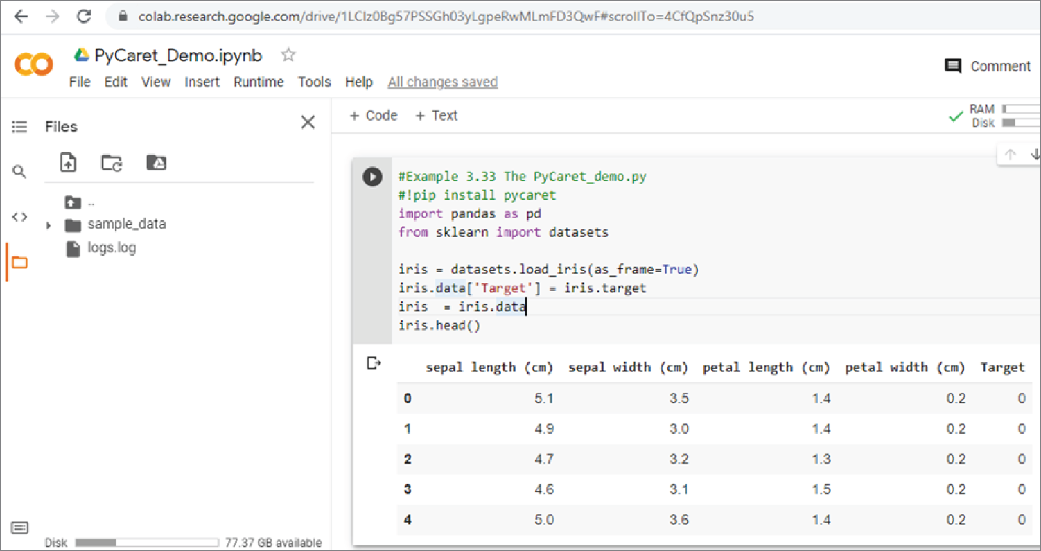
Figure 3.25: The first part of the output of Example 3.27, which shows the Iris dataset
It is easier to run the previous code in Google Colab. Just log in to Google Colab and load the file PyCaret_Demo.ipynb. Figure 3.25 shows the code to load the iris dataset, the code to format it into the required dataframe, and the first five rows of the data. Figure 3.26 shows the code for setting up the classification environment and comparing the models. The results show that linear discriminant analysis gives the best results, with more than 99 percent accuracy.
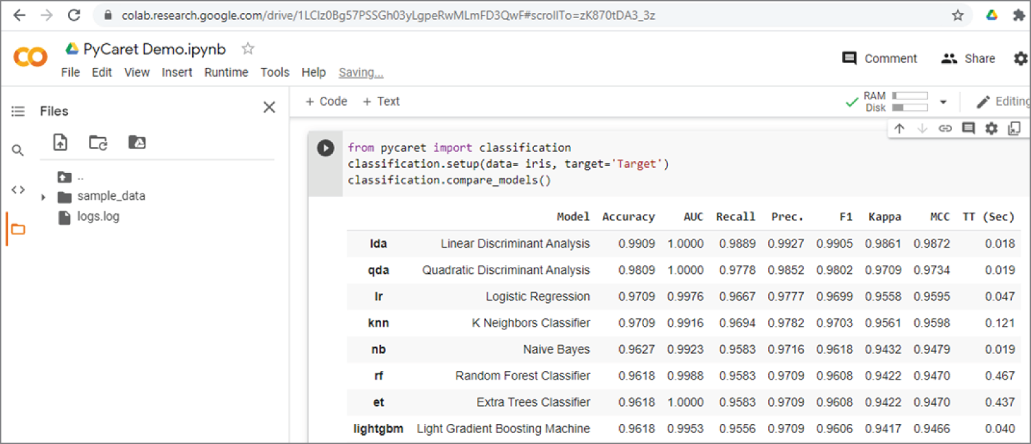
Figure 3.26: The second part of the output of Example 3.27, which shows the results of different regression algorithms
You can use PyCaret for both classification problems and regression problems. For more details about PyCaret, see the following:
3.10 LazyPredict
LazyPredict is another cool library that can perform classification and regression, using a list of algorithms. For more details, see the following:
https://github.com/shankarpandala/lazypredict
To install the LazyPredict library, use this:
Example 3.28 (a, b, c, d and e) is a simple demo example program of Python LazyPredict. Again, it can be easily run on Google Colab. Just go to Google Colab and upload the file called lazypredict.ipynb.
Example 3.28a shows the first section of the code that simply installs the LazyPredict library on Google Colab.
Example 3.28b is the second section of the code that uses the iris dataset as an example to demonstrate the use of LazyPredict for a classifier with the function LazyClassifier(). Again, it is remarkably simple, just one line of code to create the LazyPredict classifier and one line of code to fit and compare the models.
Figure 3.27 shows the Google Colab code of the first two sections of the program. Figure 3.28 shows the output of the second section's classification code. The results show that LabelSpreading gives the best classification results, with 100 percent accuracy!
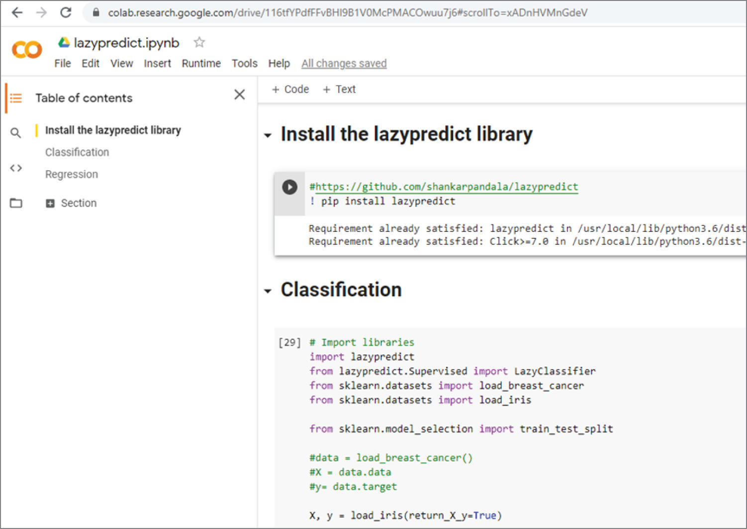
Figure 3.27: The Google Colab code of the first two sections of the program
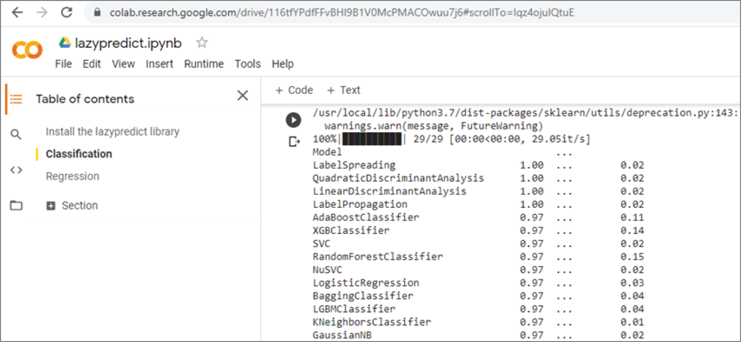
Figure 3.28: The output of the LazyPredict classifier results
Example 3.28c shows the section of code that plots the accuracy of different models. Figure 3.29 shows the output of the plot.
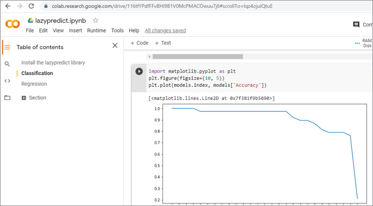
Figure 3.29: The plot of the accuracy of different models
Example 3.28d shows how to use LazyPredict for regression. It uses the California housing price dataset as the example.
Figure 3.30 shows the Google Colab California housing price dataset regression code and output results. The results show that XGBRegressor has the highest R-squared value of 0.84, and GaussianProcessRegressor has the lowest R-squared value of -4467.92.
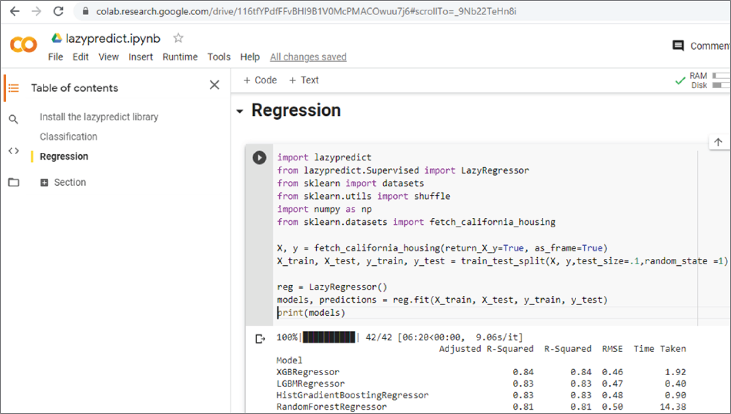
Figure 3.30: Regression code and output results on the Google Colab California housing price dataset
Example 3.28e plots the R-squared values of different models. Figure 3.31 shows the plot of R-squared values of different models.
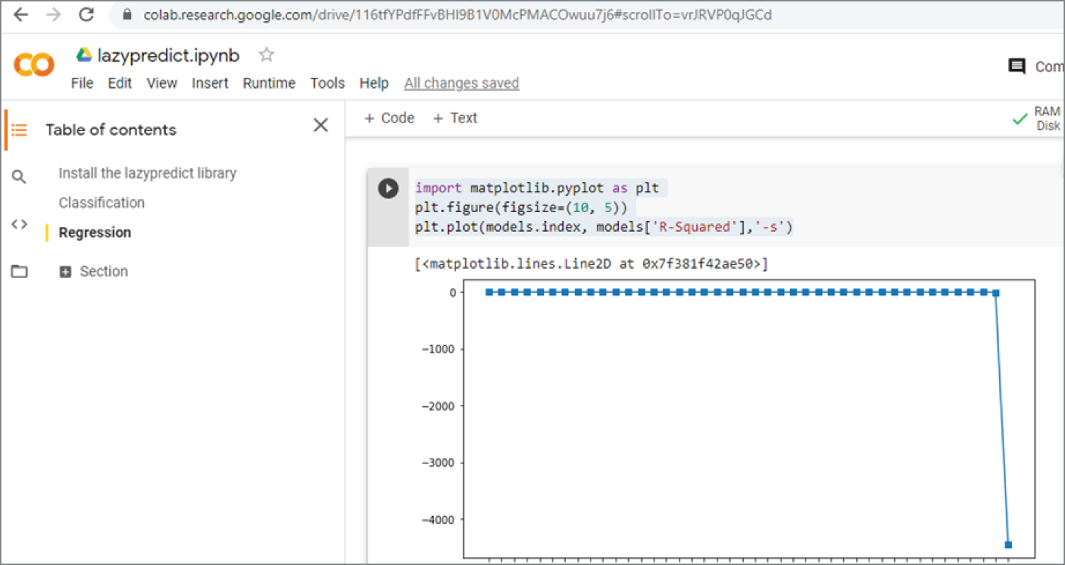
Figure 3.31: The plot of R-Square values of different models
3.11 Summary
This chapter provides a comprehensive overview of machine learning. Machine learning is an important aspect of AI and can be divided into supervised learning, unsupervised learning, semi-supervised learning, and reinforcement learning.
Supervised learning can be generally divided into classification and regression. Classification means predicting the class or category to which the data belongs. Commonly used classification algorithms include support vector machines, naive Bayes, linear discriminant analysis, decision tree, random forest, K-nearest neighbors, neural networks. and so on. Regression means predicting the output values for a given set of input values.
Unsupervised learning is mainly used for clustering data, and K-means clustering is a popular algorithm.
Semi-supervised learning is somewhere between supervised learning and unsupervised learning. Semi-supervised learning is typically used when you have a small amount of labeled data and a large amount of unlabeled data.
Reinforcement learning involves learning in an interactive environment through trial and error using feedback to maximize accumulative rewards. Q-learning is one of the most commonly used reinforcement learning algorithms.
Ensemble learning uses multiple learning algorithms, or multiple models, to obtain better performance than would be possible with a single learning algorithm or model.
AutoML, PyCaret, and LazyPredict are some popular libraries that can automatically use multiple learning algorithms to analyze the data.
3.12 Chapter Review Questions
| Q3.1. | What is machine learning? |
| Q3.2. | What is supervised learning? |
| Q3.3. | What is the difference between classification and regression in supervised learning? |
| Q3.4. | What is SVM? What can it be used for? |
| Q3.5. | What is naive Bayes, and how does it work? |
| Q3.6. | What is linear discriminant analysis, and what is principal component analysis? |
| Q3.7. | What is the difference between decision tree and random forest? |
| Q3.8. | How does K-nearest neighbors work? |
| Q3.9. | What is unsupervised learning? |
| Q3.10. | What is K-means clustering? |
| Q3.11. | What is semi-supervised learning? |
| Q3.12. | What is reinforcement learning, and what can it be used for? |
| Q3.13. | What is Q-learning? |
| Q3.14. | What is ensemble learning? |
| Q3.15. | What are the AutoML, PyCaret, and LazyPredict libraries? |