CHAPTER 4
Deep Learning
“Our intelligence is what makes us human, and AI is an extension of that quality.”
—Yann LeCun (French computer scientist)
CHAPTER OUTLINE
4.1 Introduction
Deep learning (DL) has attracted the world's attention since 2012, when AlexNet won the famous ImageNet challenge. Since then, deep learning has been the hottest research topic in AI. Most of the AI research news you hear today is based on deep learning.
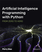
Deep learning is largely considered a subset of machine learning, and it is built on traditional artificial neural networks. As illustrated in Figure 4.1 (left), traditional artificial neural networks typically have one input layer, one output layer, and one hidden layer. The reason they have only one hidden layer is that as the number of hidden layers increases, the complexity also increases, which makes computations unstable and impossible. Deep learning neural networks have an input layer, an output layer, and more than one layer of hidden layers. Deep learning neural networks can have more than one hidden layer due to improved algorithms and higher computing power.
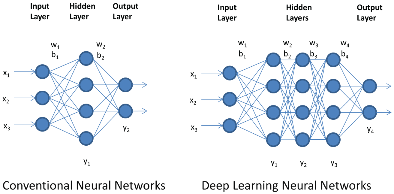
Figure 4.1: Traditional artificial neural networks (left) and deep learning neural networks (right)
Deep learning neural networks can be generally divided into two types:
- Convolutional neural networks
- Recurrent neural networks
Convolutional neural networks are mainly for images, while recurrent neural networks are mainly for sequence data, such as text and time series.
Deep learning can be dated back to 1989, when Yann LeCun and his colleagues proposed a structure for a convolutional neural network, called LeNet. LeNet was successfully used in handwritten digit recognition.
In 2010, Professor Feifei Li of Stanford University created the ImageNet (http://image-net.org/), the largest image database that contains more than 14 million images of daily objects, divided into more than 20,000 categories, such as cats, dogs, cars, tables, chairs, and so on. ImageNet then launched an annual challenge on image classification, called ImageNet Large Scale Visual Recognition Challenge (ILSVRC). The ImageNet challenges only use 1,000 categories. The competitions ran from 2010 to 2017, and moved to Kaggle (https://www.kaggle.com/c/imagenet-object-localization-challenge) after 2017.
The breakthrough came in 2012, when Alex Krizhevsky, Ilya Sutskever, and Geoffrey Hinton from the University of Toronto developed AlexNet. AlexNet won the competition with an impressive top-five accuracy of 85 percent. The next best result was far behind at 74 percent.
In image classification, top-one accuracy is the accuracy with which the best prediction must match the expected answer. Top-five accuracy means that each of the top five answers has the highest probability of matching the expected answer.
The key finding of the original AlexNet publication was that the depth of the model was critical to its high performance. This was computationally expensive but was made feasible by the utilization of graphics processing units (GPUs) during training.
Geoffrey Hinton, Yann LeCun, and Yoshua Bengio, a Canadian computer scientist, are sometimes referred to as the Godfathers of AI or the Godfathers of Deep Learning for their work on deep learning.
In 2014, Christian Szegedy and colleagues at Google achieved top results in object detection with its GoogLeNet model that used the inception module and architecture. This approach was described in its 2014 paper titled “Going Deeper with Convolutions.” GoogLeNet (later known as Inception) becomes the nearest neural network counterpart with a top-five error rate of 6.66 percent. Karen Simonyan and Andrew Zisserman in the Oxford Vision Geometry Group (VGG) achieved top results for image classification and localization with their VGG model. VGG is second place with a top-five error rate of 7.3 percent. The best human-level error rate for classifying ImageNet data is 5.1 percent.
In 2015, Kaiming He and colleagues from Microsoft Research achieved top results in object detection and object detection with localization tasks using their residual network (ResNet). ResNet outperformed human recognition and classified images with a top-five error rate of 3.7 percent.
EfficientNet claims to have achieved a top-five classification accuracy of 97.1 percent in 2019. Figure 4.2 shows the state of the art in image classification on ImageNet, published by Papers with Code.
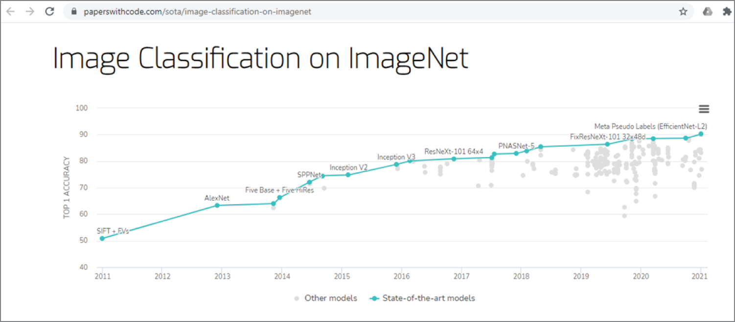
Figure 4.2: The state of the art (SOTA) of image classification on ImageNet
(Source: https://paperswithcode.com/sota/image-classification-on-imagenet)
Figure 4.3 shows typical performances of traditional machine learning algorithms, conventional neural networks (also known as shallow neural networks), and the performance of deep learning neural networks.
Initially, when there is less data, the traditional machine learning algorithms were very efficient and effective. But when the amount of data reaches millions, their performance reaches a plateau, and the performance maintains a stable level even if the data size increases. The traditional neural networks perform better with a larger data set, but still reach a plateau at some point. Only deep learning neural networks continue to increase their performance as data size increases. This is the reason why deep learning neural networks are attracting much research attention.
Figure 4.3: The typical performances of traditional machine learning algorithms, traditional neural networks, and deep learning neural networks against the data
4.2 Artificial Neural Networks
When we talk about deep learning neural networks, we have to start with the traditional neural networks (NNs), which are also called artificial neural networks (ANNs). Traditional neural networks are computer simulations of biological neural networks in the human brain. The concept of neural networks was first developed by American neurophysiologist Warren McCulloch and American logician Walter Pitts in 1943. A biological neural network is a network of interconnected neurons. The biological neuron typically consists of a cell body, dendrites, and an axon. The cell body is also called the soma, while dendrites and axon are filaments that extrude from it. The dendrites typically extrude a few hundred micrometers from the soma, while the axon can be up to a meter long. At the end of the axon are the axon terminals, and each terminal is connected to another neuron by the synapse. For each neuron the dendrites are the inputs from other neurons, and the axon is the output to other neurons. A human brain typically has 100 billion neurons.
There are three types of neurons: sensory neurons respond to stimuli such as touch, sound, or light and send signals to the brain. Motor neurons receive signals from the brain to control muscle. Interneurons connect neurons to other neurons.
Similar to biological neurons, artificial neurons also have an input and an output, as shown in Figure 4.4. Artificial neurons take input signals, multiply them by weights, add them together, and then pass them to a nonlinear activation function for output. The activation function of a node defines the output of that node as a function of an input or a set of inputs. Similar to biological neuron networks, artificial neural networks consist of interconnected artificial neurons. They usually have three layers, as shown in Figure 4.4: an input layer, an output layer, and a hidden layer. The reason they have only one hidden layer is that the computation complexity increases as the number of layers increases.
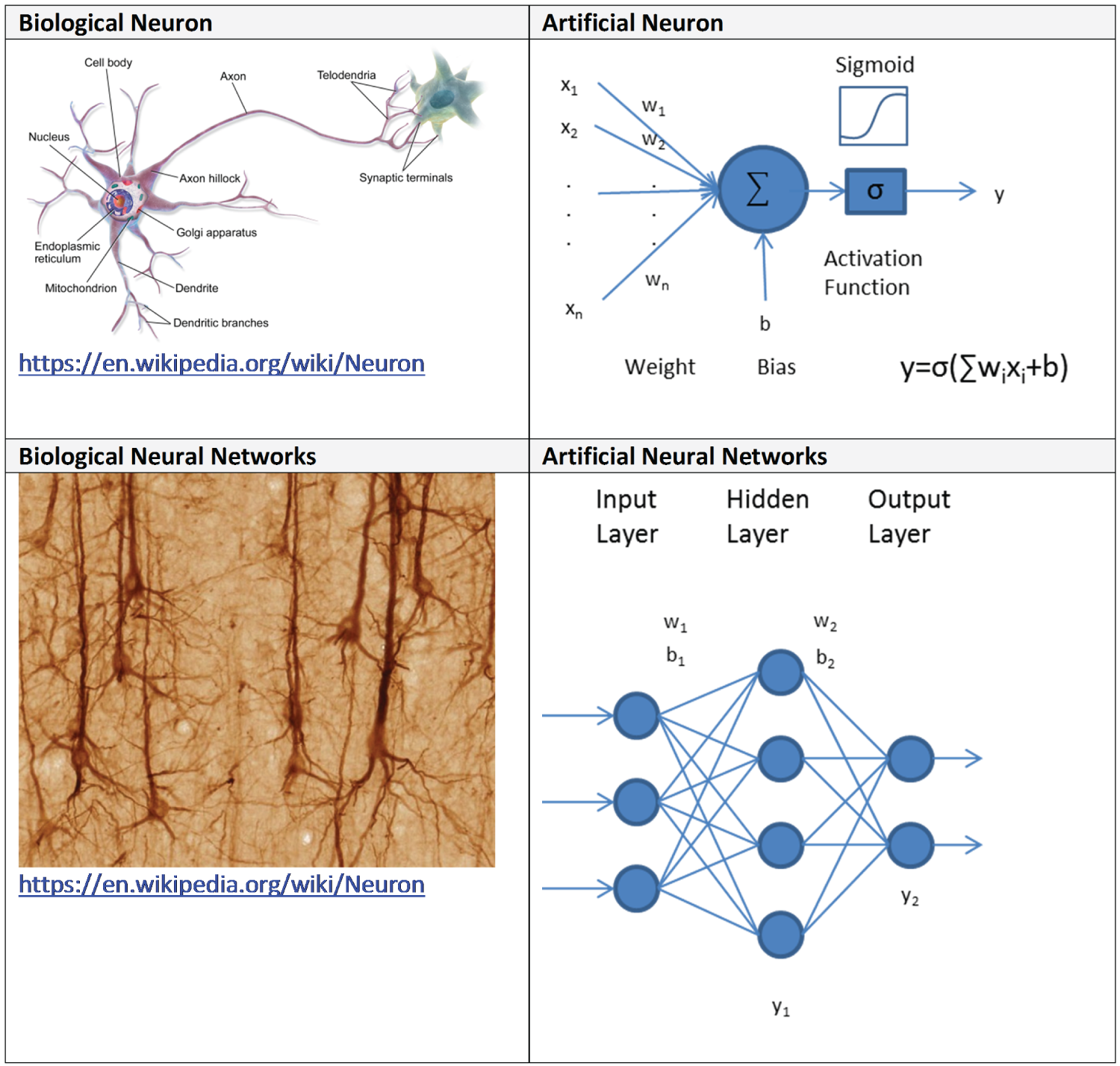
Figure 4.4: Biological neuron versus artificial neuron, and biological neuron networks versus artificial neuron networks
To train an artificial neural network, we first initialize the neural network's weights randomly, and then we feed the network a set of training data, with certain inputs and outputs. Each time the network produces an output from the inputs, it uses a loss function to compare the computed output with the desired output and then returns the differences, called errors, to the network to adjust the weights accordingly. This is called backpropagation, short for “backward propagation of errors.” The weights are adjusted according to the errors using a method called gradient descent, which calculates the gradient of the errors with respect to the neural network weights and adjusts the weights to reduce the errors. This process is then repeated many times until the neural network weights are stabilized. Training an artificial neural network is essentially an optimization problem.
Gradient descent is a commonly used iterative optimization algorithm to find a local minimum of a function. The idea is to take repeated steps in the opposite direction of the gradient, which gives the direction of steepest descent. This is like going down from the top of a mountain and finding a way to explore the bottom. The standard gradient descent follows the path with steepest descent and tends to get stuck at a local minimum. The Stochastic gradient descent is a variant of gradient descent, which solves this problem by adding randomness to the path, as illustrated in Figure 4.5. As a result, stochastic gradient descent converges (reaches the global minimum) much faster than gradient descent.
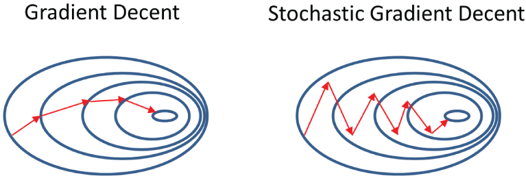
Figure 4.5: The paths of gradient descent and stochastic gradient descent
After training, you can feed the network with a set of unseen data as input, and the network will give you a predicted output. Artificial neural networks usually need a lot of training and take a long time to train, but once trained, they can produce results very quickly.
American psychologist Frank Rosenblatt developed the first artificial neural network called Perceptron in 1958, when he was working at the Cornell Aeronautical Laboratory at Cornell University in Buffalo, New York. Perceptron was an electronic device based on biological neural networks that had a learning capability. The main goal of Perceptron was to recognize different patterns.
Example 4.1 shows a simple Python example with a single neuron. It has two inputs and one output and executes the logic AND of the inputs.
Example 4.2 shows a Python multiple layer perceptron using the Scikit-Learn library. It has two inputs and one output and performs the logical AND of the inputs.
Example 4.3 shows a simple Keras multiple layer perceptron for the breast cancer classification. It has an input layer, a hidden layer (dense layer) of 10 neurons, and an output layer. The dense layer is a neural network layer that each neuron in the dense layer receives input from all neurons of its previous layer.
For more information about traditional neural network, also called multiple layer perceptron, check the following links:
https://scikit-learn.org/stable/modules/neural_networks_supervised.html
https://scikit-neuralnetwork.readthedocs.io/en/latest/module_mlp.html
https://docs.oracle.com/javase/8/docs/technotes/guides/swing/index.html
4.3 Convolutional Neural Networks
The convolutional neural network (CNN, or ConvNet) is probably the most widely used deep learning neural network. CNN is mainly used for image analysis, e.g., image classification, object detection, and image segmentation. It can also be used in recommendation systems, natural language processing, brain-computer interfaces, and financial time series. To date, a number of CNNs have been developed, such as LeNet, AlexNet, GoogLeNet (now Inception), VGG, ResNet, DenseNet, MobileNet, EffecientNet, YOLO, and so on.
Figure 4.6 shows a typical architecture of convolutional neural network that contains an input layer, convolutional layers, pooling layers (subsampling, or down sampling), activation layers, fully connected layers, and an output layer.
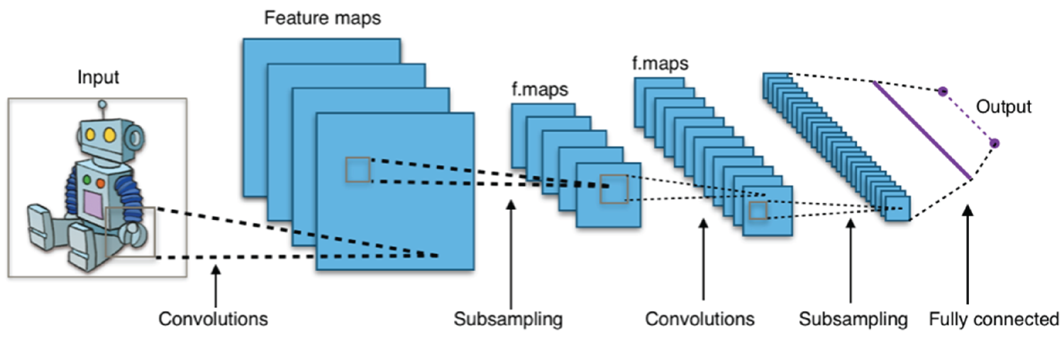
Figure 4.6: Typical convolutional neural network architecture
(Source: https://en.wikipedia.org/wiki/Convolutional_neural_network)
- Input Layer This is the layer that takes images as input. It typically has a size of 32 × 32 × 1 for handwriting digit images in grayscale, and 224 × 224 × 3 for color photo images.
- Convolutional Layer This is the core structure of a convolutional neural network. It uses feature filters (also called kernels) to extra feature information from the input. Figure 4.7a shows some commonly used image filters, or image kernels, that can perform sharpening, blurring, and edge detection of an input image. Figure 4.7b shows the convolution process of an image and a kernel. The convolution process is essentially to multiply the image matrix values with kernel values as an element-wise product and then add all the values to get the convoluted results.
- Pooling Layer Pooling layer is another core structure of CNN. The pooling layer is used for downsampling. Max pooling is the most commonly used pooling. As shown in Figure 4.8, max pooling divides the input image into a series of nonoverlapping rectangles and outputs the maximum for each of these subregions. In this example, a 4 × 48 × 8 image has been mapped by a 2 × 2 window with the stride size of 2. Within the 2 × 2 window, each region (2 × 2) is collapsed into a single pixel by choosing the maximum value. In this way, the entire 4 × 4 image is downsampled into a 2 × 2 image. Another commonly used pooling is average pooling.
- Activation Layer The activation function of a node defines the output of that node as a function of an input or a set of inputs. There are three commonly used activation functions: REctified Linear Unit (ReLU), hyperbolic tangent, and sigmoid function, as shown in Figure 4.9. In deep learning, ReLU is often preferred because it makes neural network training much faster.
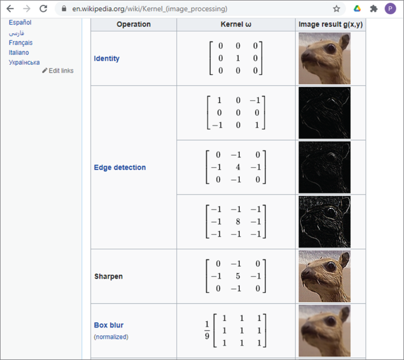
Figure 4.7a: Commonly used image convolution filters (kernels)
(Source:
https://en.wikipedia.org/wiki/Kernel_(image_processing)) - Fully Connected Layer After several convolutional layers and max pooling layers, the high-level reasoning in the neural network is done via fully connected layers. The neurons in a fully connected layer have connections to all activations in the previous layer, as shown in regular (nonconvolutional) artificial neural networks. Fully connected layer is also called dense layer.
- Dropout Layer The dropout layer drops out some of nodes in the neural network to prevent overfitting. Dropout layer can be used with most types of layers, typically after the fully connected layer.
- Output Layer This layer gives the final output of the CNN. For classification, neural networks the number of outputs depends on the number of classes. For regression neural networks, there is only one output that is a floating-point number, a number with a decimal point.
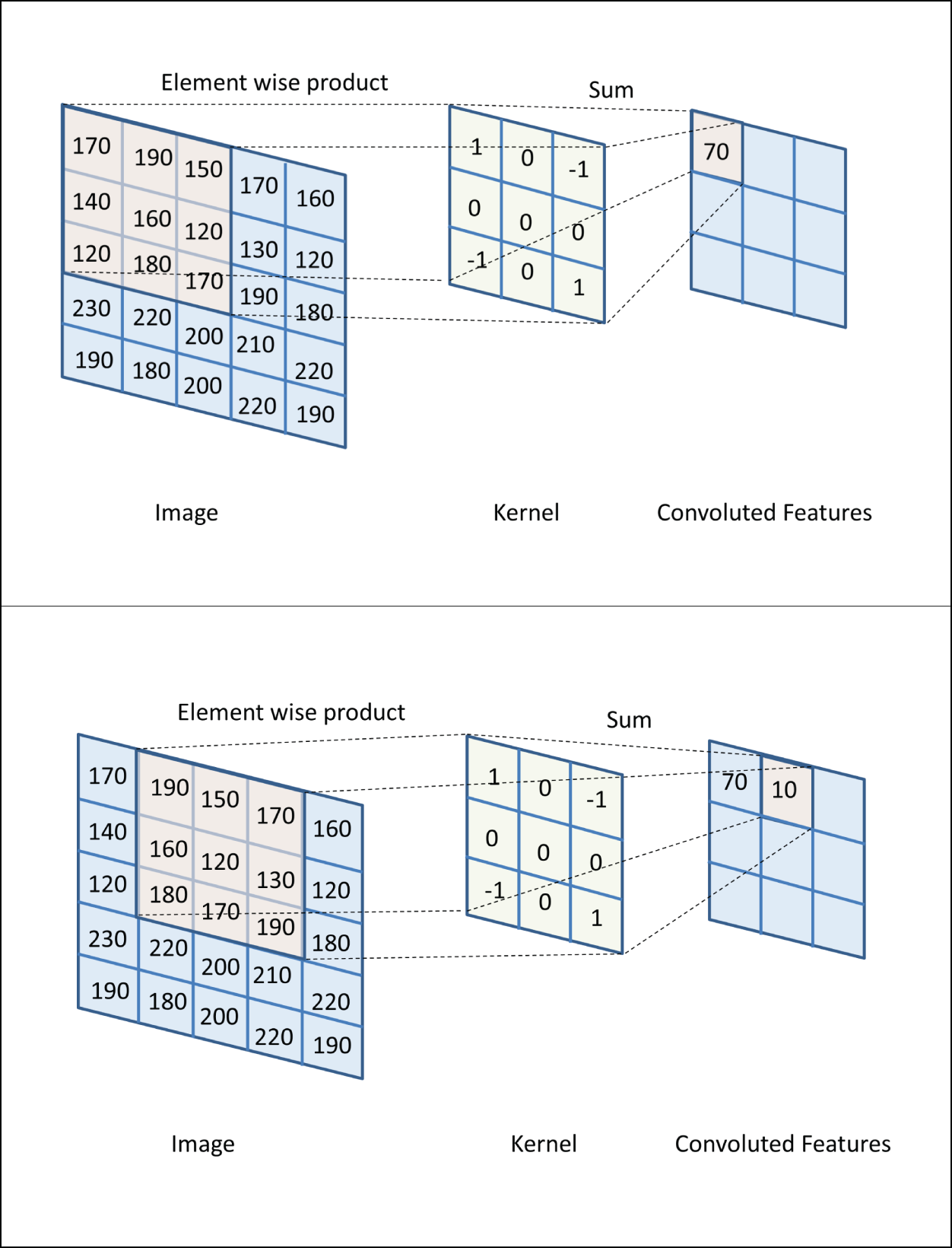
Figure 4.7b: The convolution process of an image and a kernel
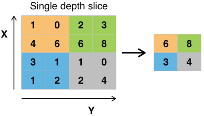
Figure 4.8: Max pooling with a 2×2 filter and stride = 2
(Source: https://en.wikipedia.org/wiki/Convolutional_neural_network)
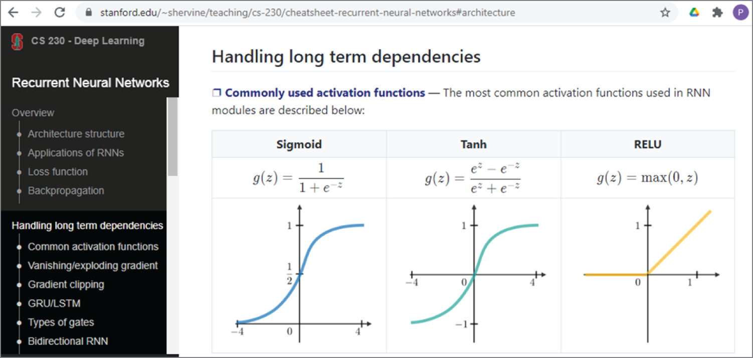
Figure 4.9: Commonly used activation functions
(Source: https://stanford.edu/~shervine/teaching/cs-230/cheatsheet-recurrent-neural-networks#architecture)
The following link shows a simple CNN example implemented with Keras.
4.3.1 LeNet, AlexNet, GoogLeNet
LeNet, often referred to LeNet-5, is probably the best known first convolutional neural network. Developed by Yann LeCun and his colleagues in 1989, LeNet is a seven-layer convolutional neural network. LeNet is famous for classifying handwritten digits, and input images must have the size of 28 (height) × 28 (width) × 1 (channel). See the following LeNet official website details.
http://yann.lecun.com/exdb/lenet/
AlexNet is a convolutional neural network, developed by Alex Krizhevsky in collaboration with Ilya Sutskever and Geoffrey Hinton. Krizhevsky was then a PhD research student of Geoffrey Hinton.
AlexNet made a name for itself when it won the ImageNet Large Scale Visual Recognition Challenge on September 30, 2012. It achieved a top-five error rate of 15.3 percent, more than 10 percentage points lower than the runner-up.
AlexNet has eight layers; the first five were convolutional layers, followed by max-pooling layers, and the last three were fully connected layers. It is divided into two branches, designed for two GPUs. It also uses the nonsaturating ReLU activation function, which showed better training performance than the hyperbolic tangent (Tanh) and sigmoid activation functions. AlexNet has a total of about 61 million parameters and more than 600 million connections.
Figure 4.10 shows the AlexNet architecture from the missinglink.ai website. AlexNet takes input images with the size of 224 (height) × 224 (width) × 3 (channel).
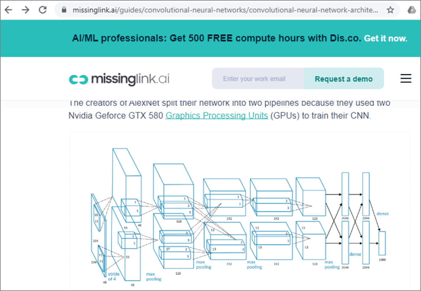
Figure 4.10: The AlexNet architecture from missinglink.ai website
See the following link for the AlexNet original paper, which is considered one of the most influential papers in computer vision. The AlexNet original paper has been cited more than 70,000 times according to Google Scholar.
GoogLeNet, now known as Inception, is another impressive deep learning neural network. Inception v3 is the third edition of Google's Inception convolutional neural network. GoogLeNet takes input images with the size of 224 (height) × 224 (width) × 3 (channel), while Inception takes input images with the size of 299 (height) × 299 (width) × 3 (channel).
Compared to AlexNet, Inception has a concept of Inception modules that perform different-sized convolutions and concatenate the filters for the next layer, as shown in Figure 4.11. Inception v3 has 48 layers and 24 million parameters. Although Inception has more layers than AlexNet, it has many fewer parameters.
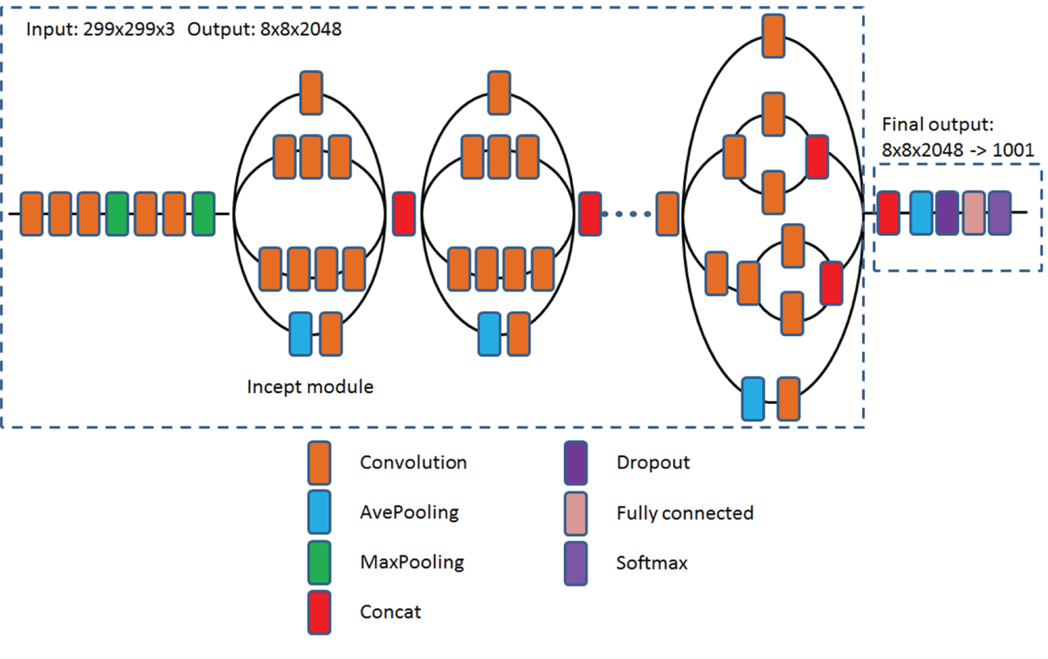
Figure 4.11: The schematic diagram of the Inception v3 architecture
For more details, check the GoogLeNet original paper:
https://static.googleusercontent.com/media/research.google.com/en//pubs/archive/43022.pdf
https://cloud.google.com/tpu/docs/inception-v3-advanced
Example 4.4 shows a Keras implementation of the LeNet-5 deep learning neural network and the output of the summary of the model.
The following is the output:
Example 4.5 shows a Keras implementation of the AlexNet deep learning neural network and the output of the summary of the model.
The following is the output:
Example 4.6 shows a Python code that can load Google Inception V3 and show the summary of the models using the Keras built-in functions. It is just three lines of code!
The following is the truncated output, which shows the first few layers and the last few layers:
Example 4.7 shows a Python code that you can use to create a simple custom-built deep learning neural network and output the summary of the model. It contains an input layer (28, 28, 1), a convolution layer, a max-pooling layer, a dropout layer, a flatten layer, a dense layer, and an output layer. The dense layer is a neural network layer that each neuron in the dense layer receives input from all neurons of its previous layer. The flatten layer flattens the data into a one-dimensional array, which is typically used before the dense layer in convolutional neural networks.
This is the output of the example, showing the summary of the customized neural network:
Example 4.8 shows Python code for loading the MNIST handwriting images and displaying them.
Figure 4.12 shows a few sample images of MNIST handwriting images.
Example 4.9 shows an improved version of the previous code. It creates a simple deep learning neural network, which is used to classify MNIST handwriting digits.
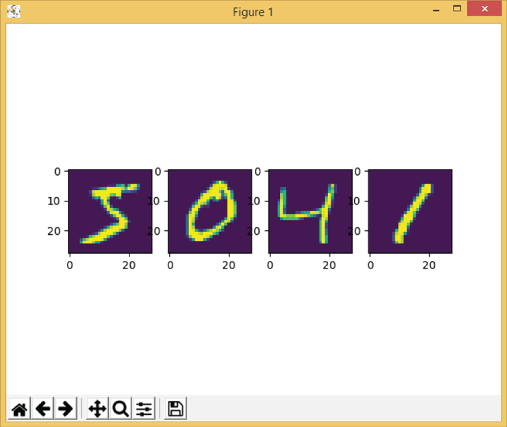
Figure 4.12: The sample images of MNIST handwriting digits images
This is the output of the example, showing the summary of the neural network:
4.3.2 VGG, ResNet, DenseNet, MobileNet, EffecientNet, and YOLO
The VGG deep learning neural network was developed by the Visual Geometry Group at the University of Oxford. There are two versions, VGG 16 and VGG 19. VGG 16 is a 16-layer architecture with a pair of convolutional layers, a pooling layer, and fully connected layer at the end. A VGG network is the idea of much deeper networks and with much smaller filters. A VGG takes input images with the size of 224 (height) × 224 (width) × 3 (channel).
The following link shows an interesting VGG practice website from the University of Oxford, where you can learn to build VGG networks step-by-step using MATLAB software (www.mathworks.com).
https://www.robots.ox.ac.uk/~vgg/practicals/cnn/index.html
Figure 4.13 shows the architecture of VGG16 neural networks. It has an input of 224 × 224 × 3, followed by a convolutional layer and a ReLU layer that reduce the size to 224 × 224 × 64, then to 112 × 112 × 128, 56 × 56 × 256, and finally to 1 × 1 × 1000.
A ResNet (Residual Network) is a convolutional neural network developed by Microsoft. It took the deep learning world by storm in 2015, as the first neural network that could train hundreds or thousands of layers without succumbing to the “vanishing gradient” problem.
ResNet builds on constructs known from pyramidal cells in the cerebral cortex. This is done by utilizing jump connections or shortcuts to skip some layers. Typical ResNet models are implemented with double- or triple-layer jumps that contain nonlinearities (ReLU) and batch normalization in between; see Figure 4.14. ResNet takes input images with the size of 224 (height) × 224 (width) × 3 (channel).
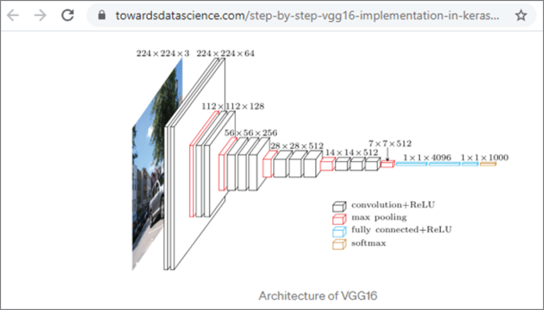
Figure 4.13: The architecture of VGG16 neural networks
(Source: https://towardsdatascience.com/step-by-step-vgg16-implementation-in-keras-for-beginners-a833c686ae6c)
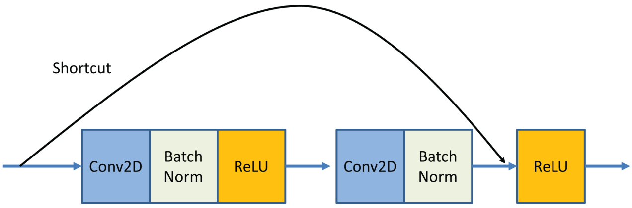
Figure 4.14: The schematic diagram of the ResNet structure with a double layer skip
For more details of ResNet, see the following:
https://arxiv.org/abs/1512.03385v1
https://paperswithcode.com/method/resnet
DenseNet is a convolutional neural network that uses dense connections between layers, where all layers are directly connected; see Figure 4.15. DenseNet has several compelling advantages over other neural networks. It can mitigate the vanishing-gradient problem, enhance feature propagation, promote feature reuse, and significantly reduce the number of parameters. DenseNet takes input images with the size of 224 (height) × 224 (width) × 3 (channel).
For more details of DenseNet, see the following:
https://arxiv.org/abs/1608.06993
https://paperswithcode.com/method/densenet
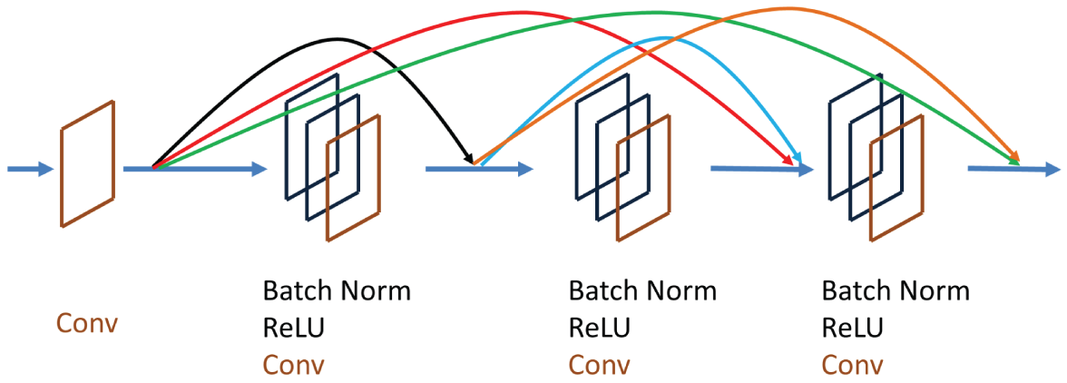
Figure 4.15: The schematic diagram of the DenseNet structure with connections between layers
MobileNet is a family of general-purpose convolutional neural networks designed for use on mobile devices. MobileNet comes in two versions and can be used for image classification, object detection, and more. MobileNets are based on a streamlined architecture for building lightweight deep neural networks. Two simple global hyper-parameters are introduced to find an efficient trade-off between latency and accuracy. These hyper-parameters allow modelers to choose the right model for their applications.
Figure 4.16 shows an overview of MobileNetV1 and the structure of Depthwise Separable Convolution (Light Weight Model). MobileNet takes input images with the size of 224 (height) × 224 (width) × 3 (channel).
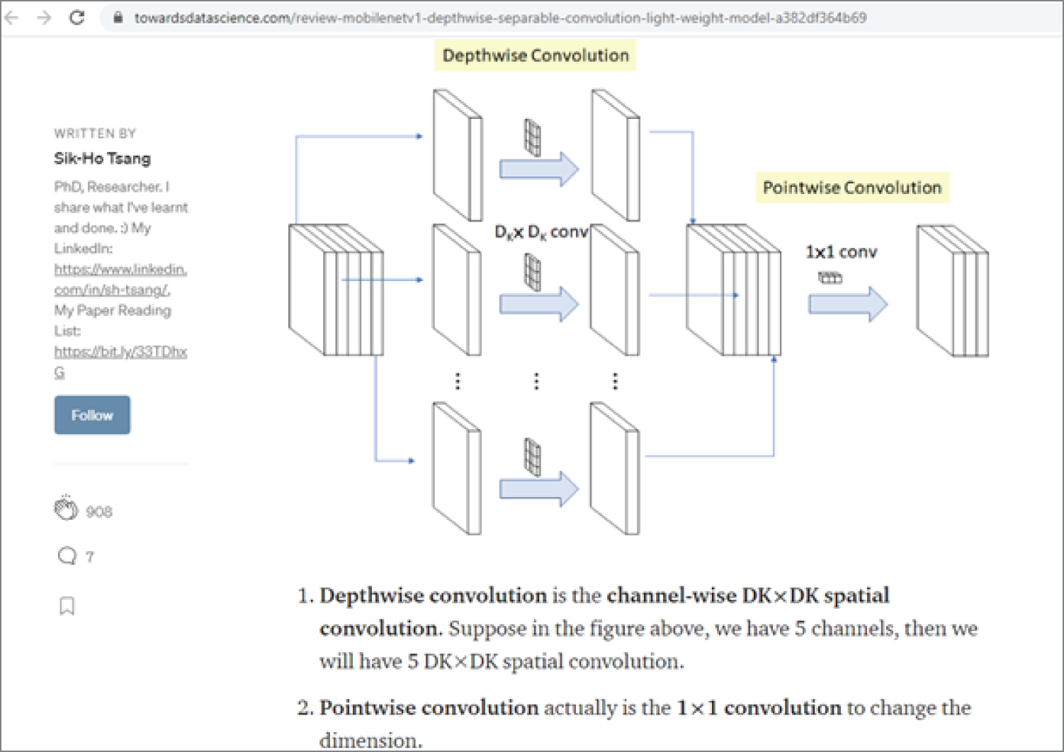
Figure 4.16: Review: MobileNetV1 — Depthwise Separable Convolution (Light Weight Model)
For more details of MobileNet, see the following:
https://arxiv.org/abs/1704.04861
https://ai.googleblog.com/2019/11/introducing-next-generation-on-device.html
https://github.com/tensorflow/models/tree/master/research/slim/nets/mobilenet
EfficientNet is a relatively new deep learning neural network developed by Mingxing Tan, at Google AI, in May 2019. It was developed based on AutoML and Compound Scaling. First, a mobile-size baseline network called EfficientNet-B0 was developed using AutoML MNAS Mobile framework. Then, the compound scaling method was used to scale up this baseline to obtain EfficientNet-B1 to B7. EfficientNet has achieved much better accuracy and efficiency than previous convolutional neural networks. EfficientNet-B7 has achieved a top-one accuracy of 84.3 percent on ImageNet; see Figure 4.17. Efficient takes input images with the size of 224 (height) × 224 (width) × 3 (channel),
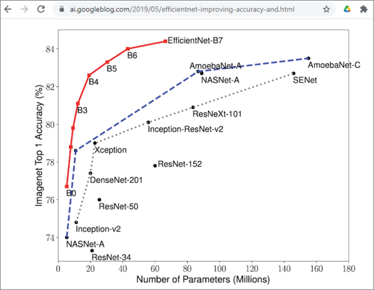
Figure 4.17: Accuracies of different deep learning neural networks on ImageNet
(Source: https://ai.googleblog.com/2019/05/efficientnet-improving-accuracy-and.html)
EfficientNet is also at the top on the ImageNet classification leaderboard, as shown in Figure 4.18.
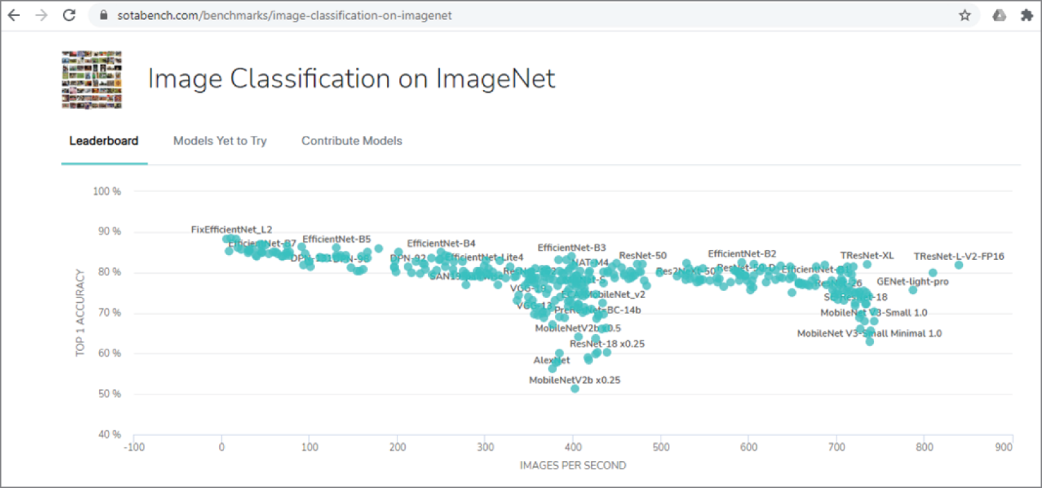
Figure 4.18: The SOTA board for image classification on ImageNet
(Source: https://sotabench.com/benchmarks/image-classification-on-imagenet)
For more details of EfficientNet, see the following:
https://arxiv.org/abs/1905.11946
https://github.com/tensorflow/tpu/tree/master/models/official/efficientnet
YOLO (you only look once) is a state-of-the-art system for real-time object detection. Unlike other convolutional neural networks, YOLO applies a single neural network to the entire image and then divides the image into regions and predicts bounding boxes and probabilities for each region. These bounding boxes are weighted by the predicted probabilities. For more detail, visit the YOLO website:
https://pjreddie.com/darknet/yolo/
Now let's look at some example code.
Example 4.10 shows the Python code for loading a deep learning neural network, such as VGG16, and printing the summary of the model.
This is the output of the example, showing the summary of VGG16 network:
Example 4.11 shows an improved version of the previous example code. In this case, it also uses the model to classify an image.
This is the output of the example, showing the classification results:
Example 4.12 shows a Python code that can load a set of deep learning neural network models, such as VGG16, ResNet50, MobileNet, and Inception V3, display the summary of the models, and use the model to classify an image.
A web camera, or webcam, is a useful tool to capture images to provide data resource for image classification using deep learning. Example 4.13 shows a Python code for image classification based on the image array from a web camera (webcam), using VGG16 deep learning neural network.
Figure 4.19 shows the output of the previous VGG16 classifier based on the images from a webcam, which correctly identifies a computer mouse with 90 percent confidence.
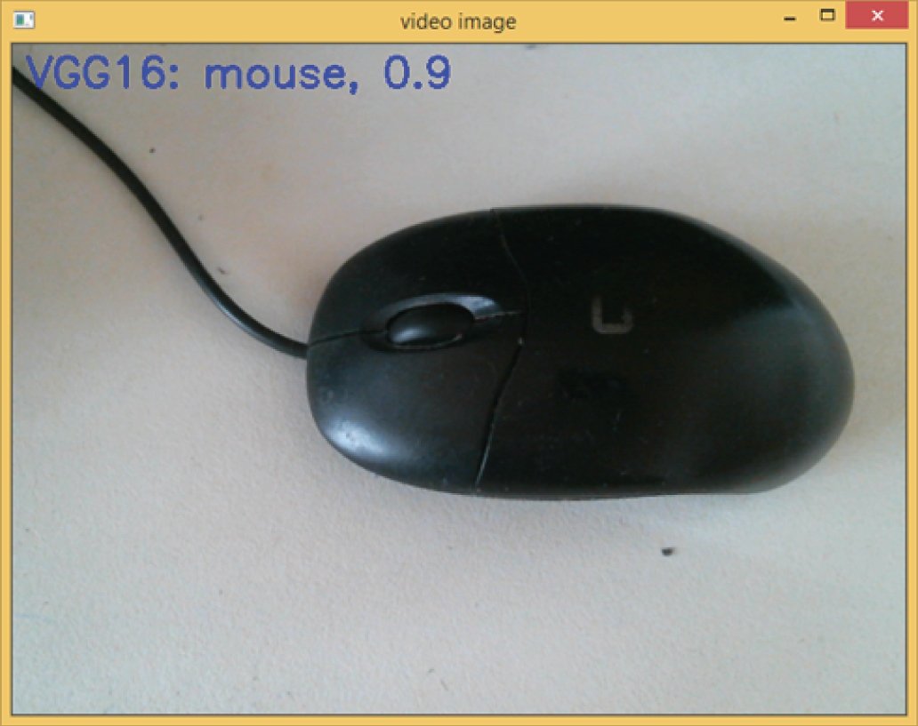
Figure 4.19: The output of VGG16 webcam classification program
Example 4.14 shows a Python code for image classification based on a web camera using different deep learning neural networks such as VGG16, ResNet50, MobileNet, and Google's Inception V3.
The Image-Classifier library is a classification model zoo library that supports 13 different types of deep learning neural networks. It is based on Keras and TensorFlow (https://pypi.org/project/image-classifiers/). To use the library, you must first install it.
Example 4.15 shows a Python code for image classification based on a web camera using Image-Classifier library, which supports a number of different deep learning neural networks such as VGG, ResNet, MobileNet, and Google's Inception, etc.
4.3.3 U-Net
U-Net is a convolutional neural network, developed for biomedical image segmentation at the Computer Vision Group, Department of Computer Science, the University of Freiburg, Germany. Figure 4.20 shows the U-Net website with its architecture.
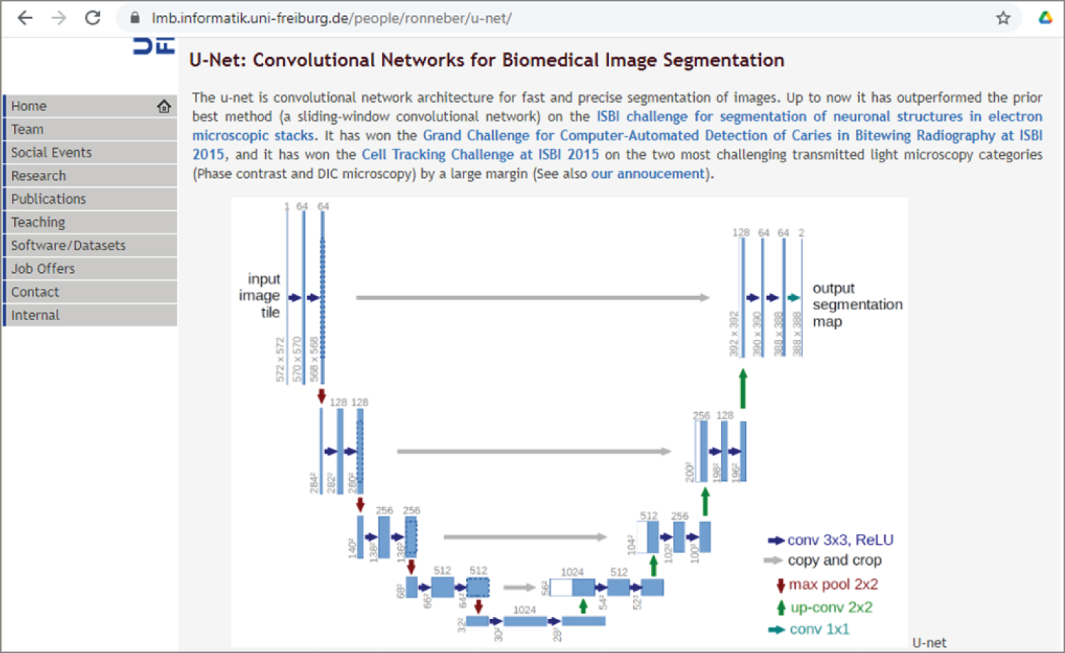
Figure 4.20: The U-Net website at Computer Vision Group, Department of Computer Science, the University of Freiburg, Germany
(Source: https://lmb.informatik.uni-freiburg.de/people/ronneber/u-net/)
U-Net is based on a fully convolutional network and has an input size of 572 × 572. It uses three convolution layers and pooling layers to reduce the input image to a 1,024-feature vector. It then uses three pooling and convolution layers to bring the feature vector back to 382 × 382 as a segmented image. The architecture looks like a U, which is where it gets its name.
To date, U-Net has been used in many applications in biomedical image segmentation, such as brain image segmentation, liver image segmentation, and medical image reconstruction
The easiest way to implement U-Net is to use the Keras-Unet library. See the following links for more details:
https://pypi.org/project/keras-unet/
https://github.com/karolzak/keras-unet
To install the Keras-Unet library, do this:
To create a simple vanilla U-Net model and display a summary of the model, use the following code:
from keras_unet.models import vanilla_unetmodel = vanilla_unet(input_shape=(512, 512, 3))model.summary()
The following is the model summary of a vanilla U-Net. As you can see, the U-Net has changed from the input size (512 × 512 × 3) gradually down to (44 × 44 × 512) and then back up to (324 × 324 × 1).
The following code shows how to plot the U-Net model and save the model into a Portable Network Graphics (PNG) file. Figure 4.21 shows the plot of the U-Net.
from keras.utils import plot_modelplot_model(model, to_file='model.png')
You can also create a customized U-Net model and display the model summary using the following code:
from keras_unet.models import custom:unetmodel = custom:unet(input_shape=(512, 512, 3),use_batch_norm=False,num:classes=1,filters=64,dropout=0.2,output_activation='sigmoid')model.summary()
The quickest way to try image segmentation with the Keras-Unet library is through its GitHub repository. It uses Keras U-Net to segment images from a serial section Transmission Electron Microscopy (ssTEM) dataset of the Drosophila first instar larva ventral nerve cord (VNC), as shown in Figure 4.22.
Just follow the code in this IPython Notebook:
https://github.com/karolzak/keras-unet/blob/master/notebooks/kz-isbi-challenge.ipynb
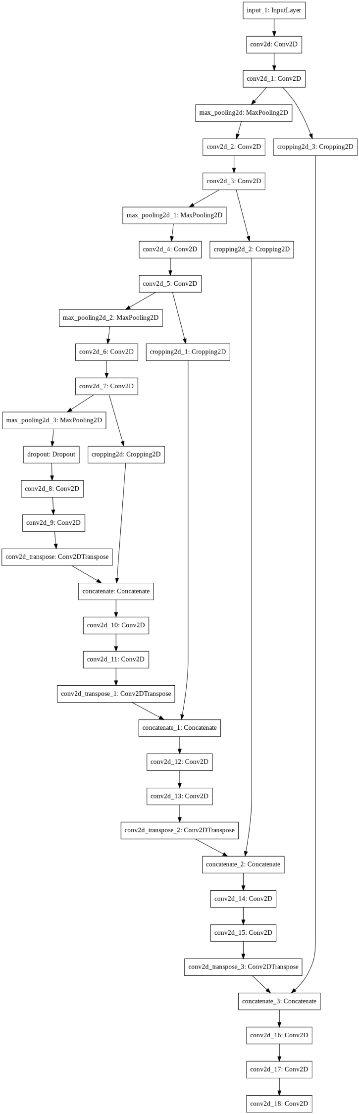
Figure 4.21: The plot of vanilla U-Net model
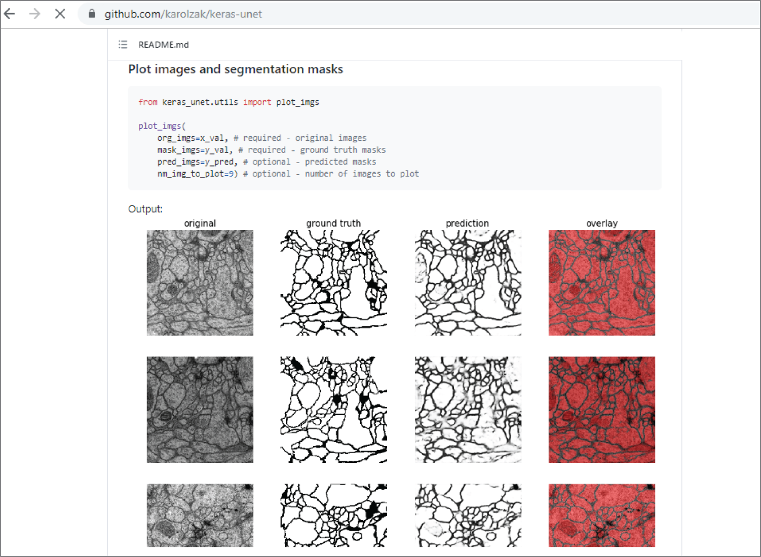
Figure 4.22: The Keras-Unet library GitHub website with serial section Transmission Electron Microscopy images
(Source: https://github.com/karolzak/keras-unet)
The following are more examples of U-Net projects:
https://github.com/zhixuhao/unet
https://github.com/Hsankesara/DeepResearch
https://github.com/devswha/keras-Unet
http://deeplearning.net/tutorial/unet.html
https://www.kaggle.com/phoenigs/u-net-dropout-augmentation-stratification
4.3.4 AutoEncoder
AutoEncoder is a neural network architecture, consisting of two connected networks: Encoder and Decoder, as illustrated in Figure 4.23. The Encoder receives the input image and encodes it into a latent spatial vector of a lower dimension. The network is trained to ignore signal noise during this dimensionality reduction. The Decoder takes this vector and decodes it to produce an output that is as close as possible to the original input. Autoencoders are developed with the goal of learning the low-dimensional feature representations of the input data.
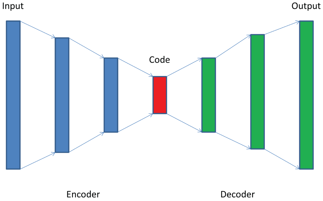
Figure 4.23: The AutoEncoder architecture with two connected networks: Encoder and Decoder
Example 4.16 shows a Python AutoEncoder example code. It was modified based on the example code (https://stackabuse.com/autoencoders-for-image-reconstruction-in-python-and-keras/). It first loads the MNIST handwritten digital images and normalizes the pixel values to 1. Then it builds a simple AutoEncoder that includes a simple encoder and a simple decoder. It then trains the AutoEncoder and uses the trained AutoEncoder to reconstruct the digits.
This is the output of the example, showing the structures of AutoEncoder:
Figure 4.24 shows the example outputs of the AutoEncoder program, which includes the original digit images (left), the output of the encoder called code (middle), and the reconstructed digit images by the decoder.
For more information about AutoEncoders, see the following:
https://blog.keras.io/building-autoencoders-in-keras.html
https://stackabuse.com/autoencoders-for-image-reconstruction-in-python-and-keras/
https://www.analyticsvidhya.com/blog/2020/02/what-is-autoencoder-enhance-image-resolution/
https://www.kaggle.com/shivamb/how-autoencoders-work-intro-and-usecases
https://theaisummer.com/Autoencoder/
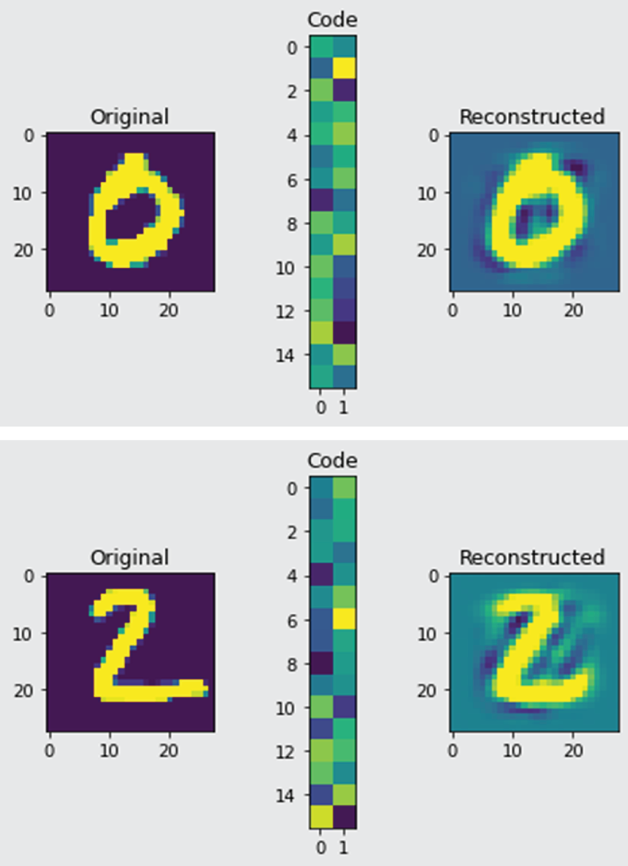
Figure 4.24: The example output of AutoEncoder program, which includes the original digit images (left), the output of the encoder called code (middle), and the reconstructed digit images by decoder (right).
4.3.5 Siamese Neural Networks
When I first started looking into deep learning, one thing always puzzled me. Take image classification, for example. Deep learning neural networks require a large amount of labeled training data to achieve high performance. However, we humans are able to learn things with just a glance at the object. Even if we have never seen passion fruits, we don't need to see thousands and thousands of images before we can recognize them.
Can deep learning neural networks learn the same way? The answer is yes, this is called one-shot learning. In one-shot learning, we need only a single training example for each class instead of training a large set of images. The most commonly used one-shot learning neural network is the Siamese network.
Figure 4.25 shows an interesting introduction of one-shot learning and Siamese networks in Keras. It describes a typical architecture of a convolutional Siamese network as an example of classifying pairs of omniglot images (https://github.com/brendenlake/omniglot). The omniglot data contains 1,623 different handwritten characters from 50 different alphabets.
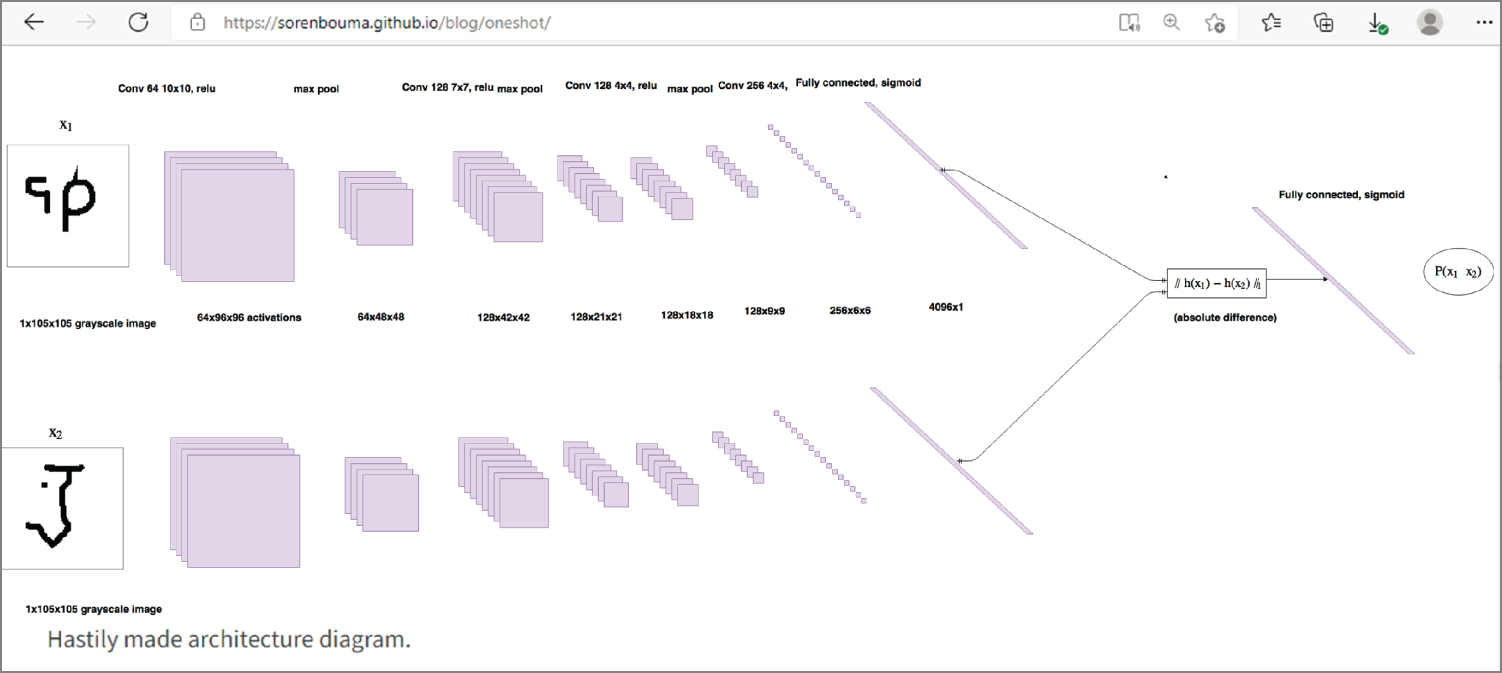
Figure 4.25: One-shot learning and Siamese networks in Keras
The Siamese network contains two convolutional neural networks, called twin neural network. The two neural networks reduce the inputs to lower-dimension tensors; finally, there is a fully connected layer with 4,096 units. The absolute difference between the two vectors is used as input to a linear classifier. A linear classifier performs a classification decision based on the value of a linear combination of the characteristics. The network has 38,951,745 parameters, 96 percent of which belong to the fully connected layer. Training Siamese networks in this way with comparative loss functions can give better performances. Siamese networks have also been used for face recognition.
To try a Siamese network for classifying omniglot images, just follow this interesting IPython notebook:
https://github.com/sorenbouma/keras-oneshot/blob/master/SiameseNet.ipynb
For more information about Siamese networks, visit the following websites:
https://github.com/tensorfreitas/Siamese-Networks-for-One-Shot-Learning
https://towardsdatascience.com/one-shot-learning-with-siamese-networks-using-keras-17f34e75bb3d
https://github.com/hlamba28/One-Shot-Learning-with-Siamese-Networks
https://github.com/akshaysharma096/Siamese-Networks
https://github.com/sorenbouma/keras-oneshot
https://github.com/aspamers/siamese
https://www.cs.cmu.edu/~rsalakhu/papers/oneshot1.pdf
Apart from one-shot learning, there are also few-shot learning and zero-shot learning. Few-shot learning means that the neural network is trained with a few (one to five) images. Zero-shot learning means that the neural network is trained with zero images. This is fascinating! Few-shot learning and zero-shot learning are sometimes categorized as N-shot learning, which means that the neural network is trained with N images.
The key concept of n-shot learning is the prototypical network. Unlike typical deep learning neural networks, prototypical networks do not classify the image directly; instead, they learn the mapping of images in the metric space and group the images into different clusters, called prototypes. In metric space, there is no distinguished “origin” point; instead, you just calculate the distance from one point to another. Prototypical networks then use the distances between prototypes and encoded query images to classify them.
N-shot learning is a learning algorithm that allows the network to learn more with less data. It is typically used when it is hard to find training data, for example, rare diseases, or when the cost of labeling data is too high.
For more details, check the following interesting blog and the GitHub code to the blog:
4.3.6 Capsule Networks
Convolutional neural networks perform best when the image to be classified is similar to the training image dataset. If the image to be classified is different (e.g., rotated, tilted, or transitioned), then the performance drops. Take face detection as an example; if the eyes, nose, and mouth are detected, the image is classified as a face, even if they are in the wrong place. Because of this, there are many shocking errors in image classification.
How can this problem be solved? The answer is a capsule network. A capsule network is a new deep learning network architecture proposed by Sara Sabour, Nicholas Frost, and Geoffrey Hinton in their paper titled “Dynamic Routing Between Capsules” in 2017. See Figure 4.26 for the original paper and a simple three-layer capsule network architecture called CapsNet. In this model, there are modules called capsules that are particularly good at handling different types of visual stimuli such as position, size, orientation, deformation, texture, and so on. As a result, the performance is significantly improved.
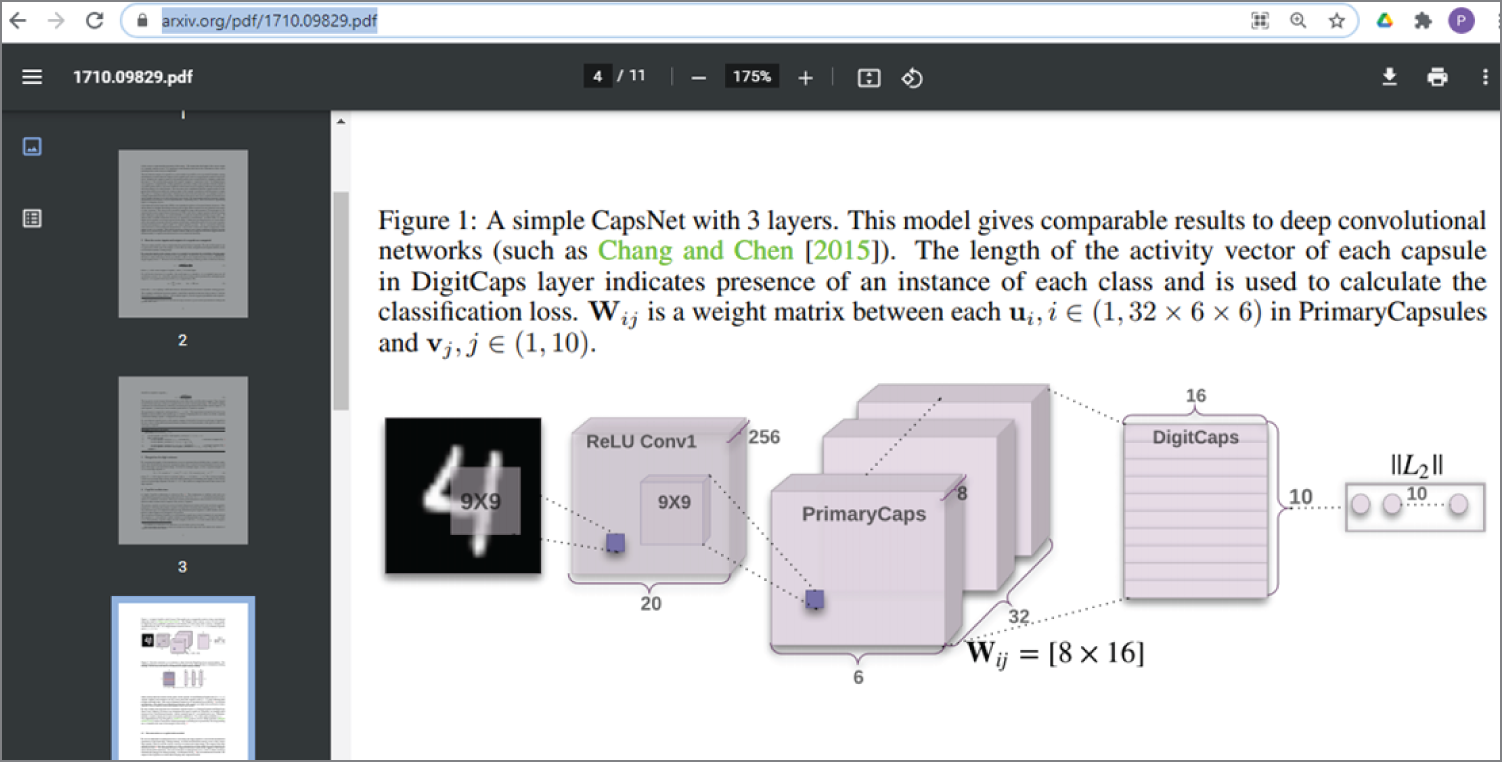
Figure 4.26: The original capsule network paper and a three-layer simple capsule network architecture
(Source: https://arxiv.org/pdf/1710.09829.pdf)
The following website shows an interesting simple introduction of a capsule network, which provides the full capsule network source code implemented in TensorFlow.
https://hackernoon.com/what-is-a-capsnet-or-capsule-network-2bfbe48769cc
This is the corresponding Github site for the source code.
https://github.com/debarko/CapsNet-Tensorflow
The following website shows the capsule network implementation in TensorFlow.
https://github.com/debarko/CapsNet-Tensorflow
Figure 4.27 shows the PyTorch implementation of a capsule graph neural network.
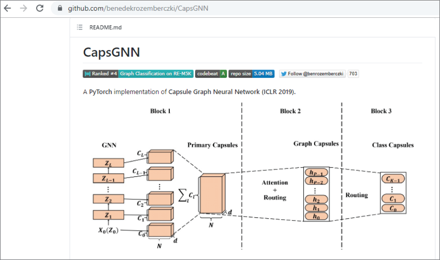
Figure 4.27: A PyTorch implementation of a capsule graph neural network
4.3.7 CNN Layers Visualization
During the development, you may want to see the output of each layer of a convolutional neural network (CNN), whether for debugging purposes or just out of curiosity.
The easiest way to do this is to visualize each layer individually. The following example shows how you can visualize the output of the different convolutional layers in the VGG19 model; it is modified based on an excellent article on visualizing the filters and feature maps in convolutional neural networks (https://machinelearningmastery.com/how-to-visualize-filters-and-feature-maps-in-convolutional-neural-networks/).
We will show the code section by section. You can find the full code in a file called CNN_Visualize_Filters.ipynb. We will run it by uploading it to Google Colab.
Example 4.17 is the first section of the code that shows how to load a VGG19 model and display the summary of the model.
The following is the output that shows the summary of the model:
Example 4.17 shows how to display all the layers in a VGG19 model and show the layer numbers.
The following is the output, showing the layer number and the layer name of all the 25 layers:
The following section of the code shows the filter shape and bias shape for the convolutional layers in the VGG16 model. It uses the function layer.get_weights() to get the filter and bias parameters.
The following output shows all the convolutional layers, their layer number, and their filter and bias parameters. There are 20 convolutional layers. For layer 1, there are 3 color channels; the filter kernel is (3,3), the total number of filters is 64, and total number of bias is also 64.
The following section of the code shows the filters in the first convolutional layers (n = 1) in VGG19 model. Again, the function layer.get_weights() is used to get the filter and bias parameters. Also, the filter is normalized to 0–1 for the purpose of visualization. Then, the first four filters (n_filters, ix = 4, 1) of the total 64 filters are displayed in the first layer.
Figure 4.28 shows the output of the previous code, which shows there are 3 color channels, (3,3) filter size, and total 64 filters in layer 1. It also displays the (3,3) filters in layer 1.
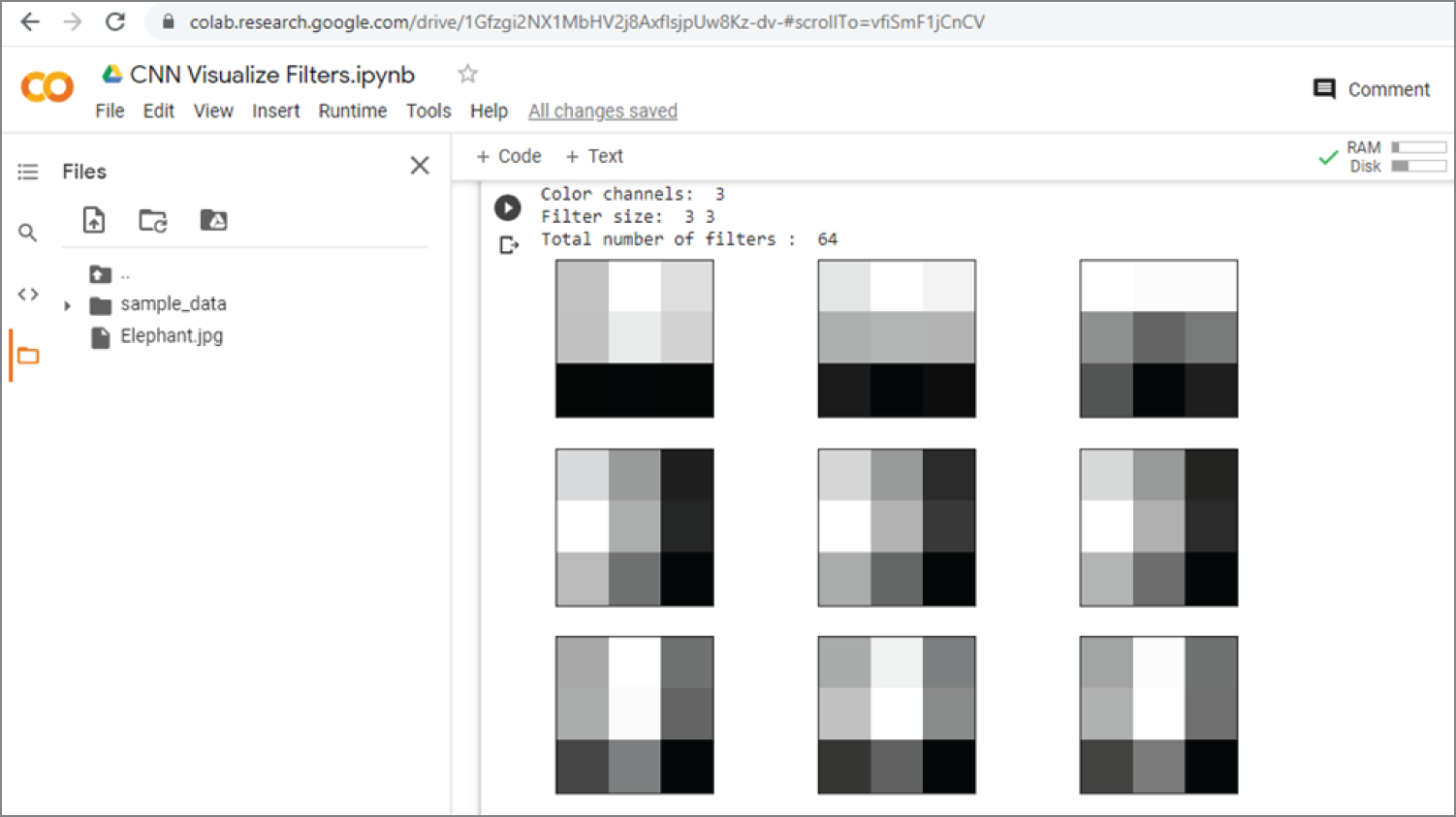
Figure 4.28: The output of the previous example code that displays the filters in layer 1
The following shows a simple function to draw feature maps in a subplot with multiple rows and columns. The number of columns is set to eight, col = 8.
You can visualize the output of the first layer of the VGG19 model by setting the output of layer 1 (n = 1) as the model output; see Model(inputs=model.inputs, outputs=model.layers[n].output) in the following section of the code. Then feature_maps = model.predict(img) is used to get the output of layer 1. We call this layer 1 output as feature maps. Then, it calls plot_feature_maps(feature_maps) to display feature maps. The feature maps basically show what the image looks like after applying all the layer 1 filters. You can change to other layers by changing n = 1.
Figure 4.29 shows the output of the previous code, which shows the structure of the VGG19 model with the first layer as the output. It also shows the feature maps (the output) of layer 1.
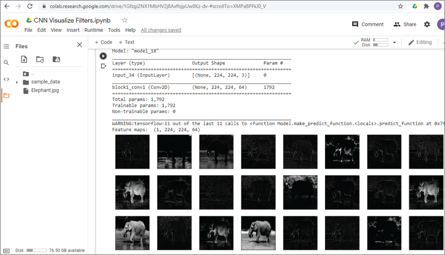
Figure 4.29: The output of the previous code, which shows the structure of the VGG19 model with the first layer as the output. It also shows the feature maps (the output) of layer 1.
Another way to visualize each layer is to use the Keras Visualization Toolkit, see the following link for details.
https://raghakot.github.io/keras-vis/
Figure 4.30 shows the examples of convolution filter visualization, dense layer visualization, and attention maps in Keras Visualization Toolkit.
The following are a few more examples on the visualization of intermediate layers in convolutional neural networks:
https://keras.io/examples/conv_filter_visualization/
https://github.com/JGuillaumin/DeepLearning-NoBlaBla/blob/master/KerasViz.ipynb
https://github.com/gabrielpierobon/cnnshapes/blob/master/README.md
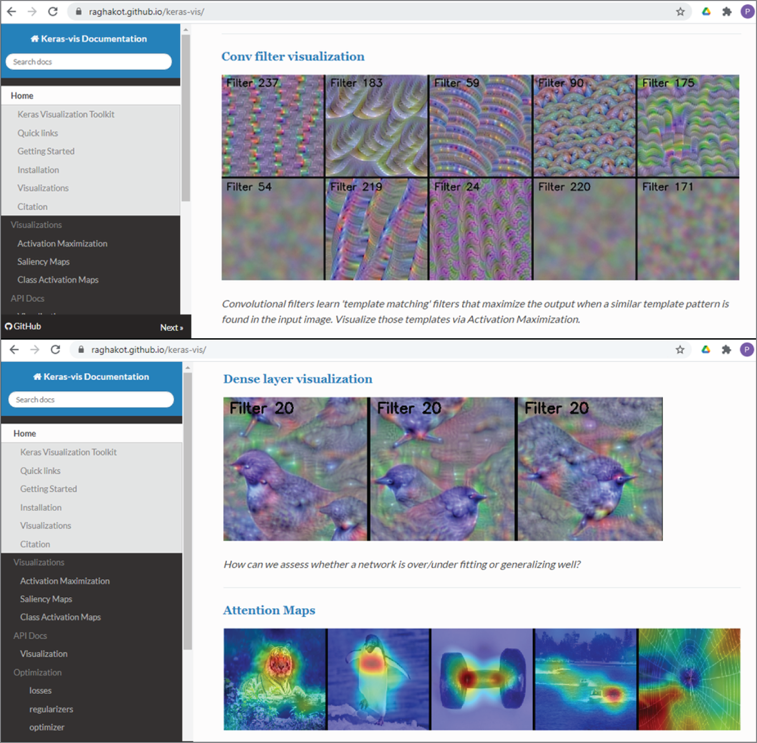
Figure 4.30: The convolutional filter visualization (top), the dense layer visualization, and the attention maps (bottom) in the Keras Visualization Toolkit
(Source: https://raghakot.github.io/keras-vis/)
4.4 Recurrent Neural Networks
Recurrent neural networks (RNNs) are another popular deep learning neural network, along with convolutional neural networks. Convolutional neural networks specialize in processing images, while RNNs specialize in processing sequences. RNNs are derived from feedforward neural networks and can use their internal state (memory) to process variable-length sequences of inputs. RNNs have been applied in sequence prediction, text analysis, and speech recognition.
Figure 4.31 shows the schematic diagram of a recurrent neural network and its unfolded structure. X is the sequential input data, O is the sequential output data, h is the recurrent unit (also called cell), and v is the feedback loop. As shown in Figure 4.31, the recurrent structure occurs repeatedly in the network. The h recurrent unit can be implemented as long short-term memory k (LSTM) network unit and a gated recurrent unit (GRU).
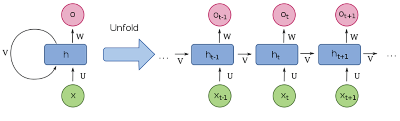
Figure 4.31: The schematic diagram of recurrent neural network and its unfolded structure
(Source: https://en.wikipedia.org/wiki/Recurrent_neural_network)
Figure 4.32 shows an interesting article that explains the differences of RNN, LSTM, and GRU.
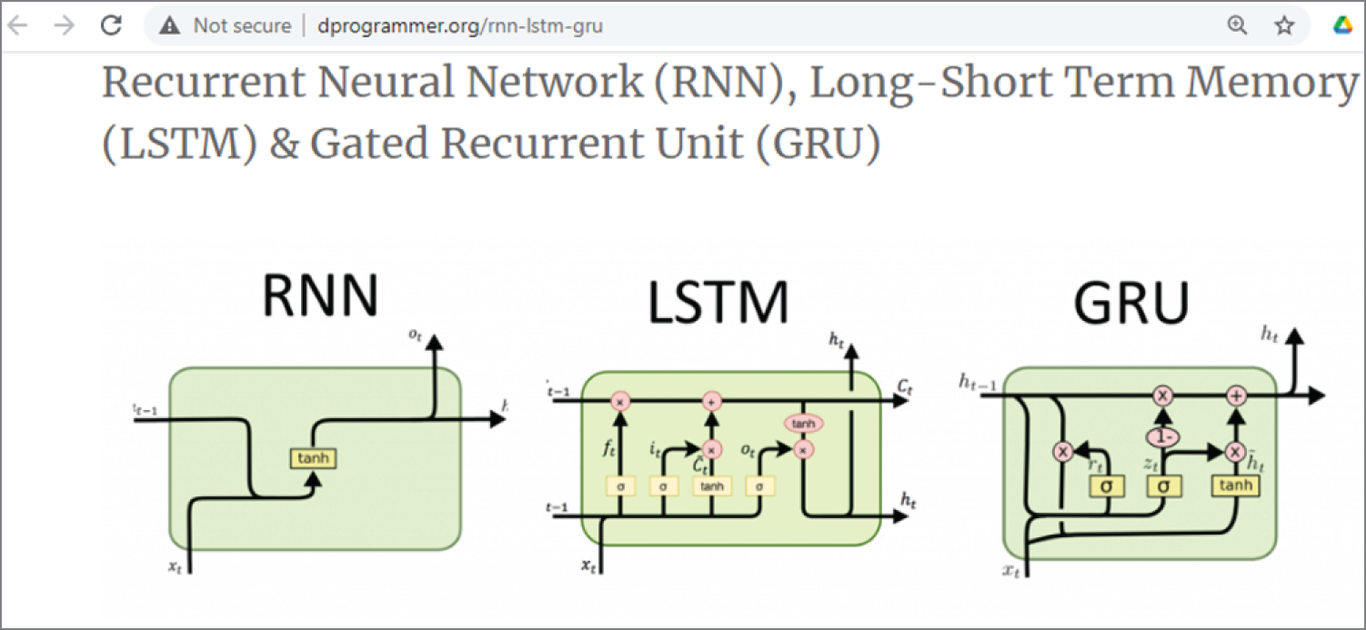
Figure 4.32: The schematic diagram of RNN, LSTM, and GRU
(Source: http://dprogrammer.org/rnn-lstm-gru)
Figure 4.33 shows the four types of recurrent neural networks.
- One to one: One input and one output
- One to many: One input and multiple outputs
- Many to one: Multiple inputs and one output
- Many to many: Multiple inputs and multiple outputs
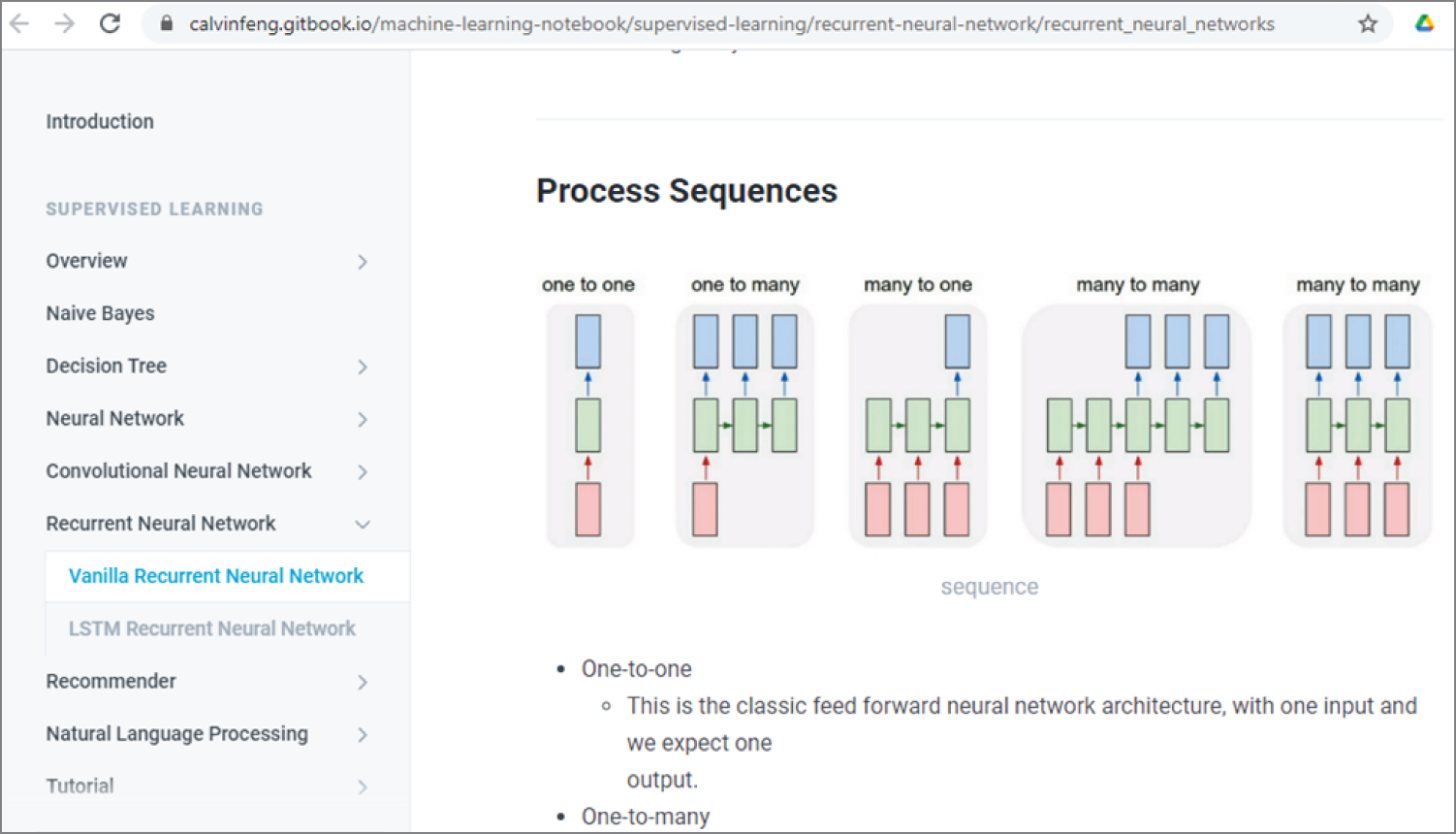
Figure 4.33: The different types of vanilla RNN
For more details about recursive neural networks, see the following:
https://stanford.edu/~shervine/teaching/cs-230/cheatsheet-recurrent-neural-networks
https://www.simplilearn.com/tutorials/deep-learning-tutorial/rnn
4.4.1 Vanilla RNNs
A vanilla RNN is the simplest recurrent neural network that has an input vector, an output vector, and a recurrent unit or cell, as shown in Figure 4.34. Within the recurrent unit, there is an activation function, called tanh. You can also use a different activation function.
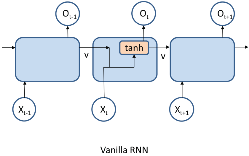
Figure 4.34: The vanilla RNN structure
(Source: https://subscription.packtpub.com/book/data/9781789340990/5/ch05lvl1sec21/vanilla-rnns)
The easiest way to implement vanilla RNN is to use the Keras function called SimpleRNN; see the following links for more details:
https://www.tensorflow.org/api_docs/python/tf/keras/layers/SimpleRNN
https://keras.io/api/layers/recurrent_layers/simple_rnn/
The following is another example of vanilla RNNs using Keras SimpleRNN. It comes from an impressive website called Easy-deep-learning-with-Keras, which contains many illustrative example codes on deep learning neural networks; see Figure 4.35.
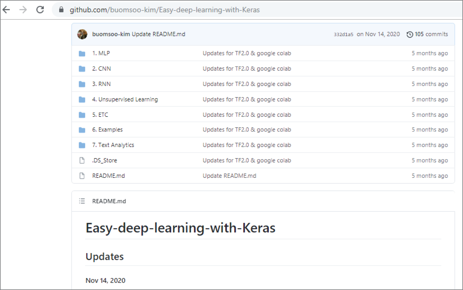
Figure 4.35: The Easy-deep-learning-with-Keras website
(Source: https://github.com/buomsoo-kim/Easy-deep-learning-with-Keras)
4.4.2 Long-Short Term Memory
Long short-term memory (LSTM) is the most popular recurrent neural network architecture. Unlike conventional feedforward neural networks, LSTM has feedback connections. It can process both single input data (e.g., an image) and a sequence of data (e.g., sequences of images in a video). LSTM networks were developed to deal with the vanishing gradient problem and are well-suited for classification and prediction based on time-series data.
Figure 4.36 shows an ordinary LSTM unit, consisting of a cell, an input gate, an output gate, and a forgetting gate. The cell remembers values over arbitrary time intervals, and the three gates regulate the flow of information in and out of the cell.
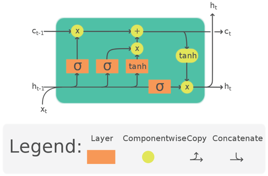
Figure 4.36: The long short memory unit structure
(Source: https://en.wikipedia.org/wiki/Long_short-term:memory)
LSTM has been commonly used in the following:
- Time-series prediction
- Time-series anomaly detection
- Speech recognition
- Language translation
- Music composition
- Text generation
- Handwriting recognition
- Human action recognition
- Robot control
There are five types of LSTM networks:
- LSTM classic
- Peephole connections
- Gated recurrent unit
- Multiplicative LSTM (2017)
- LSTMs with attention
See the following website about the five types of LSTM networks:
https://blog.exxactcorp.com/5-types-lstm-recurrent-neural-network/
Now, let's look at some RNN Python example code. Example 4.18 shows a simple Keras SimpleRNN example.
This is the output of the example, showing the inputs and the outputs of the SimpleRNN:
Example 4.19 is another example of Keras SimpleRNN, showing how to create an RNN model and show the model summary.
This is the output of the previous example, showing the inputs and the outputs of the SimpleRNN:
The following is another Keras SimpleRNN example, predicting the airline passenger numbers, which is modified based on the example code at https://www.datatechnotes.com/2018/12/rnn-example-with-keras-simplernn-in.html.
First, the airline passenger numbers are retrieved from a website:
df = pd.read_csv('https://raw.githubusercontent.com/jbrownlee/Datasets/master/airline-passengers.csv', usecols=[1], engine='python')
Then put the first 80 percent of the data as training data and use the remaining 20 percent for prediction.
Tp = int(df.shape[0]*0.8) Then build a simple RNN model, train the model with the training data (first 80 percent of the total data), predict the data, and finally plot the results.
This is the output of the example, showing the inputs and the outputs of SimpleRNN:
Figure 4.37 shows the output of Example 4.20, showing the original data, the predictions, and the vertical red line representing the 80 percent prediction point. The x-axis consists of data points at different time, and the y-axis consists of the number of air passengers. The predicted result after the 80 percent prediction point agrees well with the original data, even though the model has never seen the data before.
Example 4.21 shows how to create a simple Keras LSTM network. It was modified based on the TensorFlow RNN website (https://www.tensorflow.org/guide/keras/rnn).
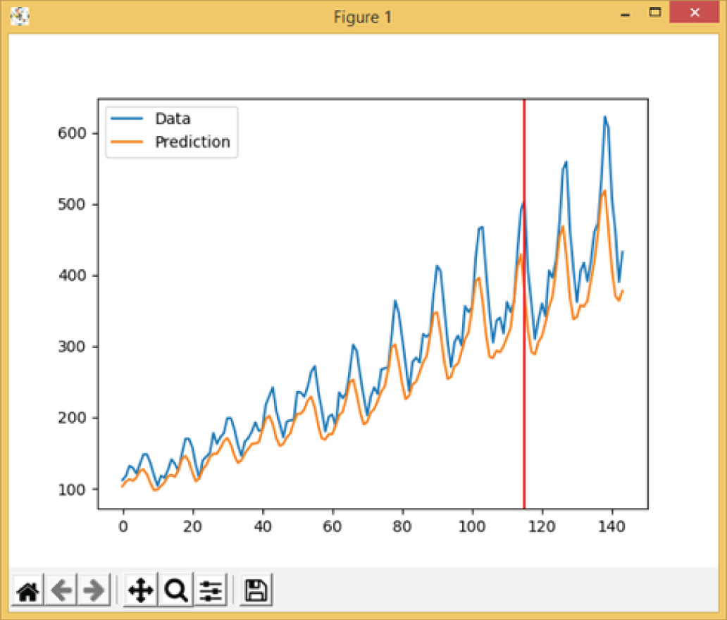
Figure 4.37: The plot output of the Example 4.17
This is the output of the example, showing the summary of the LSTM network:
4.4.3 Natural Language Processing and Python Natural Language Toolkit
Natural language processing (NLP) is a form of artificial intelligence that deals with human (natural) languages, in particular with the processing and analysis of large amounts of natural language data. The main challenges in NPL are speech recognition, natural language understanding, and natural language generation.
The Python Natural Language Toolkit (NLKT) is a leading open source library for natural language processing. It has easy-to-use interfaces with more than 50 corpora lexical resources (such as WordNet). In linguistics, a corpus is a language resource consisting of a large and structured set of texts. NLKT has a number of libraries for classification, tokenization, stemming, tagging, parsing, semantic reasoning, and more.
For more details about NLKT, see the following:
Example 4.22 shows a Python example code for using the NLTK library for text analysis. The text in the code is from the Wikipedia page “Artificial Intelligence” (https://en.wikipedia.org/wiki/Artificial_intelligence).
The following are the outputs of the example, showing the tokens, tags, and entities of the text. This block shows the token entities of the text.
The following block shows the tags entities of the text:
The following block shows the sections of entities of the text:
More examples about natural language processing will be available in Chapter 10.
4.5 Transformers
Transformers are new deep learning neural networks introduced by Hugging Face in 2017, mainly used in the field of natural language processing. Transformers are based on a concept called attention, a mechanism for weighting different parts of the input based on their importance. The creation and development of transformers has demonstrated the effectiveness of large pre-trained models for tackling NLP tasks such as machine translation and question answering. Transformers are starting to make recurrent neural networks obsolete.
Transformers consist of a number of stacked encoders that form the encoder layer, a number of stacked decoders that form the decoder layer, and a bunch of attention layers that form self-attentions and encoder-decoder attentions.
Like recurrent neural networks, transformers are designed to handle sequential data. But, unlike RNNs, transformers do not need to process sequential data in the correct order. For example, if the input data is a natural language sentence, the transformer does not need to process the beginning before the end. Because of this, transformers allow for much more parallelization and thus shorter training time.
The following are the three main types of transformers:
- BERT: Bidirectional Encoder Representations from Transformers
- ALBERT: A Lite BERT
- GPT: Generative Pre-trained Transformer
Transformers have been implemented in both TensorFlow and PyTorch. See the following Transformers GitHub site for details:
https://github.com/huggingface/transformers
4.5.1 BERT and ALBERT
BERT (Bidirectional Encoder Representations from Transformers) is a library for natural language processing. BERT was created and published in 2018 by Jacob Devlin and his colleagues at Google. Google uses BERT to better understand user search queries. The original English-language BERT model used two corpora in pre-training: BookCorpus and English Wikipedia, which together contain around 16GB of uncompressed text.
ALBERT is a “lite” version of BERT. ALBERT uses two parameter-reduction techniques to reduce memory requirements and increase training speed. Google's ALBERT has achieved top scores on three popular benchmark tests for natural language understanding: GLUE, RACE, and SQuAD 2.0. Google has introduced three outstanding innovations with ALBERT: factorized embedding parameterization, cross-layer parameter sharing, and inter-sentence coherence loss. As a result, the large ALBERT model has about 18x fewer parameters compared to BERT-large.
Figure 4.38 shows the performance of the machine on the RACE challenge, where ALBERT has outperformed other models.
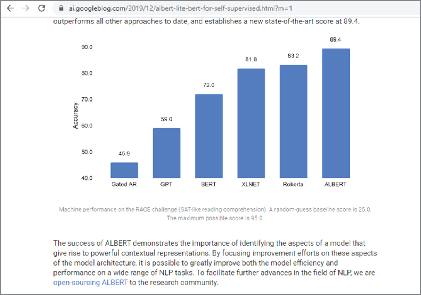
Figure 4.38: The machine performance on the RACE challenge
(Source: https://ai.googleblog.com/2019/12/albert-lite-bert-for-self-supervised.html?m=1)
Example 4.23 shows a Python example code of using transformers for text sentiment analysis.
This is the output of the example, showing the classification result as positive:
Example 4.24 shows a Python example code for using transformers for question answering.
This is the output of the example, showing the answer to the question:
4.5.2 GPT-3
Generative Pre-trained Transformer (GPT) is an autoregressive natural language processing model that uses deep learning neural networks to produce human-like text. GPT was created by OpenAI, a San Francisco–based artificial intelligence research laboratory. There are three versions so far:
- GPT
- GPT-2
- GPT-3
The latest GPT-3 has 175 billion machine learning parameters and has caught the attention of the world in July 2020 with its amazing capabilities. Here is an impressive YouTube video about the GPT-3 demo:
https://www.youtube.com/watch?v=8V20HkoiNtc&t=502s
Before GPT-3, the largest language model was Microsoft's Turing-NLG with 17 billion parameters, released in February 2020.
There are already startups using GPT-3 to provide cool services.
Dover.io allows users to create job descriptions based on simple key words. See the following for more details about the Job Descriptions Creator - Dover.io.
https://www.dover.io/tools/job-description-rewriter
Fitness AI is an iPhone app that uses artificial intelligence to generate personalized workouts. Ask GPT-3 health-related or fitness-related questions for free.
OthersideAI allows users to generate email messages with a list of a few bullet points.
Philosopher AI allows users to ask philosophical questions. You need to pay for the service.
CopyAI helps users to automatically generate professional marketing copy based on your input. It claims to be able to automate the tedious and often frustrating aspects of copy creation.
4.5.3 Switch Transformers
In early 2021, researchers at Google Brain developed a new, open source AI model for NLP, called Switch Transformer, which has a whopping 1.6T parameters, nearly ten times that of GPT-3. The training speed of Switch Transformer has also been improved by seven times compared to previous architectures.
Switch Transformer uses a switch feed-forward neural network (FFN) layer to replace the standard FFN layer in the transformer architecture. Instead of a single FFN, each switch layer contains multiple FFNs, called experts. The Switch Transformer architecture is based on the concept of Mixture of Experts (MoE). This approach simplifies the computations and reduces the communication cost.
At the time of writing this book, Google has not released the pretrained model weights for Switch Transformer; for more details about Switch Transformer, visit the following:
https://arxiv.org/abs/2101.03961
https://github.com/tensorflow/mesh/blob/master/mesh_tensorflow/transformer/
4.6 Graph Neural Networks
Although recurrent neural networks have been superseded by transformers in natural language processing, they are still useful in many areas that require sequential decision-making and in reinforcement learning. Recurrent neural networks typically take input data in a sequence, such as time-series data or language text. A graph neural network (GNN) is a special type of recurrent neural network that can take graphs as input data. GNN has been used in many applications such as analyzing social media data, and molecular structures. There is also the quantum graph neural networks (QGNNs) for quantum chemistry analysis. QGNNs have been applied to learning quantum dynamics, graph clustering, and graph isomorphism classification.
Convolutional neural networks work well on data with a regular grid structure, such as images, but not on graphs because they are arbitrarily large and have a complex topology.
The following website shows a friendly introduction to the GNN. It also covers the future of GNN including Quantum Graph Neural Networks (QGNNs).
https://www.kdnuggets.com/2020/11/friendly-introduction-graph-neural-networks.html
The following website shows the introduction to a GNN and its applications, such as modeling real-world physical systems, molecular fingerprints, protein interface prediction, modeling social interactions, and so on.
https://neptune.ai/blog/graph-neural-network-and-some-of-gnn-applications
The following is a GNN implementation by Google's DeepMind:
https://github.com/deepmind/graph_nets
The following is a GNN implementation by Facebook's PyTorch:
https://github.com/rusty1s/pytorch_geometric
For more details about GNNs, visit the following website:
https://theaisummer.com/Graph_Neural_Networks/
4.6.1 SuperGLUE
SuperGlue is a CVPR 2020 research project, being conducted at Magic Leap. CVPR (Conference on Computer Vision and Pattern Recognition) is the premier annual event on computer vision, including several co-located workshops and short courses in addition to the main conference. The SuperGlue network is a GNN combined with an optimal matching layer that is trained to match two sets of sparse image features. This repo includes PyTorch code and pre-trained weights for running the SuperGlue matching network based on SuperPoint key points and descriptors. Given a pair of images, you can use this repo to extract matching features for the image pair. See the following links for details.
4.7 Bayesian Neural Networks
Traditional deep learning neural networks have a fixed value for their parameters; hence, they are also called deterministic neural networks. Traditional deep learning neural networks have been successful in many applications. However, they also have some drawbacks. For example, mere knowledge of the input-output mapping is inadequate when it comes to generating predictive uncertainty in their predictions. This can be important when the available data is limited or the data does not span the whole space of interest.
Bayesian neural networks (BNNs) have been developed to address these issues. Bayesian neural networks are neural networks whose weights or parameters are expressed as a distribution rather than a deterministic value and are learned using Bayesian inference. The output of Bayesian neural networks is also a distribution rather than a fixed value.
Figure 4.39 shows the differences between traditional neural networks and Bayesian neural networks.

Figure 4.39: The traditional neural networks and Bayesian neural networks
The following is the Keras website on probabilistic Bayesian neural networks, providing a detailed introduction and a Google Colab IPython Notebook with the source code. You can access the code by clicking the View in Colab link.
https://keras.io/examples/keras_recipes/bayesian_neural_networks/
Figure 4.40 shows the modified version of the Google Colab code. You can access the modified code by using the following link or by uploading a file named
Copy_of_bayesian_neural_networks_wine.ipynb to your Google Colab.
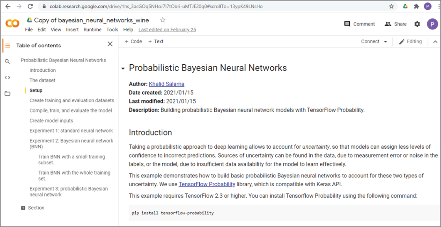
Figure 4.40: The corresponding Google Colab code for the Keras website on probabilistic Bayesian neural networks
(Source: https://colab.research.google.com/drive/1hs_3acGOq5NHoJ7l7tObri-uMTJE20q0#scrollTo=13ypK49LNsHo)
The modified code performs three experiments to predict wine quality.
- Experiment 1: standard neural network
In this experiment, the basic deterministic model is used to predict the wine quality. From the following outputs, you can see that only one fixed value is predicted for each input:
- Experiment 2: Bayesian neural network (BNN)
In this experiment, the Bayesian neural network model is used to predict wine quality. The following outputs show that for each input a mean value, a minimum value, and a maximum value are predicted:
- Experiment 3: Probabilistic Bayesian neural network
This experiment uses the probabilistic Bayesian neural network model to predict wine quality. The following is the output. As you can see, the output is now a distribution, including the mean, the variance, and the confidence intervals (CI) of the prediction.
You can also plot the mean, the maximum, and the minimum on a graph. Figure 4.41 shows the code for plotting the mean, the maximum, and the minimum of the predictions (top), and the corresponding plot (bottom).
The following is a list of interesting tutorials and projects about Bayesian neural networks:
https://github.com/JavierAntoran/Bayesian-Neural-Networks
https://davidstutz.de/a-short-introduction-to-bayesian-neural-networks/
https://sanjaykthakur.com/2018/12/05/the-very-basics-of-bayesian-neural-networks/
http://edwardlib.org/tutorials/bayesian-neural-network
http://krasserm.github.io/2019/03/14/bayesian-neural-networks/
https://github.com/krasserm/bayesian-machine-learning
https://inferpy.readthedocs.io/en/0.0.3/notes/guidebayesian.html
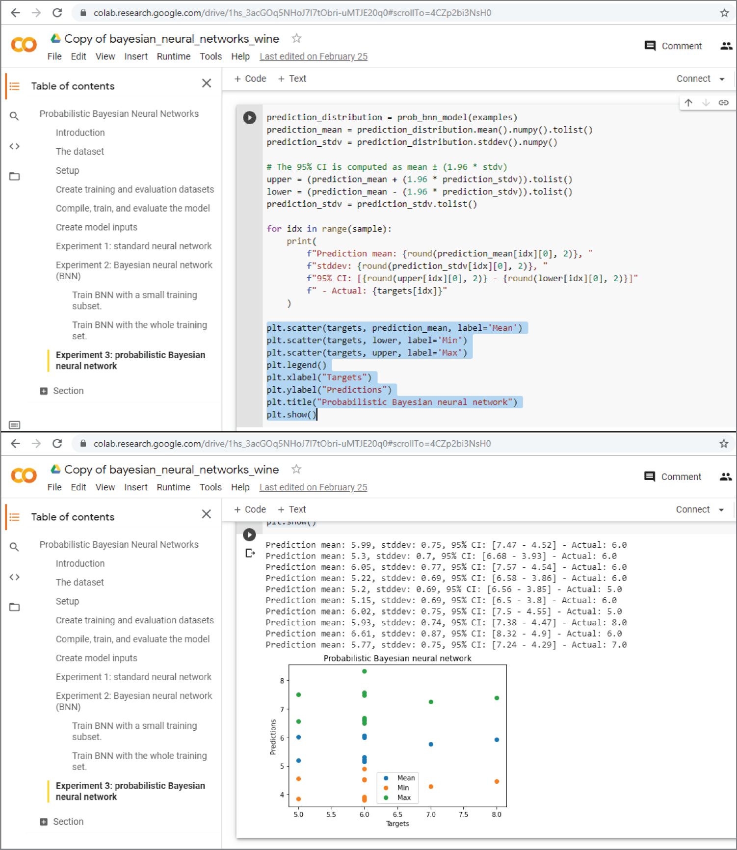
Figure 4.41: The code for plotting the mean, the maximum, and the minimum of the predictions (top), and the corresponding plot (bottom)
(Source: https://colab.research.google.com/drive/1hs_3acGOq5NHoJ7l7tObri-uMTJE20q0#scrollTo=13ypK49LNsHo)
4.8 Meta Learning
Meta learning is another approach in AI that has become popular in recent years. Meta is a Greek word meaning “after” or “beyond.” When used as a prefix, meta means “about.” So, meta learning is “learning about learning” or “learn to learn.”
The term meta learning was coined by Donald Maudsley in 1979, where he described a mechanism by which people are becoming “increasingly in charge of the patterns of perception, inquiry, learning, and development that they have internalized.” Later in 1985, John Biggs used the concept of meta learning to describe the state of “being conscious of one's learning and taking control of it.” You can describe meta learning as an awareness and understanding of the process of learning itself, like thinking about thinking.
Meta learning in AI is essentially about using high-level or meta-level AI to optimize lower-level AI, so that it can learn to learn effectively and quickly, as illustrated in Figure 4.42.
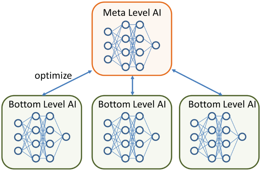
Figure 4.42: The schematic architecture of meta learning
The following are two interesting articles that give a comprehensive introduction to the meta learning, including all the mathematics behind it:
https://jameskle.com/writes/meta-learning-is-all-you-need
https://lilianweng.github.io/lil-log/2018/11/30/meta-learning.html
The following two GitHub sites give a curated list of meta learning papers, codes, books, blogs, videos, datasets, and other resources.
https://github.com/sudharsan13296/Awesome-Meta-Learning
https://github.com/dragen1860/awesome-meta-learning
The following GitHub site gives all the code examples for the book:
https://github.com/sudharsan13296/Hands-On-Meta-Learning-With-Python
The following two GitHub sites are meta learning projects implemented by PyTorch.
https://github.com/learnables/learn2learn
https://github.com/yaoyao-liu/meta-transfer-learning
https://github.com/facebookresearch/LearningToLearn/tree/main/ml3
4.9 Summary
This chapter gave a comprehensive overview of deep learning. Deep learning is the most important aspect of AI and a subset of machine learning. Deep learning is the hottest research topic in AI.
Deep learning neural networks are built on traditional neural networks, which are also called artificial neural networks. Deep learning neural networks can be generally divided into two types: convolutional neural networks and recurrent neural networks. Convolutional neural networks are the most popular deep learning neural networks, which include networks such as LeNet, AlexNet, GoogLeNet (Inception), VGG, ResNet, DenseNet, MobileNet, YOLO, and so on.
Apart from traditional convolutional neural networks, there are also new types of networks, such as U-Net, AutoEncoder, siamese neural networks, and capsule networks.
Recurrent neural networks are another popular deep learning neural network. Convolutional neural networks are specialized in processing images, while recurrent neural networks are specialized in processing sequences.
Transformers are new deep learning neural networks that are mainly used in the field of natural language processing. Transformers are gradually making recurrent neural networks obsolete.
Graph neural networks are a special type of recurrent neural network that can take graphs as input data.
Bayesian neural networks are neural networks whose weights or parameters are expressed as a distribution rather than a deterministic value. The learning of Bayesian neural networks is done by Bayesian inference.
4.10 Chapter Review Questions
| Q4.1. | What is the difference between machine learning and deep learning? |
| Q4.2. | What is an artificial neural network? |
| Q4.3. | What is a convolutional neural network? |
| Q4.4. | Explain the terms of convolutional layer, pooling layer, activation layer, dropout layer, and fully connected layer, in the context of convolutional neural networks. |
| Q4.5. | Compare the features of three commonly used activation functions: REctified Linear Unit (ReLU), hyperbolic tangent, and the sigmoid function. |
| Q4.6. | Use a table to compare the characteristic features of AlexNet, Inception, VGG, ResNet, DenseNet, MobileNet, and EffecientNet. |
| Q4.7. | What is U-Net, and what is it best used for? |
| Q4.8. | What is AutoEncoder? |
| Q4.9. | What is a Siamese neural network? Draw a schematic diagram of a Siamese neural network. |
| Q4.10. | What are differences between zero-shot learning, one-shot learning, few-shot learning, and n-shot learning? |
| Q4.11. | What is a capsule network, and how does it differ from a convolutional neural network? |
| Q4.12. | What is a recurrent neural network? |
| Q4.13. | What is a long-short term memory (LSTM) network? |
| Q4.14. | What is a transformer? |
| Q4.15. | What is BERT and ALBERT? |
| Q4.16. | What is GPT-3? |
| Q4.17. | What is a graph neural network? |
| Q4.18. | What is a Bayesian neural network? |