
Have you ever thought of colorizing the old B&W photograph of your granny? You would probably approach a Photoshop artist to do this job for you, paying them hefty fees and awaiting a couple of days/weeks for them to finish the job. If I tell you that you could do this with a deep neural network, would you not get excited about learning how to do it? Well, this chapter teaches you the technique of converting your B&W images to a colorized image almost instantaneously. The technique is simple and uses a network architecture known as AutoEncoders. So, let us first look at AutoEncoders.
AutoEncoders
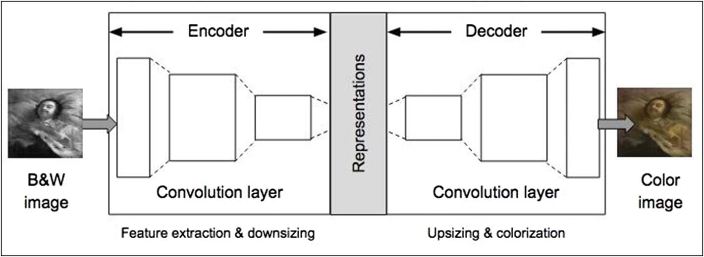
AutoEncoder architecture
On the left, we have a B&W image fed to our network. On the right, where we have the network output, we have a colorized image of the same input content. What goes in between can be described like this. The Encoder processes the image through a series of Convolutional layers and downsizes the image to learn the reduced dimensional representation of the input image. The decoder then attempts to regenerate the image by passing it through another series of Convolutional layers, upsizing and adding colors in the process.
Now, to understand how to colorize an image, you must first understand the color spaces.
Color Spaces
A color image consists of the colors in a given color space and the luminous intensity. A range of colors are created by using the primary colors such as red, green, blue. This entire range of colors is then called a color space, for example, RGB. In mathematical terms, a color space is an abstract mathematical model that simply describes the range of colors as tuples of numbers. Each color is represented by a single dot.
RGB
YCbCr
Lab
RGB is the most commonly used color space. It contains three channels – red (R), green (G), and blue (B). Each channel is represented by 8 bits and can take a maximum value of 256. Combined together, they can represent over 16 million colors.
The JPEG and MPEG formats use the YCbCr color space. It is more efficient for digital transmission and storage as compared to RGB. The Y channel represents the luminosity of a grayscale image. The Cb and Cr represent the blue and red difference chroma components. The Y channel takes values from 16 through 235. The Cb and Cr values range from 16 to 240. Be careful, the combined value of all these channels may not represent a valid color. In our application of colorization, we don't use this color space.
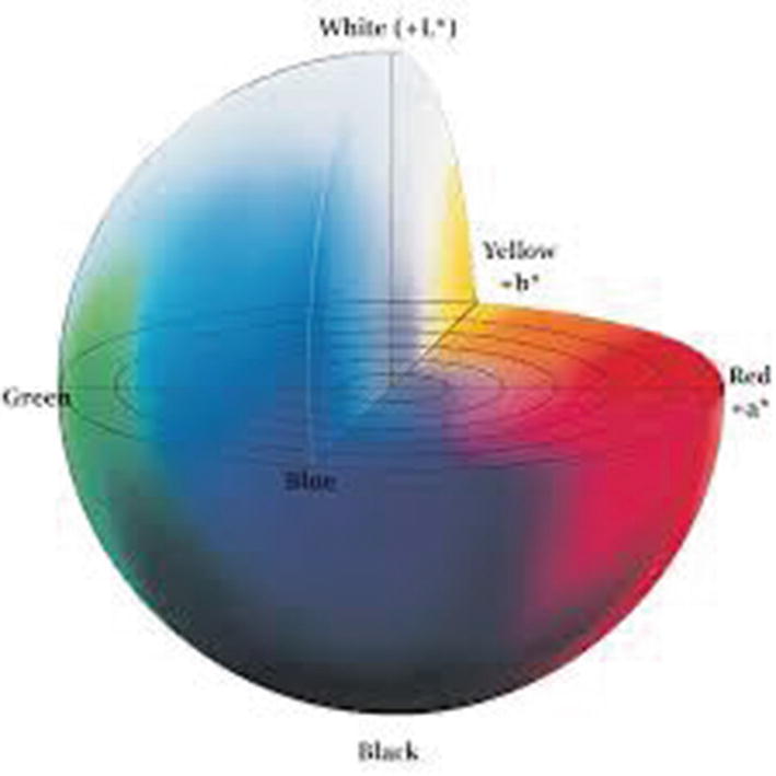
The Lab color space
The Lab color space is larger than the gamut of computer displays and printers. Then, a bitmap image represented as a Lab requires more data per pixel to obtain the same precision as an RGB or CMYK. Thus, the Lab color space is typically used as an intermediary rather than an end color space.
The L channel represents the luminosity and takes values in the range 0 to 100. The “a” channel codes from green (-) to red (+), and the “b” channel codes from blue (-) to yellow (+). For an 8-bit implementation, both take values in the range -127 to +127. The Lab color space approximates the human vision. The amount of numerical change in these component values corresponds to roughly the same amount of visually perceived change.
We use the Lab color space in our project. By separating the grayscale component which represents the luminosity, the network has to learn only two remaining channels for colorization. This helps in reducing the network size and results in faster convergence.
I will now discuss the different network topologies for our AutoEncoders.
Network Configurations
Vanilla
Merged
Merged model using pre-trained network
I will now discuss all three models.
Vanilla Model
The vanilla model has the configuration shown in Figure 14-1, where the Encoder has a series of Convolutional layers with strides for downsizing the image and extracting features. The Decoder too has Convolutional layers which are used for upsizing and colorization. In such autoencoders, the encoders are not deep enough to extract the global features of an image. The global features help us in determining how to colorize certain regions of the image. If we make the encoder network deep, the dimensions of the representation would be too small for the decoder to faithfully reproduce the original image. Thus, we need two paths in an Encoder – one to obtain the global features and the other one to obtain a rich representation of the image. This is what is done in the next two models. You will be constructing a vanilla network for the first project in this chapter .
Merged Model
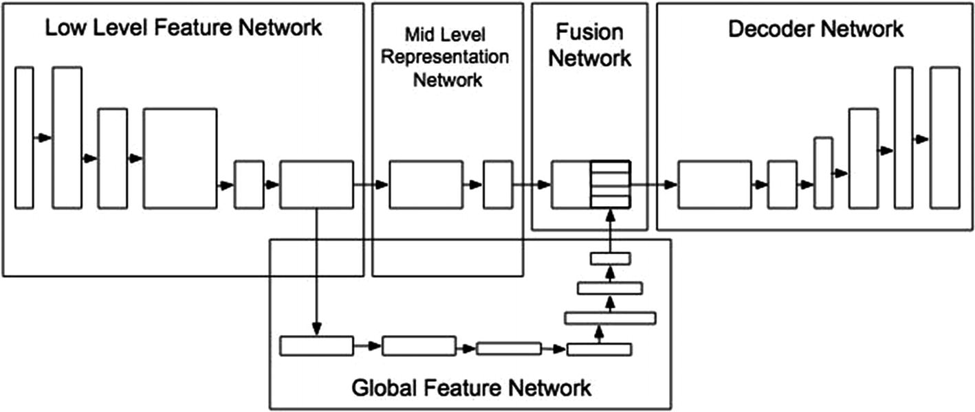
Merged model architecture
An eight-layer Encoder was used to extract the mid-level representations. The output of the sixth layer is forked and fed through another seven-layer network to extract the global features. Another Fusion network then concatenates the two outputs and feeds them to the decoder.
Merged Model Using Pre-trained Network
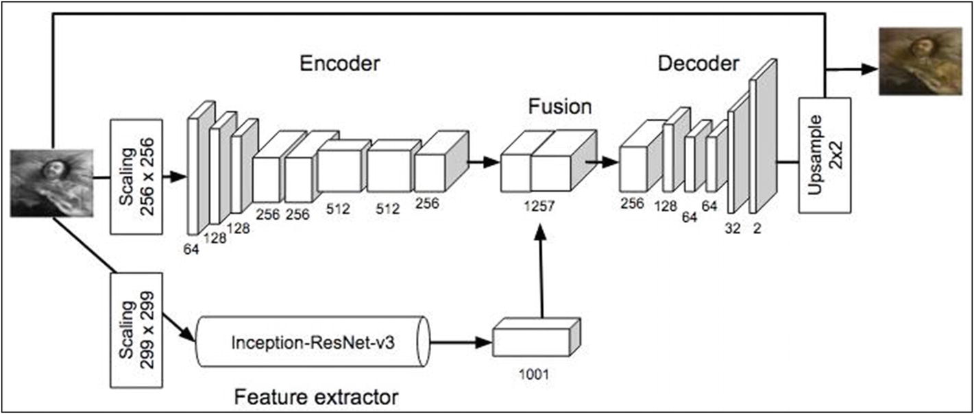
Model using a pre-trained network
The feature extraction is done by a pre-trained ResNet.
In the second project in this chapter, I will show you how to use a pre-trained model for feature extraction, though you will not be constructing as complicated a model as shown in this schematic.
With this introduction to AutoEncoders and their configurations, let us start with some practical implementations of them.
AutoEncoder
In this project, you will be using the vanilla autoencoder.
Loading Data
The os.walk gets all the filenames present in the folder.
When you run this code, you will discover that there are 86 bad images in the set.
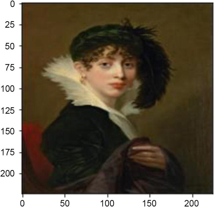
A sample image
Creating Training/Testing Datasets
The train_test_split method as specified in the test_size parameter reserves 20 images for testing.
Preparing Training Dataset
For training the model, we will convert the images from RGB to Lab format. As said earlier, the L channel is the grayscale. It represents the luminance of the image. The “a” is the color balance between green and red, and the “b” is the color balance between blue and yellow.
If each image is skewed, the model will learn better. The shear_range tilts the image to the left or right, and the other parameters zoom, rotation, and horizontal flip have their respective meanings.
The function first converts the given image from RGB to grayscale by calling the rgb2gray method. The image is then converted to Lab format by calling the rgb2lab method. If we take Lab color space, we need to predict only two components as compared to other color spaces where we would need to predict three or four components. As said earlier, this helps in reducing the network size and results in a faster convergence. Finally, we extract the L, a, and b components from the image.
Defining Model
Both the Encoder and Decoder contain few Conv2D layers. The Encoder through a series of layers downsamples the image to extract its features, and the Decoder through its own set of layers attempts to regenerate the original image using upsampling at various points and adding colors to the grayscale image to create a final image of size 256x256. The last decoder layer uses tanh activation for squashing the values between –1 and +1. Remember that we had earlier normalized the a and b values in the range –1 through +1.
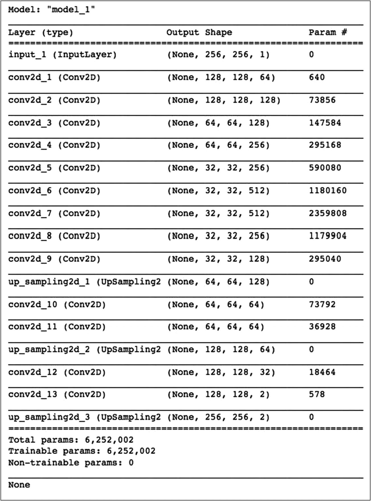
Autoencoder model summary

Model plot
Model Training
It took me slightly over a minute per epoch to train the model on a GPU. By using the pre-trained model, this training time came down to about a second per epoch as you would see when you run the second project in this chapter.
Testing
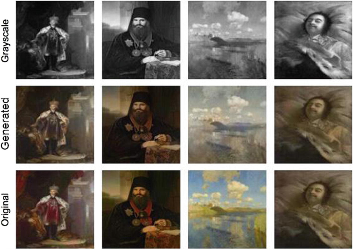
Model inference
The first row is the set of grayscale images created from the original color images given in the third row. The middle row shows the images generated by the model. As you can see, the model is able to generate the images close enough to the original images.
Now, I will show you how to use this model on an unseen image of a different size.
Inference on an Unseen Image
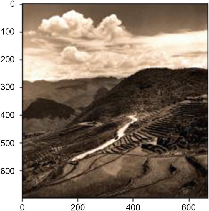
Sample image with different dimensions

A colorized image generated by the custom autoencoder model
Full Source
AutoEncoder_Custom
Now, I will show you how to use a pre-trained model for features extraction, thereby saving you a lot of training time and giving better feature extraction.
Pre-trained Model as Encoder
There are several pre-trained models available for image processing. You have used one such VGG16 model in Chapter 12. The use of this model allows you to extract the image features, and that is what we did in our previous program by creating our own encoder. So why not use the transfer learning by using a VGG16 pre-trained model in place of an encoder? And that is what I am going to demonstrate in this application. The use of a pre-trained model would certainly provide better results as compared to your own defined encoder and a faster training too.
Project Description
You will be using the same image dataset as in the previous project. Thus, the data loading and preprocessing code would remain the same. What changes is the model definition and the inference. So, I will describe only the relevant changes. The entire project source is available in the book’s download site and also given at the end of this section for your quick reference. The project is named AutoEncoder-TransferLearning.
Defining Model
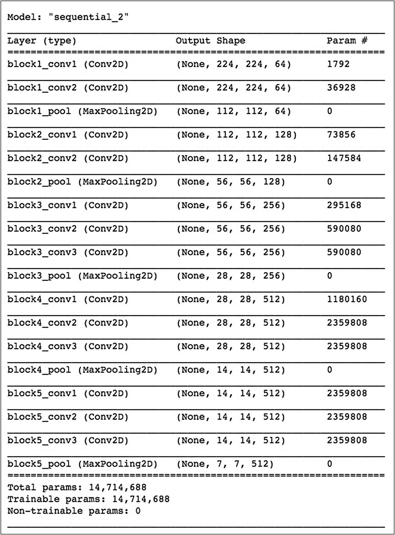
Pre-trained encoder model summary
Extracting Features
Defining Network
For the encoder, we just specify the input, and the decoder architecture is the same as in the previous example where we keep on upsizing the image and adding colors to it.
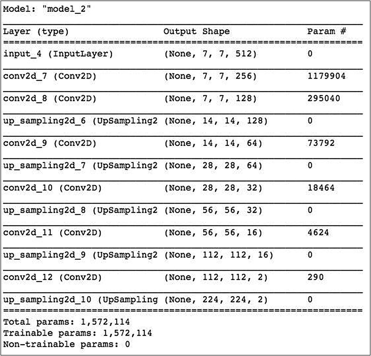
Encoder decoder model summary
Model Training
We use the Adam optimizer and the mse loss for training. Training the network on a GPU, the epoch time was about a second – a considerable improvement over our earlier network. As we have used a pre-trained encoder, only the decoder parameters need to be trained.
Inference
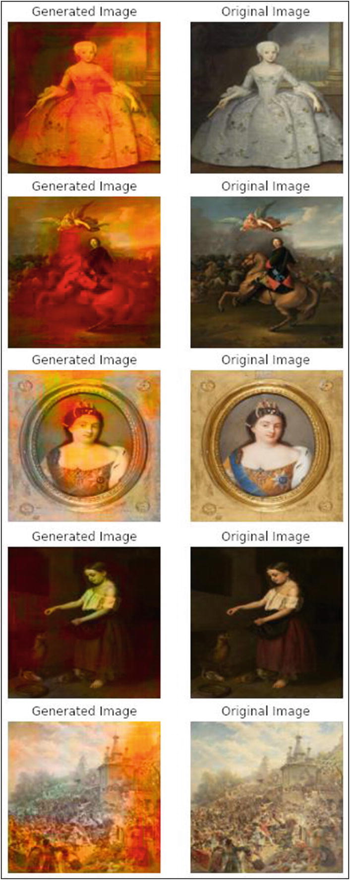
Model inference on test images
Inference on an Unseen Image
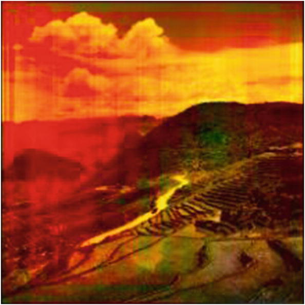
A colorized image generated by the autoencoder transfer learning model
Full Source
AutoEncoder_TransferLearning
Summary
The use of deep neural networks makes it possible to add colors to a B&W image. You learned to create AutoEncoders, which we used for colorizing B&W images. The AutoEncoder contains an Encoder to extract the image features, and the Decoder recreates the image using the representations extracted from the encoder. You also learned how to use a pre-trained image classifier to extract the image features for using it as a part of the Encoder.