
Did you ever imagine that neural networks could be used for generating complex color images? How about Anime? How about the faces of celebrities? How about a bedroom? Doesn’t it sound interesting? All these are possible with the most interesting idea in neural networks and that is Generative Adversarial Networks (GANs). The idea was introduced and developed by Ian J. Goodfellow in 2014. The images created by GAN look so real that it becomes practically impossible to differentiate between a fake and a real image. Be warned, to generate complex images of this nature, you would require lots of resources to train the network, but it does certainly work as you would see when you study this chapter. So let us look at what is GAN.
GAN – Generative Adversarial Network
In GAN, there are two neural network models which are trained simultaneously by an adversarial process. One network is called a generator, and the other is called a discriminator. A generator (an artist) learns to create images that look real. A discriminator (the critic) learns to tell real images apart from the fakes. So these are two competing models which try to beat each other. At the end, if you are able to train the generator to outperform the discriminator, you would have achieved your goal.
How Does GAN Work?
- 1.
Keeping the generator idle, train the discriminator. Train the discriminator on real images for a number of epochs and see if it can correctly predict them as real. In the same training phase, train the discriminator on the fake images (generated by the generator) and see if it can predict them as fake.
- 2.
Keeping the discriminator idle, train the generator. Use the prediction results made by the discriminator on the fake images to improve upon those images.
The preceding steps are repeated for a large number of epochs, and the results (fake images) are examined manually to see if they look real. If they do, stop the training. If not, continue the preceding two steps until the fake image looks real.
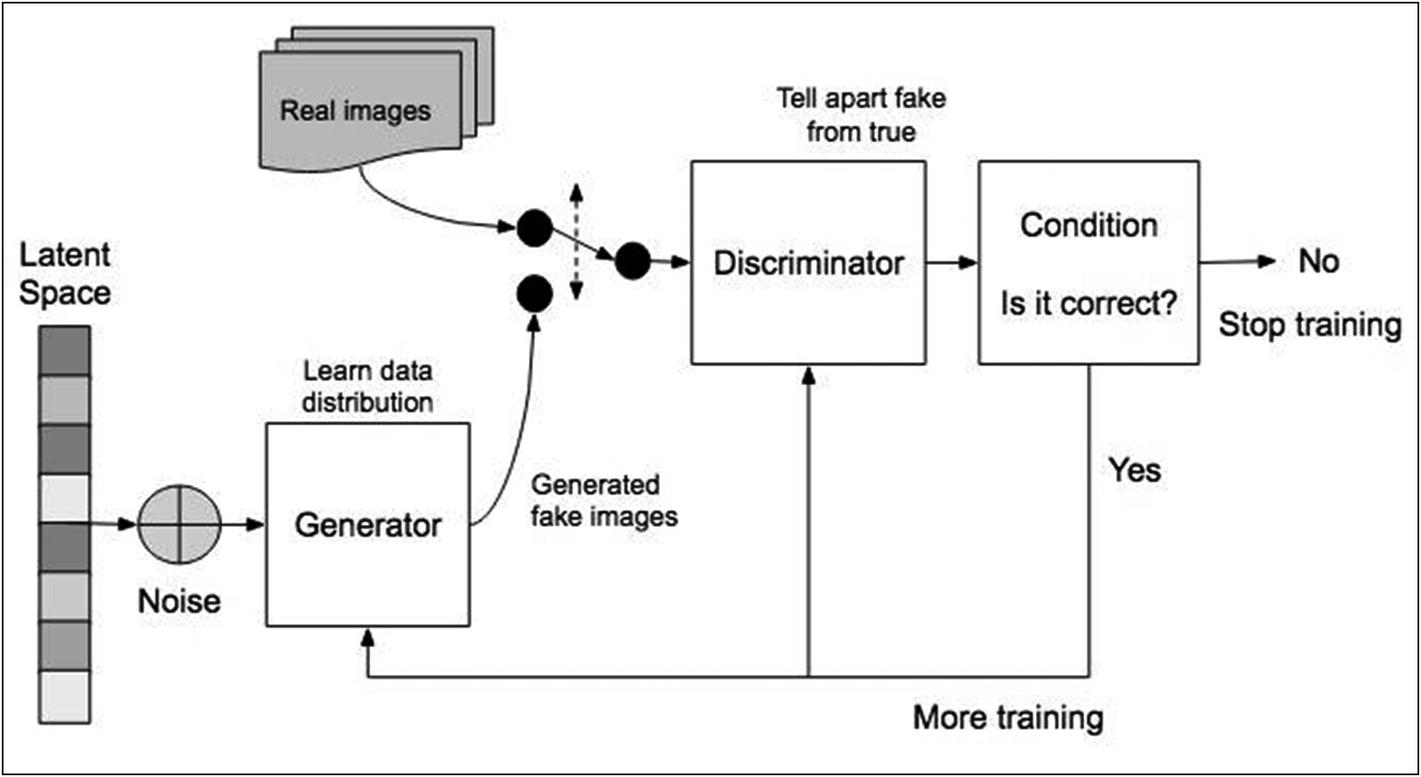
GAN working schematic
The Generator
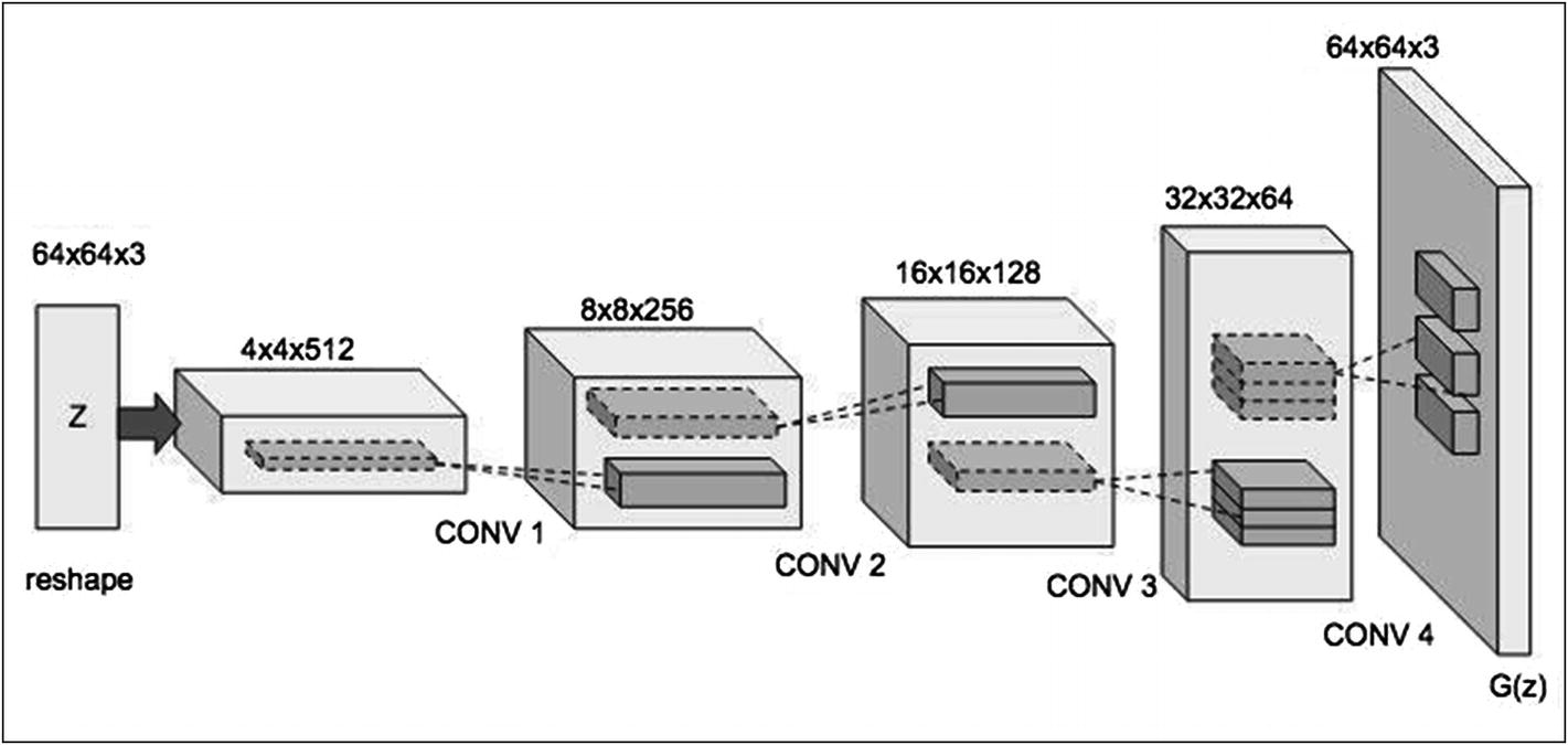
Generator architecture
The generator takes a random noise vector of some dimension. We will be using a dimension of 100 in our examples. From this random vector, it generates an image of 64x64x3. The image is upscaled by a series of transitions through convolutional layers. Each convolutional transpose layer is followed by a batch normalization and a leaky ReLU. The leaky ReLU has neither vanishing gradient problems nor dying ReLU problems. The leaky ReLU attempts to fix the “dying ReLU” problem. The ReLU will acquire a small value of 0.01 or so instead of dying out to 0. We use strides in each convolutional layer to avoid unstable training.
Note how, at each convolution, the image is upscaled to create a final image of 64x64x3.
The Discriminator
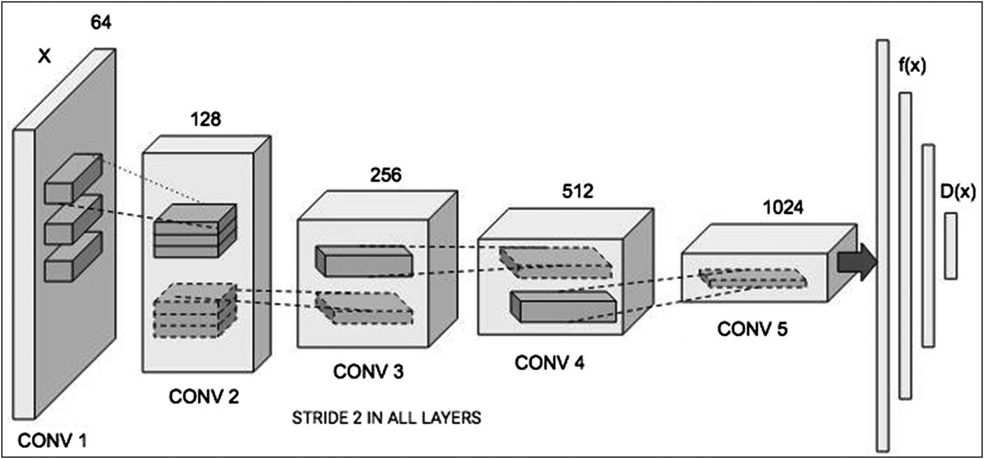
Discriminator architecture
The discriminator too uses Convolutional layers and downsizes the given image for evaluation.
Mathematical Formulation
![$$ frac{mathit{min}}{G}frac{mathit{max}}{D}Vleft(D,G
ight)=frac{mathit{min}}{G}frac{mathit{max}}{D}left({E}_{zsim {P}_{data}(x)}left[ logD(x)
ight]+{E}_{zsim {P}_z(z)}left[mathit{log}left(1-Dleft(G(z)
ight)
ight)
ight]
ight) $$](https://imgdetail.ebookreading.net/20201209/5/9781484261507/9781484261507__artificial-neural-networks__9781484261507__images__495303_1_En_13_Chapter__495303_1_En_13_Chapter_TeX_Equa.png)
where G represents the generator and D the discriminator. The data(x) represents the distribution of real data and pz(z) the distribution of generated or fake data. The x represents a sample from real data and z from the generated data. The D(x) represents the discriminator network and G(z) the generator network.

The discriminator loss while training on the fake data coming from the generator is expressed as

For real data, the discriminator prediction should be close to 1. Thus, the equation 1 should be maximized in order to get D(x) close to 1. The first equation is the discriminator loss on real data, which should be maximized in order to get D(G(z)) close to 1. Because the second equation is the discriminator loss on the fake data, it should also be maximized. Note that the log is an increasing function.
For the second equation, the discriminator prediction on the generated fake data should be close to zero. In order to maximize the second equation, we have to minimize the value of D(G(z)) to zero. Thus, we need to maximize both losses for the discriminator. The total loss of the discriminator is the addition of two losses given by equations 1 and 2. Thus, the combined total loss will also be maximized.
![$$ {L}^{(G)}=mathit{min}left[mathit{log}left(D(x)
ight)+mathit{log}left(1-Dleft(G(z)
ight)
ight)
ight] $$](https://imgdetail.ebookreading.net/20201209/5/9781484261507/9781484261507__artificial-neural-networks__9781484261507__images__495303_1_En_13_Chapter__495303_1_En_13_Chapter_TeX_Equ3.png)
We need to minimize this loss during the generator training.
Digit Generation
In this project, we will use the popular MNIST dataset provided by Kaggle. As you know, the dataset consists of images of handwritten digits. We will create a GAN model to create additional images looking identical to these images. Maybe this could be helpful to somebody in increasing the training dataset size in their future developments.
Creating Project
Loading Dataset
The shape is (5949, 28, 28). Thus, we have 5949 images of size 28x28. It is a huge repository. Our model will try to produce images of this size, matching the looks of these images.

Sample images
We will now prepare the dataset for training.
Preparing Dataset
As each color value in the image is in the range of 0 through 256, we normalize these values to the scale of –1 to 1 for better learning. The mean value is 127.5, and thus the following equation will normalize the values in the range –1 to +1. You could have alternatively chosen 255 to normalize the values between 0 and 1.
Next comes the important part of our application, and that is defining the model for our generator.
Defining Generator Model
The generator’s purpose is to create images containing digit 9 which look similar to the images in our training dataset.
The input to this layer is specified as 100 because later on we will use a noise vector of dimension 100 as an input to this GAN model. We will start with an image size of 7x7 and keep upscaling it to a final destination size of 28x28. The z-dimension 256 specifies the filters used for our image, which eventually gets converted to 3 for our final image.
We add the activation layer as a leaky ReLU.
The first parameter is the dimensionality of the output space, that is, the number of output filters in the convolution. The second parameter is the kernel_size that actually specifies the height and width of the convolution filter. The third parameter specifies the strides of the convolution along the height and width. To understand strides, consider a filter being moved across the image from left to right and top to bottom, 1 pixel at a time. This movement is referred to as the stride. With a stride of (2, 2), the filter is moved 2 pixels on each side, upscaling the image by 2x2.
The output image will now be of size 14x14.
The last layer uses tanh activation and the map parameter value of 1, thus giving us a single output image.
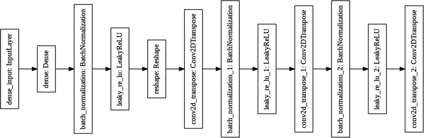
Generator architecture

Generator model summary
Testing Generator
Random image generated by the generator
The output indicates that the image has dimensions of 28x28, as desired by us.
Next , we will define the discriminator.
Defining Discriminator Model
The discriminator uses just two convolutional layers. The output of the last convolutional layer is of type (batch size, height, width, filters). The Flatten layer in our network flattens this output to feed it to our last Dense layer in the network.
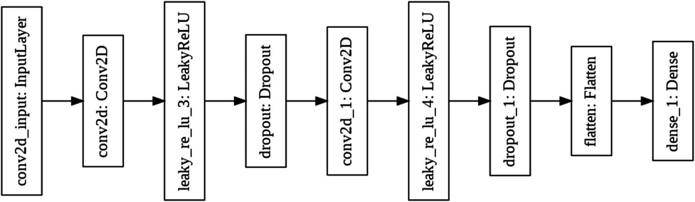
Discriminator architecture
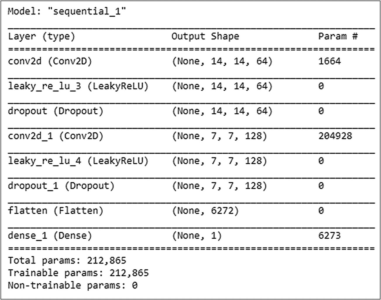
Discriminator model summary
Note that the discriminator has only around 200,000 trainable parameters.
Testing Discriminator
The decision value is 0.0033, a positive integer indicating that the image is real. A maximum value of 1 tells us that the model is sure about the image being real. If you generate another image using our generator and test the output of the discriminator, you may get a negative result. This is because we have not yet trained our generator and discriminator on some datasets.
Defining Loss Functions
We use Keras’s binary cross-entropy function for our purpose. Note that we have two classes – one (1) for a real image and the other (0) for a fake one. We compute our loss for both these classes, and thus it makes our problem a binary classification problem. Thus, we use a binary cross-entropy for the loss function.
The return value of the function is the quantification of how well the generator is able to trick the discriminator. If the generator does its job well, the discriminator will classify the fake image as real, returning a decision of 1. Thus, the function compares the discriminator’s decision on the generated image with an array of ones.
We first let the discriminator consider that the given image is real and then compute the loss with respect to an array of ones. We then let the discriminator consider that the image is fake and then ask it to calculate the loss with respect to an array of zeros. The total loss as determined by the discriminator is the sum of these two losses.
You will now write a few utility functions, which are used during training.
Defining Few Functions for Training
We will train the model for 100 epochs. You can always change this variable to your choice. A higher number of epochs would generate a better image for the digit 9, which we are trying to generate. The noise dimension is set to 100 which is used while creating the random image for our first input to the generator network. The seed is set to random data for one image.
Checkpoint Setup
In case of disconnection, you can continue the training from the last checkpoint. I will show you how to do this.
Setting Up Drive
The checkpoint data is saved to a folder called GAN1/Checkpoint in your Google Drive. So, before running the code, make sure that you have created this folder structure in your Google Drive.
Next, we write a gradient_tuning function.
Model Training Step
Both our generator and discriminator models will be trained in several steps. We will write a function for these steps.
We will use the gradient tape (tf.GradientTape) for automatic differentiation on both the generator and discriminator. The automatic differentiation computes the gradient of a computation with respect to its input variables. The operations executed in the context of a gradient tape are recorded onto a tape. The reverse mode differentiation is then used to compute the new gradients. You need not get concerned with these operations for understanding how the models are trained.
Gradient tuning function
The function uses a global epoch_number to track the epochs, in case of disconnection and continuing thereof. The test_input to the model will always be our random seed. The inference is done on this seed after setting training to False for batch normalization to be effective. We then display the image on the user’s console and also save it to the drive with epoch_number added as a suffix.
Using these functions, you will now write code to train the models and generate some output.
Model Training
Model training function
Images for digit 9 generated by the program
|
As you can see from the output, the network is able to create an acceptable output just after 20/30 epochs, and at 70 and above, the quality is best.
In my run of this application, it took approximately 10 seconds for each epoch on a GPU. Many times, for more complex image generation, it may take several hours to get an acceptable output. In such cases, checkpoints would be useful in restarting the training.
Full Source
DigitGen-GAN.ipynb
In this example, you trained a model to generate the handwritten digits. In the next example, I will show you how to create handwritten characters.
Alphabet Generation
Just the way Kaggle provides the dataset for digits, the dataset for handwritten alphabets is available in another package called extra-keras-datasets. You will be using this dataset to generate the handwritten alphabets. The generator and discriminator models, their training, and inference all remain the same as in the case of digit generation. So, I am just going to give you the code of how to load the alphabets dataset from the Kaggle site and will give you the output of generated images. The full project source is available in the book’s repository under the name emnist-GAN.
Downloading Data
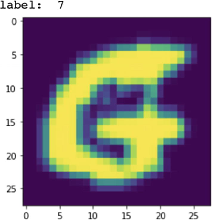
Image for the handwritten G character
Like in the digits database, each image has a dimension of 28x28. Thus, we will be able to use our previous generator model that produces images of this dimension. One good thing for our experimentation here is that each alphabet label takes the value of its position in the alphabets set. For example, the letter a has a label value of 1, the letter b has a label value of 2, and so on.
Creating Dataset for a Single Alphabet

Sample handwritten character images
Okay, now your dataset is ready. The rest of the code for preprocessing the data, defining models, loss functions, optimizers, training, and so on remains the same as the digit generation application. I will not reproduce the code here, I will simply show you the final output of my run.
Program Output
Images generated at various epochs
|

As in the case of digit generation, you can notice that the model gets quickly trained during the first few epochs, and by the end of 100 epochs, you have a quality output.
Full Source
emnist-GAN.ipynb
Printed to Handwritten Text
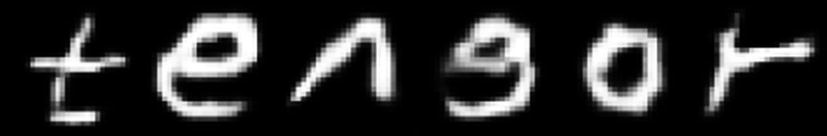
Sample text created by combining images
Next comes the creation of a more complex image.
Color Cartoons
So far, you have created images of handwritten digits and alphabets. What about creating complex color images like cartoons? The techniques that you have learned so far can be applied to create complex color images. And that is what I am going to demonstrate in this project.
Downloading Data
Creating Dataset
Displaying Images

Sample anime images
There are 30,000 RGB images, each of size 64x64. At this point, you are ready for defining your models, training them, and doing inference. The rest of the code that follows here is exactly identical to the earlier two projects, and thus I am not reproducing the code here. You may look up the entire source code in the project download. I will present only the output at different epochs.
Output
Sample images generated at various epochs
|
You can see that by about 1000 epochs, the network learns quite a bit to reproduce the original cartoon image. To train the model to generate a real-like image, you would need to run the code for 10,000 epochs or more. Each epoch took me about 16 seconds to run on a GPU. Basically, what I wanted to show you here is that the GAN technique that we develop for creating trivial handwritten digits can be applied as is to generate complex large images too.
Full source
CS-Anime.ipynb
Summary
The Generative Adversarial Network (GAN) provides a novel idea of mimicking any given image. The GAN consists of two networks – generator and discriminator. Both models are trained simultaneously by an adversarial process. In this chapter, you studied to construct a GAN network, which was used for creating handwritten digits, alphabets, and even animes. To train a GAN requires huge processing resources. Yet, it produces very satisfactory results. Today, GANs have been successfully used in many applications. For example, GANs are used for creating large image datasets like the handwritten digits provided on the Kaggle site that you used in the first example in this chapter. It is successful in creating human faces of celebrities. It can be used for generating cartoon characters like the anime example in this chapter. It has also been applied in the areas of image-to-image and text-to-image translations. It can be used for creating emojis from photos. It can also be used for aging faces in the photos. The possibilities are endless; you should explore further to see for yourself how people have used GANs in creating many interesting applications. With the techniques that you have learned in this chapter, you would be able to implement your own ideas to add this repository of endless GAN applications.