
Introduction
Any machine learning project consists of many stages that include training, evaluation, prediction, and finally exporting it for serving on a production server. You learned these stages in previous chapters where the classification and regression machine learning projects were discussed. To develop the best performing model, you played around with different ANN architectures. Basically, you experimented with several different prototypes to achieve the desired results. Prior to TF 2.0, this entire experimentation was not so easy as for every change that you make in the code, you were required to build a computational graph and run it in a session. The estimators that you are going to study in this chapter were designed to handle all this plumbing. The entire process of creating graphs and running them in sessions was a time-consuming job and posed lots of challenges in debugging the code.
Additionally, after the model is fully developed, there was a challenge of deploying it to a production environment where you may wish to deploy it in a distributed environment for better performance. Also, you may like to run the model on a CPU, GPU, or a TPU. This necessitated code changes. To help you with all these issues and to bring everything under one umbrella, estimators were introduced, albeit prior to TF 2.0. However, the estimators, which you are going to learn in this chapter and will be using in all your future projects, are capable of taking advantage of the many new facilities introduced in TF 2.x. For example, there is a clear separation between building a data pipeline and the model development. The deployment on a distributed environment too occurs without any code change. The enhanced logging and tracing make debugging easier. In this chapter, you will learn how estimator achieves this.
What is an estimator?
What are premade estimators?
Using a premade estimator for classification problems
Using a premade estimator for regression problems
Building custom estimators on Keras models
Building custom estimators on tfhub modules
Estimator Overview
A TensorFlow estimator is a high-level API that unifies several stages of machine learning development under a single umbrella. It encapsulates the various APIs for training, evaluation, prediction, and exporting your model for production use. It is a high-level API that provides a further abstraction to the existing TensorFlow API stack.
API Stack
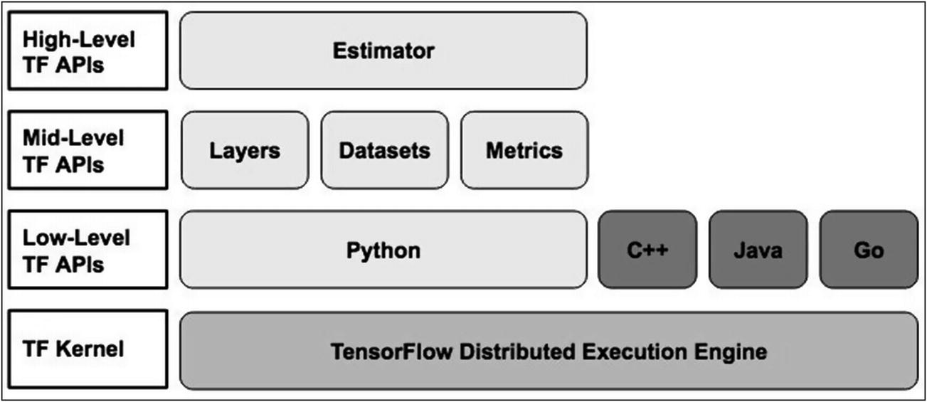
TensorFlow API stack
So far, you have mostly used mid-level APIs; the use of low-level APIs becomes a rare necessity when you need a finer control over the model development. Now, after learning the estimator API, you may not even use the mid-level APIs for your model developments. But then what happens to the models which you have already developed – can they benefit from using this API? And if so, how to make them use this API? Fortunately, the TensorFlow team has developed an interface that allows you to migrate the existing models to use the estimator interface. Not only that, they have created a few estimators on their own to get you quickly started. These are called premade estimators. They are not just the start-up points. They are fully developed and tested for you to use in your immediate projects. If at all these do not meet your purpose or if you want to migrate existing models to facilitate the benefits offered by the estimator, you can develop custom estimators using the estimator API. Before you learn how to use premade estimators and to build your own ones, let me discuss its benefits in more detail.
Estimator Benefits
Providing a unified interface for train/evaluate/predict
Handling data input through an Input function
Creating checkpoints
Creating summary logs
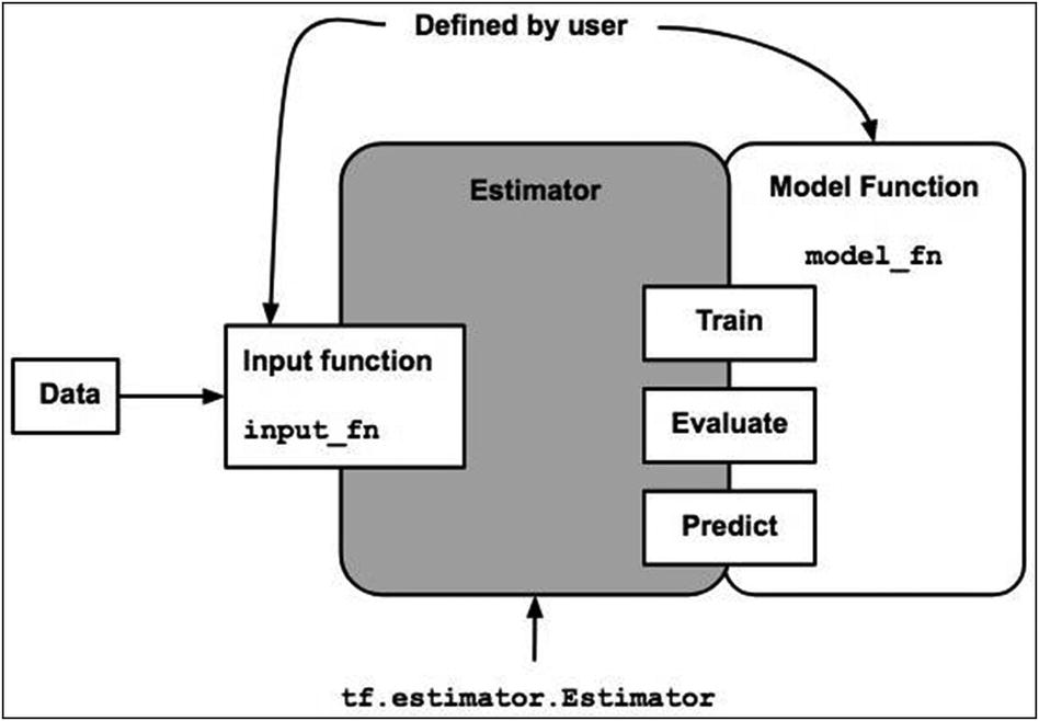
Estimator interface
As you can see in Figure 6-2, the estimator class provides three interface methods for training, evaluation, and predictions. So, once you develop an estimator object, you will be able to call the train, evaluate, and predict methods on the same object. Note that you need to send different datasets for each. This is achieved with the help of an input function. I have explained the structure of this input function in more detail later in this section. It is sufficient to say at this point that the introduction of the Input function simplifies your experimentation with different datasets.
The checkpoints created during training allow you to roll back to a known state and continue the training from this checkpoint. This would save you lots of training time, especially when the errors occur toward the fag end of an epoch. This also makes the debugging quicker. After the training is over, the summary logs created during evaluation can be visualized on TensorBoard, giving you quick insights on how good the model is trained.
After the model is trained to your full satisfaction, next comes the task of deployment. Deploying a trained model on CPU/GPU/TPU, even mobiles and the Web, and a distributed environment previously required several code changes. If you use an estimator, you will deploy the trained model as is or at the most with minimal changes on any of these platforms.
Having said all these benefits, let us first look at the types of estimators.
Estimator Types
Premade estimators
Custom estimators

Estimator classifications
The premade estimators are like a model in a box where the model functionality is already written by the TensorFlow team. On the other hand, in custom estimators, you are supposed to provide this model functionality. In both cases, the estimator object that you create will have a common interface for training, evaluation, and prediction. Both can be exported for serving in a similar way.
The TensorFlow library provides a few premade estimators for your immediate go; if these do not meet your purpose and/or you want to migrate your existing models to get the benefits of estimators, you would create your own estimator class. All estimators are subclasses of the tf.estimator.Estimator base class.
The DNNClassifier, LinearClassifier, and LinearRegressor are the few examples of premade estimators. The DNNClassifier is useful for creating classification models based on dense neural networks, while the LinearRegressor is for handling linear regression problems. You will learn how to use both these classes in the upcoming sections in this chapter.
As part of building a custom estimator, you will be converting an existing Keras model to an estimator. Doing so will enable you to take advantage of the several benefits offered by estimators, which you have seen earlier. You will be building a custom estimator for the wine quality regression model that you developed in the previous chapter. Finally, I will also show you how to build a custom estimator based on tfhub modules.
To work with the estimators, you need to understand two new concepts – Input functions and Feature columns. The input function creates a data pipeline based on tf.data.dataset that feeds the data to the model in batches for both training and evaluation. You may also create a data pipeline for inference. I will show you how to do this in the DNNClassifier project. Feature columns specify how the data is to be interpreted by the estimator. Before I discuss these Input function and Feature column concepts, I will give you an overview of the development of an estimator-based project.
Workflow for Estimator-Based Projects
Loading data
Data preprocessing
Defining Features columns
Defining the Input function
Model instantiation
Model training
Model evaluation
Judging a model’s performance on TensorBoard
Using a model for predictions
As part of the learning that you have done in all previous chapters, you are definitely familiar with many steps in the preceding workflow. What needs attention is defining Features columns and the Input function. I will now describe these requirements.
Features Column

How Features columns are used
Fixed acidity (numeric)
Volatile acidity (numeric)
Citric acid (numeric)
…
Note we first obtain the vocabulary by calling the categorical_column_with_vocabulary_list method and then append the indicator columns to the list.
This list is passed as a parameter to the estimator constructor, as seen in Figure 6-4. If your model requires both numerical and categorical features, you will need to append both to your destination Features column.
The left block in Figure 6-4 shows data which is actually built by an Input function. This data will be input to the estimator’s train/evaluate/predict method calls.
Next, I will describe how to write the Input function.
Input Function
A dictionary of feature names (keys) and Tensors or Sparse Tensors (values) containing the corresponding feature data
A Tensor containing one or more labels
You may write separate functions based on this prototype for training/evaluation/inferencing.
I will now present you the practical implementation of the Input function taken from the example that is later discussed in this chapter. This would further clarify the concepts behind the Input function in your minds.

The Input function structure
The whole matter may look quite complicated; a practical example will help in clarifying the entire implementation, and that is what I am going to do next.
Premade Estimators
I will be discussing two types of premade estimators – one for classification and the other for a regression type of problems. First, I will describe a project for classification. We will use the premade DNNClassifier for this project. The DNNClassifier defines a deep neural network and classifies its input into several classes. You will be using the MNIST database for classifying the handwritten digits into ten numeric digits. The second project that I am going to describe uses the premade estimator called LinearRegressor. The project uses the Airbnb database for the Boston region. The database consists of several houses listed on Airbnb. For each listed house, several features are captured, and the price at which the house is sold/saleable is listed. Using this information, you will develop a regression model to predict the price at which a newly listed house would probably be sold.
The use of these two different models will give you a good insight into how to use the premade estimators on your own model development problems. So let us start with a classification model first.
DNNClassifier for Classification
We will use the MNIST database for this project. The dataset is available in the sklearn kit. It is the database of the handwritten digits. Our task is to use the premade classifier to recognize the digits embedded in these images. The output consists of ten classes, pertaining to the ten digits.
Loading Data
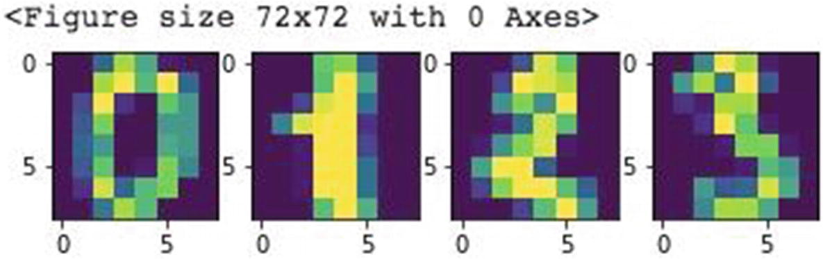
Sample images
Each image is of size 8 by 8 pixels.
Preparing Data
If you check the shape of data, you would notice that there are 1797 images, each consisting of totally 64 pixel values.
At this point, we are now ready to define our input function for the estimator.
Estimator Input Function
The first parameter defines the features data, the second defines the target values, and the third parameter specifies whether the data is to be used for training or evaluation. The data is processed in batches – the batch size is decided by the last parameter.
The data is converted into tensors by calling the from_tensor_slices method. The method takes an input consisting of the dictionary of features and the corresponding labels.
The shuffle method shuffles the dataset. We specify the buffer size of 1000 for shuffling. To handle datasets that are too large to fit in memory, the shuffling is done in batches of data. If the buffer size is greater than the number of data points in the dataset, you get a uniform shuffle. If it is 1, you get no shuffling at all.
Now comes the time to create an estimator instance.
Creating Estimator Instance
The constructor takes five parameters. The first parameter defines the network architecture. Here, we have defined three hidden layers in our architecture; the first layer contains 256 neurons, the second layer contains 128, and the third layer contains 64. The second parameter specifies the list of features that the data will have. Note that we have earlier created the feature_columns vector, so this is set as a default parameter. The third parameter specifies the optimizer to be used, set to Adagrad by default here. Adagrad is an algorithm for gradient-based optimization that does just this: It adapts the learning rate to the parameters, performing smaller updates. The n_classes parameter defines the number of output classes. In our case, it is 10, which is the number of digits 0 through 9. The last parameter model_dir specifies the directory name where the logs will be maintained.
Next comes the important part of model training.
Model Training
The method takes our input_fn as the parameter. The input_fn itself takes the features and labels data as the first two parameters. The training parameter is set to True so that the data will be shuffled. The number of steps is defined to be 2000. Let me explain what this means. In machine learning, an epoch means one pass over the entire training set. A step corresponds to one forward pass and back again. If you do not create batches in your dataset, a step would correspond to exactly one epoch. However, if you have split the dataset into batches, an epoch will contain many steps – note that a step is an iteration over a single batch of data. You can compute the total number of epochs executed during the full training cycle with the formula:
Number_of_epochs = (batch_size * number_of_steps) / (number_of_training_samples)
In our current example, the batch size is 32, the number of steps is 2000, and the number of training samples is 1707. Thus, it will take (32 * 2000) / 1707, that is, 38 epochs, to complete the training.
Model Evaluation
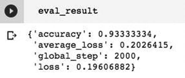
Model evaluation results
Sample evaluation metric
Next, you will learn how to predict an unseen data using our trained estimator.
Predicting Unseen Data
The input function uses the test data that we create for testing the two unseen data items.
Experimenting Different ANN Architectures

Evaluation results for more dense network
Evaluation metrics after adding dropout
Thus, you can easily experiment with several model architectures. You may also experiment with different datasets – for example, by changing the number of features included in the Features column list. Once satisfied with the model’s performance, you can save it to a file and then take the saved file straightaway to the production server for everybody’s use.
Project Source
DNNClassifier-Estimator full source
Now, as you have seen how to use a dense neural network classification estimator, I will show you how to use a premade classifier for regression problems.
LinearRegressor for Regression
As I mentioned in the previous chapter, neural networks can be used to solve regression problems. To support this claim, we also see a premade estimator in the TF libraries for supporting regression model development. I am going to discuss how to use this estimator in this section.
Project Description
The regression problem that we are trying to solve in this project is to determine the estimated selling price of a house in Boston. We will use the Airbnb dataset for Boston (www.kaggle.com/airbnb/boston) for this purpose. The dataset is multicolumnar and the various columns must be examined carefully for their suitableness as a feature in model development. Thus, for the regression model development, you would need to have a stringent preprocessing of data so that we sufficiently reduce the number of features and yet achieve a great amount of accuracy in predicting the house’s price.
Creating Project
Loading Data
The data is read into a pandas dataframe. You may check the data size by calling its shape method. You will know that there are 3585 rows and whopping 95 columns. Finding out a regression relationship between these 95 columns is not an easy task even for a highly skilled data analyst. That’s where once again you will realize that neural networks can come to your aid.
Out of the 95 columns that we have in the database, obviously not all will be of use to us in training our model. So, we need some data cleansing to remove the unwanted columns and standardize the remaining. We now do the data preprocessing as described further.
Features Selection
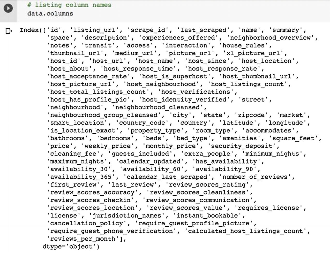
List of columns
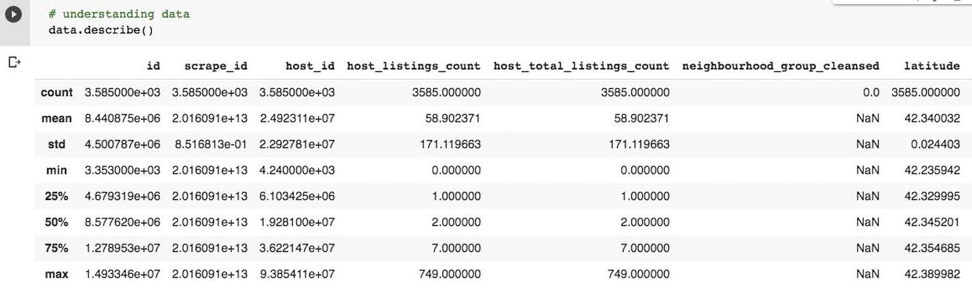
Data description
After selecting our features, we need to ensure that the data it contains is clean.
Data Cleansing
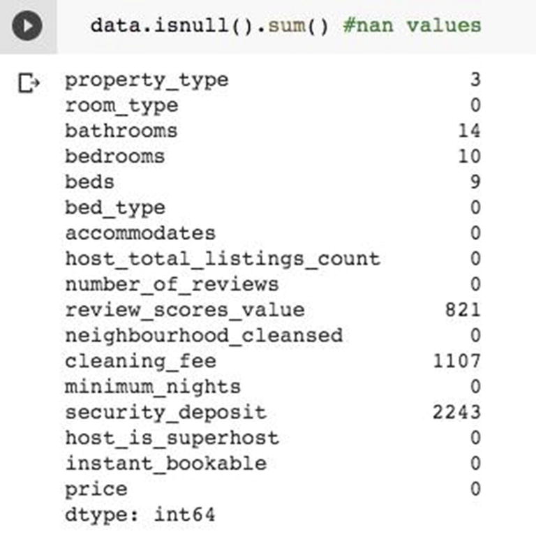
Checking null values

Examining data
In the loop, we also replace the null values with the field’s mean value.
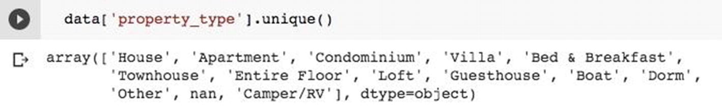
Unique values in categorical columns
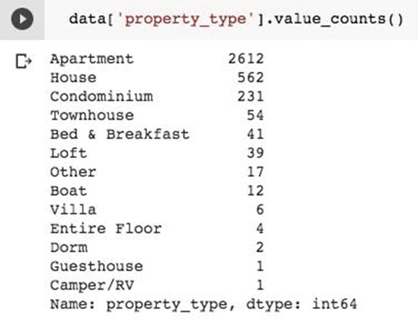
Frequency distribution for property_type values
Creating Datasets

Original price distribution

Price distribution after transformations
At this point, your data processing is complete. We now create the training and testing datasets.
We reserve 20% of our data for testing. The last thing that we need to do before building our estimator is to create Feature columns, which we do next.
Building Feature Columns
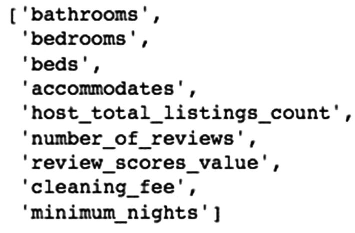
Numeric features array
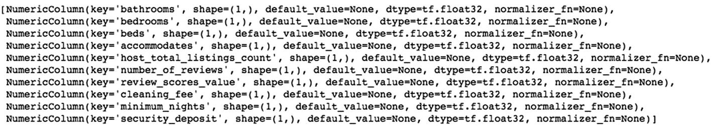
Features column

Categorical columns list
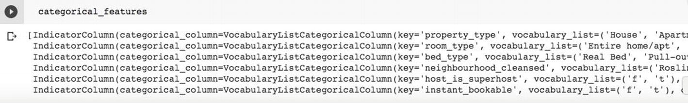
Features column for categorical columns
Defining Input Function
As seen in the previous project, the function takes features and labels as the first two parameters. The training parameter determines whether the data is to be used for training; if so, the data is shuffled. The from_tensor_slices function call creates a tensor for the data pipeline to our model. The function returns the data in batches.
Creating Estimator Instance
Note we use the LinearRegressor class as a premade estimator for regression. The first parameter is the Features columns, which specify the combined numerical and categorical columns list. The second parameter is the name of the directory where the logs would be maintained.
Model Training
The input function takes the features data in the xtrain dataset and the target values in the ytrain dataset. The training parameter is set to true that enables data shuffling. The number of steps would decide the number of epochs in the training phase.
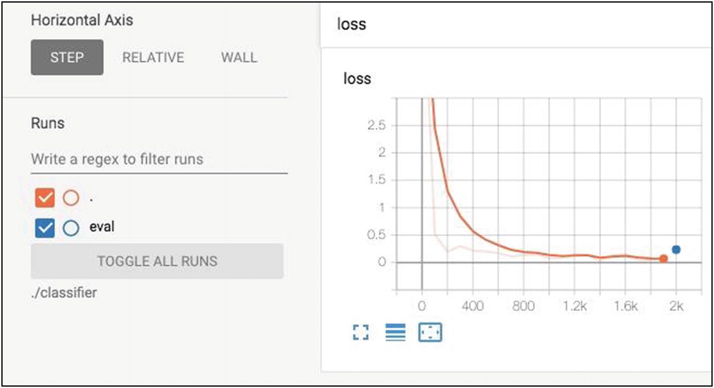
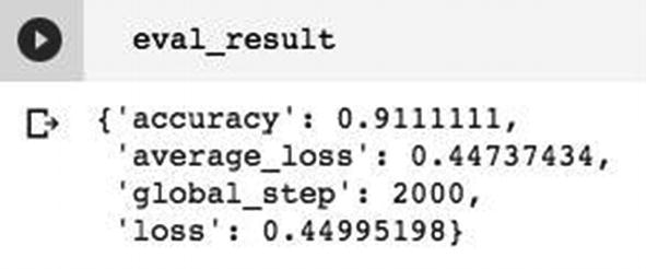
Model Evaluation

Loss metrics
Project Source
LinearRegressor-Estimator full source
This project has demonstrated how to use a premade LinearRegressor for solving the linear regression problems. Next, I will describe how to build a custom estimator of your own.
Custom Estimators
In the previous chapter, you developed a wine quality classifier. You used three different architectures – small, medium, and large – to compare their results. I will now show you how to convert these existing Keras models to a custom estimator to take advantage of the facilities provided by the estimator.
Creating Project
Loading Data
As you are already familiar with the data, I am not going to describe it again. I will not also include any data preprocessing here. I will straightaway move on to features selection.
Creating Datasets
Defining Model
The output consists of a single neuron which emits a float value for the wine quality. Note that we are treating this problem as a regression problem like the wine quality problem discussed in the previous chapter.
We consider this as a regression problem and thus use mse for our loss function. We will use this compiled model in the estimator instantiation. Before that, we define the input function.
Defining Input Function
The function definition is identical to the earlier example and does not need any further explanation.
Now, it is time for us to convert our model to the estimator.
Model to Estimator
The function takes two arguments; the first argument specifies the previously existing compiled Keras model, and the second argument specifies the folder name where the logs would be maintained during the training. The function call returns an estimator instance which you would use like in the earlier example to train, evaluate, and predict.
Model Training
For training, the input function takes the features data in xtrain and the labels in ytrain. The number of steps is set to 2000, which decides the number of training epochs. The mode set by the training argument takes the default value of True.
Evaluation
Note that we pick up the metrics from the earlier specified logs folder.
Project Source
ModelToEstimator full source
Custom Estimators for Pre-trained Models
In Chapter 4, you saw the use of pre-trained models from TF Hub. You have seen how to reuse these models in your own model definitions. It is also possible to convert these models into an estimator while extending their architecture. The following code shows you how to extend the VGG16 model and create a custom estimator on the extended model. VGG16 is a state-of-the-art deep learning which is trained to classify an image into 1000 categories. Suppose you just want to classify your datasets into just two categories – cats and dogs. So, we need just a binary classification. For this, we will need to change the output from categorical to binary. This example shows you how to replace the existing output layer of VGG16 with a single neuron Dense layer.
Creating Project
Importing VGG16
Building Your Model
We build a sequential model by taking the VGG16 as the base layer. On top of this, we add a pooling layer, followed by two Dense layers. The last layer is a binary output layer.
You may print the summaries of the two models to see the changes you have made.
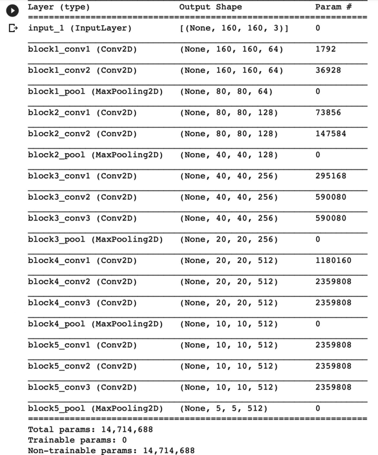
Model summary for VGG16
As you can see in Figure 6-24, the VGG16 models have several hidden layers, and the total number of trainable parameters equals more than 14 million. You can imagine the time and resources it would have taken to train this model. Obviously, in your application, when you use this model, you will never think of retraining this model.
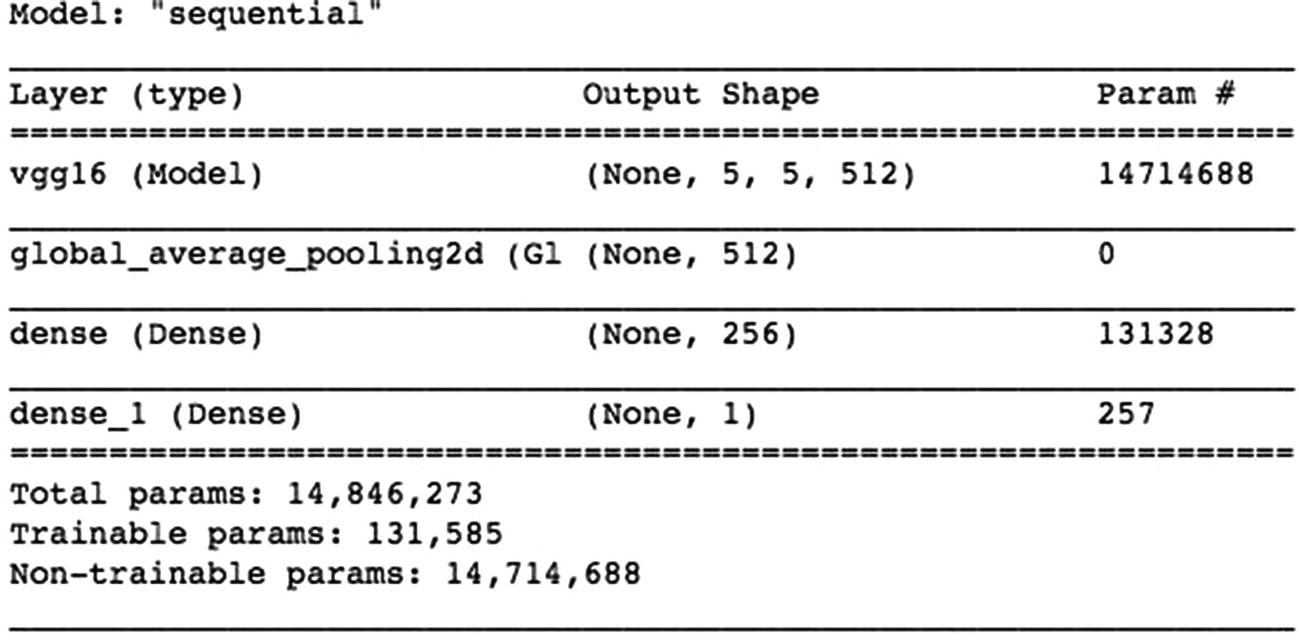
Model summary for the extended model
In your model, you have only about 100,000 trainable parameters.
Compiling Model
Creating Estimator
Before you train the estimator, you need to process your images.
Processing Data
Training/Evaluation
Note that I have used the same training dataset with a different step size for model evaluation, as no separate testing dataset is available for the purpose.
Project Source
VGG16-custom-estimator full source
This trivial example has demonstrated how you can use well-trained models into your own models.
Summary
The estimators facilitate model development by providing a unified interface for training, evaluation, and prediction. They provide a separation of data pipeline from the model development, thus allowing you to experiment with different datasets easily. The estimators are classified as premade and custom. In this chapter, you learned to use the premade estimators for both classification and regression types of problems. The custom estimators are used for migrating the existing models to the estimator interface to take advantage of the benefits offered by estimators. An estimator-based model can be trained on a distributed environment or even on a CPU/GPU/TPU. Once you develop your model using the estimator, it can be deployed easily even on a distributed environment without any code changes. You also learned to use a well-trained model like VGG16 in your own model building. It is recommended that you use the pre-trained model wherever possible. If it does not meet your purpose, then think of creating custom estimators.