© The Author(s), under exclusive license to APress Media, LLC, part of Springer Nature 2021
H. LuuBeginning Apache Spark 3https://doi.org/10.1007/978-1-4842-7383-8_4

4. Spark SQL: Advanced

Hien Luu1  
(1)
SAN JOSE, CA, USA
 

Chapter 3 introduced the foundational elements in the Spark SQL module, including the core abstraction, structured operations for manipulating structured data, and various supported data sources to read data from and write data to. Building on top of that foundation, this chapter covers some of the advanced capabilities in the Spark SQL module and peeks behind the curtain to understand the optimization and execution efficiency that the Catalyst optimizer and Tungsten engine provide. To help you with performing complex analytics, Spark SQL provides a set of powerful and flexible aggregation capabilities, the ability to join with multiple datasets, a large set of built-in and high-performant functions, an easy way to write your own custom function, and a set of advanced analytic functions. This chapter covers each of these topics in detail.

Aggregations

Performing any interesting and complex analytics on big data usually involves aggregation to summarize the data to extract patterns or insights or generate summary reports. Aggregations usually require grouping either on the entire dataset or based on one or more columns, and then apply aggregation functions such as summation, counting, or average to each group. Spark provides many commonly used aggregation functions and the ability to aggregate the values into a collection, which can then be further analyzed. The grouping of rows can be done at different levels, and Spark supports the following levels.
  • Treat a DataFrame as one group.

  • Divide a DataFrame into multiple groups using one or more columns and perform one or more aggregations on each group.

  • Divide a DataFrame into multiple windows and perform moving average, cumulative sum, or ranking. If a window is based on time, the aggregations can be done per tumbling or sliding windows.

Aggregation Functions

In Spark, all aggregations are done via functions. The aggregation functions are designed to perform aggregation on a set of rows, whether rows consist of all the rows or a subgroup of rows in a DataFrame. The documentation of the complete list of aggregation functions for the Scala language is available at http://spark.apache.org/docs/latest/api/scala/index.html#org.apache.spark.sql.functions$. For the Spark Python APIs, sometimes there are some gaps in the availability of some functions.

Common Aggregation Functions

This section describes a set of commonly used aggregation functions and provides examples of working with them. Table 4-1 describes the aggregation function. For a complete list, please see http://spark.apache.org/docs/latest/api/scala/index.html#org.apache.spark.sql.functions$.
Table 4-1

Commonly Used Aggregation Functions

Operation

Description

count(col)

Return the number of items per group.

countDistinct(col)

Return the unique number of items per group.

approx_count_distinct(col)

Return the approximate number of unique items per group.

min(col)

Return the minimum value of the given column per group.

max(col)

Return the maximum value of the given column per group.

sum(col)

Return the sum of the values in the given column per group.

sumDistinct(col)

Return the sum of the distinct values of the given column per group.

avg(col)

Return the average of the values of the given column per group.

skewness(col)

Return the skewness of the distribution of the values of the given column per group.

kurtosis(col)

Return the kurtosis of the distribution of the values of the given column per group.

variance(col)

Return the unbiased variance of the values of the given column per group.

stddev(col)

Return the standard deviation of the values of the given column per group.

collect_list(col)

Return a collection of values of the given column. The returned collection may contain duplicate values.

collect_set(col)

Return a collection of unique values of the given column.

To demonstrate the usage of these functions, let’s use the flight summary dataset, which is derived from the data files available on the Kaggle site at www.kaggle.com/usdot/flight-delays/data. This dataset contains the 2015 US domestic flight delays and cancellations. Listing 4-1 is the code for creating a DataFrame from this dataset.
val flight_summary = spark.read.format("csv")
                                           .option("header", "true")
                                           .option("inferSchema","true")
                                           .load("<path>/chapter5/data/flights/flight-summary.csv")
// use count action to find out number of rows in this dataset
flight_summary.count()
Long = 4693
Remember the count() function of the DataFrame is an action so it immediately returns a value to us. All the functions listed in Table 5-1 are lazily evaluated functions.
Below is the schema of the flight_summary dataset.
 |-- origin_code: string (nullable = true)
 |-- origin_airport: string (nullable = true)
 |-- origin_city: string (nullable = true)
 |-- origin_state: string (nullable = true)
 |-- dest_code: string (nullable = true)
 |-- dest_airport: string (nullable = true)
 |-- dest_city: string (nullable = true)
 |-- dest_state: string (nullable = true)
 |-- count: integer (nullable = true)
Listing 4-1

Create a DataFrame from Reading Flight Summary Dataset

Each row represents the flights from the origin_airport to dest_airport. The count column has the number of flights.

All the aggregation examples below are performing aggregation at the entire DataFrame level. Examples of performing aggregations at the subgroups level are given later in the chapter.

count(col)
Counting is a commonly used aggregation to find out the number of items in a group. Listing 4-2 computes the count for both the origin_airport and dest_airport columns, and as expected, the count is the same. To improve the readability of the result column, you can use the as function to give a friendlier column name. Note that you need to call the show action to see the result.
flight_summary.select(count("origin_airport"), count("dest_airport").as("dest_count")).show
+--------------------------+---------------+
|     count(origin_airport)|     dest_count|
+--------------------------+---------------+
|                      4693|           4693|
+--------------------------+---------------+
Listing 4-2

Computing the Count for Two Columns in the flight_summary DataFrame

When counting the number of items in a column, the count(col) function doesn’t include the null value in the count. To include the null value, the column name should be replaced with *. Listing 4-3 demonstrates this behavior by creating a small DataFrame with a null value in some columns.
import org.apache.spark.sql.Row
case class Movie(actor_name:String, movie_title:String, produced_year:Long)
val badMoviesDF = Seq( Movie(null, null, 2018L),
                       Movie("John Doe", "Awesome Movie", 2018L),
                       Movie(null, "Awesome Movie", 2018L),
                       Movie("Mary Jane", "Awesome Movie", 2018L)).toDF
badMoviesDF.show
+---------------+--------------------+-------------------+
|     actor_name|         movie_title|      produced_year|
+---------------+--------------------+-------------------+
|           null|                null|               2018|
|       John Doe|       Awesome Movie|               2018|
|           null|       Awesome Movie|               2018|
|      Mary Jane|       Awesome Movie|               2018|
+---------------+--------------------+-------------------+
// now performing the count aggregation on different columns
badMoviesDF.select(count("actor_name"), count("movie_title"), count("produced_year"), count("*")).show
+------------------+-------------------+---------------------+---------+
| count(actor_name)| count(movie_title)| count(produced_year)| count(1)|
+------------------+-------------------+---------------------+---------+
|                 2|                  3|                    4|        4|
+------------------+-------------------+---------------------+---------+
Listing 4-3

Counting Items with Null Value

The output table confirms that the count(col) function doesn’t include null the in the final count.

countDistinct(col)

This function does what it sounds like. It only counts the unique items per group. Listing 4-4 shows the differences in the count result between the countDistinct function and the count function . As it turns out, there are 322 unique airports in the flight_summary dataset.

flight_summary.select(countDistinct("origin_airport"), countDistinct("dest_airport"), count("*")).show
+-------------------------------+-----------------------------+----------+
| count(DISTINCT origin_airport)| count(DISTINCT dest_airport)|  count(1)|
+-------------------------------+-----------------------------+----------+
|                            322|                          322|      4693|
+-------------------------------+-----------------------------+----------+
approx_count_distinct (col, max_estimated_error=0.05)
Listing 4-4

Counting Unique Items in a Group

Counting the exact number of unique items in each group in a very large dataset is an expensive and time-consuming. In some use cases, it is sufficient to have an approximate unique count. One of those use cases is in the online advertising business, where there are hundreds of millions of ad impressions per hour. There is a need to generate a report on the number of unique visitors per certain type of member segment. Approximating a count of distinct items is a well-known problem in computer science. It is also known as the cardinality estimation problem .

Luckily, there is already a well-known algorithm called HyperLogLog (https://en.wikipedia.org/wiki/HyperLogLog) that you can use to solve this problem, and Spark has implemented a version of this algorithm in the approx_count_distinct function. Since the unique count is an approximation, there is a certain amount of error. This function allows you to specify the value for an acceptable estimation error for this use case. Listing 4-5 demonstrates the usage and behavior of the approx._count_distinct function . As you dial down the estimation error, it takes longer and longer for this function to complete and return the result.
// let's do the counting on the "count" column of flight_summary DataFrame.
// the default estimation error is 0.05 (5%)
flight_summary.select(count("count"),countDistinct("count"), approx_count_distinct("count", 0.05)).show
+--------------+----------------------+-----------------------------+
| count(count) | count(DISTINCT count)| approx_count_distinct(count)|
+--------------+----------------------+-----------------------------+
|          4693|                  2033|                         2252|
+--------------+----------------------+-----------------------------+
// to get a sense how much approx_count_distinct function is faster than countDistinct function,
// trying calling them separately
flight_summary.select(countDistinct("count")).show
// specify 1% estimation error
flight_summary.select(approx_count_distinct("count", 0.01)).show
// one my Mac laptop, the approx_count_distinct function took about 0.1 second and countDistinct function took 0.6 second.  The larger the approximation estimation error, the less time approx_count_distinct function takes to complete.
Listing 4-5

Counting Unique Items in a Group

min(col), max(col)
The minimum and maximum values of the items in a group are the two ends of a spectrum. These two functions are easy to understand and work with. Listing 4-6 extracts these two values from the count column.
flight_summary.select(min("count"), max("count")).show
+-------------+----------------+
|   min(count)|      max(count)|
+-------------+----------------+
|            1|           13744|
+-------------+----------------+
// looks like there is one very busy airport with 13744 incoming flights from another airport. It will be interesting  to find which airport
Listing 4-6

Get the Minimum and Maximum Values of the Count Column

sum(col)
This function computes the sum of the values in a numeric column. Listing 4-7 performs the sum of all the flights in the flight_summary dataset.
flight_summary.select(sum("count")).show
+---------------+
|     sum(count)|
+---------------+
|        5332914|
+---------------+
Listing 4-7

Using sum Function to Sum up the Count Values

sumDistinct(col)
This function does what it sounds like. It sums up only the distinct values of a numeric column. The sum of the distinct counts in the flight_summary DataFrame should be less than the total sum displayed in Listing 4-7. Listing 4-8 computes the sum of the distinct values.
flight_summary.select(sumDistinct("count")).show
+------------------------------+
|           sum(DISTINCT count)|
+------------------------------+
|                       3612257|
+------------------------------+
Listing 4-8

Using sumDistinct Function to Sum up the Distinct Count Values

avg(col)
This function calculates the average value of a numeric column. This convenient function simply takes the total and divides it by the number of items. Let’s see whether Listing 4-9 can validate the hypothesis.
flight_summary.select(avg("count"), (sum("count") / count("count"))).show
+--------------------------+------------------------------------+
|                avg(count)|         (sum(count) / count(count))|
+--------------------------+------------------------------------+
|        1136.3549968037503|                  1136.3549968037503|
+--------------------------+------------------------------------+
Listing 4-9

Computing the Average Value of the Count Column Using Two Different Ways

skewness(col), kurtosis(col)
In statistics, the distribution of the values in a dataset tells numerous stories behind the dataset. Skewness measures the symmetry of the value distribution in a dataset, and its value can be positive, zero, negative, or undefined. In a normal distribution or bell-shaped distribution, the skew value is 0. A positive skew indicates the tail on the right side is longer or fatter than the left side. A negative skew indicates the opposite, where the tail of the left side is longer or fatter than the right side. The tail of both sides is even when the skew is 0. Figure 4-1 shows an example of negative and positive skew.
../images/419951_2_En_4_Chapter/419951_2_En_4_Fig1_HTML.jpg
Figure 4-1

Negative and positive skew examples from https://en.wikipedia.org/wiki/Skewness

Kurtosis is a measure of the shape of the distribution curve, whether the curve is normal, flat, or pointy. Positive kurtosis indicates the curve is slender and pointy, and negative kurtosis indicates fat and flat. Listing 4-10 calculates the skewness and kurtosis for the count distribution in the flight_summary dataset.
flight_summary.select(skewness("count"), kurtosis("count")).show
+--------------------------+----------------------------+
|           skewness(count)|             kurtosis(count)|
+--------------------------+----------------------------+
|         2.682183800064101|           10.51726963017102|
+--------------------------+----------------------------+
Listing 4-10

Compute the Skewness and Kurtosis of Column Count

The result suggests the distribution of the counts is not symmetric, and the right tail is longer or fatter than the left tail. The kurtosis value suggests that the distribution curve is pointy.

variance(col), stddev(col)
In statistics, variance, and standard deviation measure the dispersion or the spread of the data. In other words, they tell the average distance of the values from the mean. When the variance value is low, the values are close to the mean. Variance and standard deviation are related; the latter is the square root of the former. Figure 4-2 shows samples from two populations with the same mean but different variances. The red population has a mean of 100 and a variance 100. The blue population has a mean of 100 and a variance of 2500. This example comes from https://en.wikipedia.org/wiki/Variance.
../images/419951_2_En_4_Chapter/419951_2_En_4_Fig2_HTML.jpg
Figure 4-2

Example of samples from two population from https://en.wikipedia.org/wiki/Variance

The variance and stddev calculate the variance and standard deviation, respectively. Spark provides two different implementations of these functions; one uses sampling to speed up the calculation, and the other uses the entire population. Listing 4-11 shows the variance and standard deviation of the count column in the flight_summary DataFrame .
// use the two variations of variance and standard deviation
flight_summary.select(variance("count"), var_pop("count"), stddev("count"), stddev_pop("count")).show
+-----------------+------------------+------------------+-----------------+
|   var_samp(count)|     var_pop(count)| stddev_samp(count)| stddev_pop(count)|
+-----------------+------------------+------------------+-----------------+
|1879037.7571558713| 1878637.3655604832|  1370.779981308405| 1370.633928355957|
+-----------------+------------------+------------------+-----------------+
Listing 4-11

Compute the Variance and Standard Deviation Using variance and sttdev Functions

It looks like the count values are pretty spread out in flight_summary DataFrame.

Aggregation with Grouping

This section covers aggregation with the grouping of one or more columns. The aggregations are usually performed on datasets that contain one or more categorical columns, which have low cardinality. Examples of categorical values are gender, age, city name, or country name. The aggregation is done through functions similar to the ones mentioned earlier. However, instead of performing aggregation on the global group in the DataFrame, they perform the aggregation on each subgroup.

Performing aggregation with grouping is a two-step process. The first step is to perform the grouping by using the groupBy(col1,col2,...) transformation, and that’s where you specify which columns to group the rows by. Unlike other transformations that return a DataFrame, the groupBy transformation returns an instance of RelationalGroupedDataset class, to which you can apply one or more aggregation functions. Listing 4-12 demonstrates a simple grouping of using one column and one aggregation. Notice the groupBy columns automatically be included in the output.
flight_summary.groupBy("origin_airport").count().show(5, false)
+------------------------------------------------------+-------+
|     origin_airport                                   |  count|
+------------------------------------------------------+-------+
|Melbourne International Airport                       |      1|
|San Diego International Airport (Lindbergh Field)     |     46|
|Eppley Airfield                                       |     21|
|Kahului Airport                                       |     18|
|Austin-Bergstrom International Airport                |     41|
+------------------------------------------------------+-------+
Listing 4-12

Grouping by origin_airport and Perform Count Aggregation

Listing 4-12 shows the flights out of Melbourne International Airport (Florida) go to only one other airport. However, the flights out of the Kahului Airport land at one of 18 other airports.

To make things a bit more interesting, let’s try grouping by two columns to calculate the same metric at the city level. Listing 4-13 shows how to do that.
flight_summary.groupBy('origin_state, 'origin_city).count().                  .where('origin_state === "CA").orderBy('count.desc).show(5)
+---------------+------------------+---------+
|   origin_state|       origin_city|    count|
+---------------+------------------+---------+
|             CA|     San Francisco|       80|
|             CA|       Los Angeles|       80|
|             CA|         San Diego|       47|
|             CA|           Oakland|       35|
|             CA|        Sacramento|       27|
+---------------+------------------+---------+
Listing 4-13

Grouping by origin_state and origin_city and Perform Count Aggregation

In addition to grouping by two columns, the statement filters the rows to only the ones with a “CA” state. The orderBy transformation makes it easy to identify which city has the greatest number of destination airports. It makes sense that both San Francisco and Los Angeles in California have the largest number of destination airports that one can fly to.

The RelationalGroupedDataset class provides a standard set of aggregation functions that you can use to apply to each subgroup. They are avg(cols), count(), mean(cols), min(cols), max(cols), sum(cols). Except for the count() function, all the remaining ones operate on numeric columns.

Multiple Aggregations per Group

Sometimes there is a need to perform multiple aggregations per group at the same time. For example, in addition to the count, you want to know the minimum and maximum values. The RelationalGroupedDataset class provides a very powerful function called agg that takes one or more column expressions, which means you can use any of the aggregation functions, including the ones listed in Table 4-1. One cool thing is these aggregation functions return an instance of the Column class, so you can then apply any of the column expressions using the provided functions. A common need is to rename the column after the aggregation is done to make it shorter, more readable, and easier to refer to. Listing 4-14 demonstrates how to do all of this.
import org.apache.spark.sql.functions._
flight_summary.groupBy("origin_airport")
                        .agg(
                                count("count").as("count"),
                                min("count"), max("count"),
                                sum("count")
                         ).show(5)
+--------------------+-------+----------+----------+------------+
|      origin_airport|  count|min(count)|max(count)|  sum(count)|
+--------------------+-------+----------+----------+------------+
|Melbourne Interna...|      1|      1332|      1332|        1332|
|San Diego Interna...|     46|         4|      6942|       70207|
|     Eppley Airfield|     21|         1|      2083|       16753|
|     Kahului Airport|     18|        67|      8313|       20627|
|Austin-Bergstrom ...|     41|         8|      4674|       42067|
+--------------------+-------+----------+----------+------------+
Listing 4-14

Multiple Aggregations After a Group by of origin_airport

By default, the aggregation column name is the aggregation expression, making the column name a bit long and difficult to refer to. Therefore, a common pattern is to use the Column.as function to rename the column to something more suitable.

The versatile agg function provides an additional way to express the column expressions via a string-based key-value map. The key is the column name, and the value is the aggregation method, which can be avg, max, min, sum, or count. Listing 4-15 provides an example of this approach.
flight_summary.groupBy("origin_airport")
                        .agg(
                                 "count" -> "count",
                                 "count" -> "min",
                                 "count" -> "max",
                                 "count" -> "sum")
                       .show(5)
Listing 4-15

Specifying Multiple Aggregations Using a Key-Value Map

The result is the same as the one from Listing 4-14. Notice there isn’t an easy to rename the aggregation result column name. One advantage this approach has over the first one is the map can programmatically be generated. When writing production ETL jobs or performing exploratory analysis, the first approach is used more often than the second one.

Collection Group Values

The collect_list(col) and collect_set(col) functions are useful to collect all the values of a particular group after the grouping is applied. Once the values of each group are placed in a collection, there is freedom to operate them any way you choose. There is one small difference in the returned collection of these functions, which is the uniqueness. The collection_list function returns a collection containing duplicate values, and the collection_set function returns a collection containing unique values. Listing 4-16 shows using the collection_list function to collect the destination cities with more than 5500 flights coming into them from each origin state.
val highCountDestCities = flight_summary.where('count > 5500)
                               .groupBy("origin_state")
                               .agg(collect_list("dest_city")
                               .as("dest_cities"))
highCountDestCities.withColumn("dest_city_count",
                               size('dest_cities))
                   .show(5, false)
+------------+------------------------------------+----------------+
|origin_state|         dest_cities                | dest_city_count|
+------------+------------------------------------+----------------+
|          AZ|      [Seattle, Denver, Los Angeles]|               3|
|          LA|      [Atlanta]                     |               1|
|          MN|      [Denver, Chicago]             |               2|
|          VA|      [Chicago, Boston, Atlanta]    |               3|
|          NV|[Denver, Los Angeles, San Francisco]|               3|
+------------+------------------------------------+----------------+
Listing 4-16

Using collection_list to Collect High Traffic Destination Cities Per Origin State

Aggregation with Pivoting

Pivoting is a way to summarize the data by specifying one of the categorical columns and then performing aggregations on other columns so that the categorical values are transposed from rows into individual columns. Another way of thinking about pivoting is that it is a way to translate rows into columns while applying one or more aggregations. This technique is commonly used in data analysis or reporting. The pivoting process starts with grouping one or more columns, pivots on a column, and finally ends with applying one or more aggregations on one or more columns.

Listing 4-17 shows a pivoting example on a small dataset of students where each row contains the student’s name, gender, weight, and graduation year. Pivoting makes it easy to compute the average weight of each gender for each graduation year.
import org.apache.spark.sql.Row
case class Student(name:String, gender:String, weight:Int, graduation_year:Int)
val studentsDF = Seq(Student("John", "M", 180, 2015),
                     Student("Mary", "F", 110, 2015),
                     Student("Derek", "M", 200, 2015),
                     Student("Julie", "F", 109, 2015),
                     Student("Allison", "F", 105, 2015),
                     Student("kirby", "F", 115, 2016),
                     Student("Jeff", "M", 195, 2016)).toDF
// calculating the average weight for gender per graduation year
studentsDF.groupBy("graduation_year").pivot("gender")
                                     .avg("weight").show()
+----------------+------+---------+
| graduation_year|     F|        M|
+----------------+------+---------+
|            2015| 108.0|    190.0|
|            2016| 115.0|    195.0|
+----------------+------+---------+
Listing 4-17

Pivoting on a Small Dataset

This example has only one aggregation, and the gender categorical column has only two possible unique values; therefore, the result table has only two columns. If the gender column has three possible unique values, there are three columns in the result table. You can leverage the agg function to perform multiple aggregations, creating more columns in the result table. Listing 4-18 is an example of performing multiple aggregations on the DataFrame from Listing 4-17.
studentsDF.groupBy("graduation_year").pivot("gender")
                  .agg(
                          min("weight").as("min"),
                          max("weight").as("max"),
                          avg("weight").as("avg")
                  ).show()
+---------------+------+-------+-------+-------+-------+------+
|graduation_year| F_min|  F_max|  F_avg|  M_min|  M_max| M_avg|
+---------------+------+-------+-------+-------+-------+------+
|           2015|   105|    110|  108.0|    180|    200| 190.0|
|           2016|   115|    115|  115.0|    195|    195| 195.0|
+---------------+------+-------+-------+-------+-------+------+
Listing 4-18

Multiple Aggregations After Pivoting

The number of columns added after the group columns in the result table is the product of the number of unique values of the pivot column and the number of aggregations.

If the pivoting column has a lot of distinct values, you can selectively choose which values to generate the aggregations for. Listing 4-19 shows how to specify values to the pivoting function.
studentsDF.groupBy("graduation_year").pivot("gender", Seq("M"))
                  .agg(
                          min("weight").as("min"),
                          max("weight").as("max"),
                          avg("weight").as("avg")
                  ).show()
+---------------------+---------+----------+---------+
|      graduation_year|    M_min|     M_max|    M_avg|
+---------------------+---------+----------+---------+
|                 2015|      180|       200|    190.0|
|                 2016|      195|       195|    195.0|
+---------------------+---------+----------+---------+
Listing 4-19

Selecting Values of Pivoting Column to Generate the Aggregations For

Specifying a list of distinct values for the pivot column speeds up the pivoting process. Otherwise, Spark spends some effort in figuring out a list of distinct values on its own.

Joins

To perform any kind of complex and interesting data analysis or manipulations, you often need to bring together the data from multiple datasets through the process of joining. This is a well-known technique in SQL parlance. Performing a join combines the columns of two datasets (could be different or same), and the combined dataset contains columns from both sides. This enables you to further analyze the combined dataset so that it is not possible with each set. Let’s take an example of the two datasets from an online e-commerce company. One represents the transactional data that contains information about which customers purchased what products (a.k.a. fact table). The other one represents the information on each customer (a.k.a. dimension table). By joining these two datasets, you can extract insights about which products are more popular with certain segments of customers in terms of age or location.

This section covers how to perform joining in Spark SQL using the join transformation and the various types of join it supports. The last portion of this section describes how Spark SQL internally performs the joining.

Note

In the world of performing data analysis using SQL, a join is a technique used quite often. If you are new to SQL, it is highly recommended that you learn the fundamental concepts and the different kinds of join at https://​en.​wikipedia.​org/​wiki/​Join_​(SQL). A few tutorials about joins are provided at www.w3schools.com/sql/sql_join.asp.

Join Expression and Join Types

Performing a join of two datasets requires you to specify two pieces of information. The first one is a join expression that specifies which columns from each side should determine which rows from both datasets are included in the joined dataset. The second one is the join type, which determines what should be included in the joined dataset. Table 4-2 provides a list of supported join types in Spark SQL.
Table 4-2

Join Types

Type

Description

Inner join (a.k.a. equi-join)

Return rows from both datasets when the join expression evaluates to true.

Left outer join

Return rows from the left dataset even when the join expression evaluates as false.

Right outer join

Return rows from the right dataset even when the join expression evaluates as false.

Outer join

Return rows from both datasets even when the join expression evaluates as false.

Left anti-join

Return rows only from the left dataset when the join expression evaluates as false.

Left semi-join

Return rows only from the left dataset when the join expression evaluates to true.

Cross

(a.k.a. Cartesian)

Return rows by combining each row from the left dataset with each row in the right dataset. The number of rows is a product of the size of each dataset.

To help visualize some of the join types, Figure 4-3 shows a set of Venn diagrams for the common join types from https://en.wikipedia.org/wiki/Join_ (SQL)#Outer_join.
../images/419951_2_En_4_Chapter/419951_2_En_4_Fig3_HTML.jpg
Figure 4-3

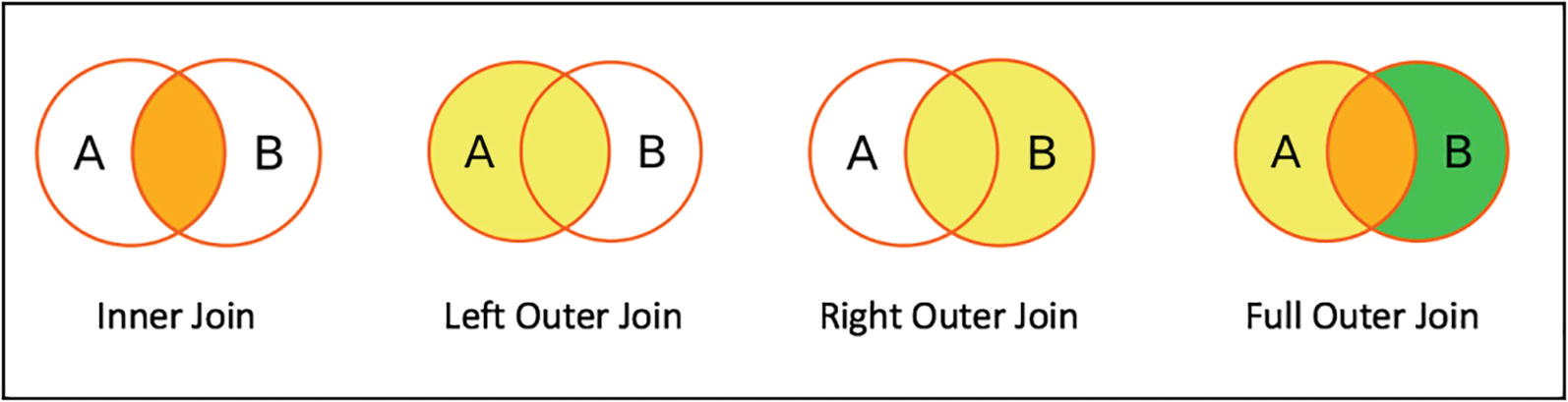
Venn diagrams for common join types

Working with Joins

I used two small DataFrames to demonstrate how to perform joining in Sparking SQL. The first one represents a list of employees, and each row contains the employee’s name and the department they belong to. The second one contains a list of departments, and each row contains a department ID and department name. Listing 4-20 contains a snippet of code to create these two DataFrames.
case class Employee(first_name:String, dept_no:Long)
val employeeDF = Seq( Employee("John", 31),
                      Employee("Jeff", 33),
                      Employee("Mary", 33),
                      Employee("Mandy", 34),
                      Employee("Julie", 34),
                      Employee("Kurt", null.asInstanceOf[Int])
                     ).toDF
case class Dept(id:Long, name:String)
val deptDF = Seq( Dept(31, "Sales"),
                  Dept(33, "Engineering"),
                  Dept(34, "Finance"),
                  Dept(35, "Marketing")
                 ).toDF
// register them as views so we can use SQL for perform joins
employeeDF.createOrReplaceTempView("employees")
deptDF.createOrReplaceTempView("departments")
Listing 4-20

Creating Two Small DataFrames to Use in the Following Join Type Examples

Inner Joins

This is the most used join type with the join expression containing the equality comparison of the columns from both datasets. The joined dataset contains the rows only when the join expression is evaluated to be true; in other words, the join column values are the same in both datasets. Rows that don’t have matching column values are excluded from the joined dataset. If the join expression uses the equality comparison, then the number of rows in the joined table only be as large as the size of the smaller dataset. The inner join is the default join type in Spark SQL, so it is optional to specify it in the join transformation. Listing 4-21 provides examples of doing an inner join .
// define the join expression of equality comparison
val deptJoinExpression = employeeDF.col("dept_no") === deptDF.col("id")
// perform the join
employeeDF.join(deptDF, joinExpression, "inner").show
// no need to specify the join type since "inner" is the default
employeeDF.join(deptDF, joinExpression).show
+-------------+----------+---+----------------+
|   first_name|   dept_no| id|            name|
+-------------+----------+---+----------------+
|         John|        31| 31|           Sales|
|         Jeff|        33| 33|     Engineering|
|         Mary|        33| 33|     Engineering|
|        Mandy|        34| 34|         Finance|
|        Julie|        34| 34|         Finance|
+-------------+----------+---+----------------+
// using SQL
spark.sql("select * from employees JOIN departments on dept_no == id").show
Listing 4-21

Performing Inner Join by the Department ID

As expected, the joined dataset contains only the rows with matching department IDs from both employee and department datasets and the columns from both datasets. The output tells you exactly which department each employee belongs to.

The join expression can be specified in the join transformation or using the where transformation. If the column names are unique, it is possible to refer to the columns in the join expression using a short-handed version. If not, you must specify which DataFrame a particular column comes from using the col function. Listing 4-22 shows different ways of expressing a join expression.
// a shorter version of the join expression
employeeDF.join(deptDF, 'dept_no === 'id).show
// specify the join expression inside the join transformation
employeeDF.join(deptDF, employeeDF.col("dept_no") === deptDF.col("id")).show
// specify the join expression using the where transformation
employeeDF.join(deptDF).where('dept_no === 'id).show
Listing 4-22

Different Ways of Expressing a Join Expression

Join expression is simply a Boolean predicate, and therefore it can be as simple as comparing two columns or as complex as chaining multiple logical comparisons of pairs of columns .

Left Outer Joins

The joined dataset of this join type includes all the rows from an inner join plus all the rows from the left dataset that the join expression is evaluated as false. For those nonmatching rows, it fills in a NULL value for the columns of the right dataset. Listing 4-23 is an example of doing a left outer join.
// the join type can be either "left_outer" or "leftouter"
employeeDF.join(deptDF, 'dept_no === 'id, "left_outer").show
// using SQL
spark.sql("select * from employees LEFT OUTER JOIN departments on dept_no == id").show
+--------------+----------+----+----------------+
|    first_name|   dept_no|  id|            name|
+--------------+----------+----+----------------+
|          John|        31|  31|           Sales|
|          Jeff|        33|  33|     Engineering|
|          Mary|        33|  33|     Engineering|
|         Mandy|        34|  34|         Finance|
|         Julie|        34|  34|         Finance|
|          Kurt|         0|null|            null|
+--------------+----------+----+----------------+
Listing 4-23

Performing a Left Outer Join

As expected, the marketing department doesn’t have any matching rows from the employee dataset. The joined dataset tells you the department that an employee is assigned to and which departments have no employees .

Right Outer Joins

The behavior of this join type resembles the behavior of the left outer join type, except the same treatment is applied to the right dataset. In other words, the joined dataset includes all the rows from an inner join plus all the rows from the right dataset that the join expression evaluates as false. Listing 4-24 is an example of doing a right outer join.
employeeDF.join(deptDF, 'dept_no === 'id, "right_outer").show
// using SQL
spark.sql("select * from employees RIGHT OUTER JOIN departments on dept_no == id").show
+-------------+-----------+----+----------------+
|   first_name|    dept_no|  id|            name|
+-------------+-----------+----+----------------+
|         John|         31|  31|           Sales|
|         Mary|         33|  33|     Engineering|
|         Jeff|         33|  33|     Engineering|
|        Julie|         34|  34|         Finance|
|        Mandy|         34|  34|         Finance|
|         null|       null|  35|       Marketing|
+-------------+-----------+----+----------------+
Listing 4-24

Performing a Right Outer Join

As expected, the marketing department doesn’t have any match rows from the employee dataset. The joined dataset tells you the department that an employee is assigned to and which departments have no employees.

Outer Joins (a.k.a. Full Outer Joins)

The behavior of this join type is effectively the same as combining the result of both the left outer join and the right outer join. Listing 4-25 is an example of doing an outer join.
employeeDF.join(deptDF, 'dept_no === 'id, "outer").show
// using SQL
spark.sql("select * from employees FULL OUTER JOIN departments on dept_no == id").show
+-------------+-----------+----+----------------+
|   first_name|    dept_no|  id|            name|
+-------------+-----------+----+----------------+
|         Kurt|          0|null|            null|
|        Mandy|         34|  34|         Finance|
|        Julie|         34|  34|         Finance|
|         John|         31|  31|           Sales|
|         Jeff|         33|  33|     Engineering|
|         Mary|         33|  33|     Engineering|
|         null|       null|  35|       Marketing|
+-------------+-----------+----+----------------+
Listing 4-25

Performing an Outer Join

The result from the outer join allows you to see which department an employee is assigned to and which departments have employees and which employees are not assigned to a department and which departments don’t have any employees.

Left Anti-Joins

This join type lets you find out which rows from the left dataset don’t have any matching rows on the right dataset, and the joined dataset contains only the columns from the left dataset. Listing 4-26 is an example of doing a left anti-join .
employeeDF.join(deptDF, 'dept_no === 'id, "left_anti").show
// using SQL
spark.sql("select * from employees LEFT ANTI JOIN departments on dept_no == id").show
+-------------+-----------+
|   first_name|    dept_no|
+-------------+-----------+
|         Kurt|          0|
+-------------+-----------+
Listing 4-26

Performing a Left Anti-Join

The result from the left anti-join can easily tell you which employees are not assigned to a department. Notice the right anti-join type doesn’t exist; however, you can easily switch the datasets around to achieve the same goal .

Left Semi-Joins

The behavior of this join type is similar to the inner join type, except the joined dataset doesn’t include the columns from the right dataset. Another way of thinking about this join type is its behavior is the opposite of the left anti-join, where the joined dataset contains only the matching rows. Listing 4-27 is an example of doing a left semi-join .
employeeDF.join(deptDF, 'dept_no === 'id, "left_semi").show
// using SQL
spark.sql("select * from employees LEFT SEMI JOIN departments on dept_no == id").show
+-------------+-----------+
|   first_name|    dept_no|
+-------------+-----------+
|         John|         31|
|         Jeff|         33|
|         Mary|         33|
|        Mandy|         34|
|        Julie|         34|
+-------------+-----------+
Listing 4-27

Performing a Left Semi-Join

Cross (a.k.a. Cartesian)

In terms of usage, this join type is the simplest to use because the join expression is not needed. Its behavior can be a bit dangerous because it joins every single row in the left dataset with every row in the right dataset. The size of the joined dataset is the product of the size of the two datasets. For example, if each dataset size is 1024, then the size of the joined dataset is over 1 million rows. For this reason, the way to use this join type is by explicitly using a dedicated transformation in the DataFrame class, rather than specifying this join type as a string. Listing 4-28 is an example of doing a cross join .
// using crossJoin transformation and display the count
employeeDF.crossJoin(deptDF).count
Long = 24
// using SQL and passing 30 value to show action to see all rows
spark.sql("select * from employees CROSS JOIN departments").show(30)
+-------------+----------+---+----------------+
|   first_name|   dept_no| id|            name|
+-------------+----------+---+----------------+
|         John|        31| 31|           Sales|
|         John|        31| 33|     Engineering|
|         John|        31| 34|         Finance|
|         John|        31| 35|       Marketing|
|         Jeff|        33| 31|           Sales|
|         Jeff|        33| 33|     Engineering|
|         Jeff|        33| 34|         Finance|
|         Jeff|        33| 35|       Marketing|
|         Mary|        33| 31|           Sales|
|         Mary|        33| 33|     Engineering|
|         Mary|        33| 34|         Finance|
|         Mary|        33| 35|       Marketing|
|        Mandy|        34| 31|           Sales|
|        Mandy|        34| 33|     Engineering|
|        Mandy|        34| 34|         Finance|
|        Mandy|        34| 35|       Marketing|
|        Julie|        34| 31|           Sales|
|        Julie|        34| 33|     Engineering|
|        Julie|        34| 34|         Finance|
|        Julie|        34| 35|       Marketing|
|         Kurt|         0| 31|           Sales|
|         Kurt|         0| 33|     Engineering|
|         Kurt|         0| 34|         Finance|
|         Kurt|         0| 35|       Marketing|
+-------------+----------+---+----------------+
Listing 4-28

Performing a Cross Join

Dealing with Duplicate Column Names

From time to time, two DataFrames might have one or more columns with the same name. Before joining them, it is best to rename those columns in one of the two DataFrames to avoid access ambiguity issues; otherwise, the joined DataFrame would have multiple columns with the same name. Listing 4-29 simulates this situation.
// add a new column to deptDF with name dept_no
val deptDF2 = deptDF.withColumn("dept_no", 'id)
deptDF2.printSchema
 |-- id: long (nullable = false)
 |-- name: string (nullable = true)
 |-- dept_no: long (nullable = false)
// now employeeDF with deptDF2 using dept_no column
val dupNameDF = employeeDF.join(deptDF2, employeeDF.col("dept_no") === deptDF2.col("dept_no"))
dupNameDF.printSchema
 |-- first_name: string (nullable = true)
 |-- dept_no: long (nullable = false)
 |-- id: long (nullable = false)
 |-- name: string (nullable = true)
 |-- dept_no: long (nullable = false)
Listing 4-29

Simulate a Joined DataFrame with Multiple Names That Are the Same

Notice the dupNameDF DataFrame now has two columns with the same name, dept_no. Spark throws an error when you project the dupNameDF DataFrame using the dept_no in Listing 4-30.
dupNameDF.select("dept_no")
org.apache.spark.sql.AnalysisException: Reference 'dept_no' is ambiguous, could be: dept_no#30L, dept_no#1050L.;
Listing 4-30

Projecting Column dept_no in the dupNameDF DataFrame

As it turns out, there are several ways to deal with this issue.

Use Original DataFrame

The joined DataFrame remembers which columns come from which original DataFrame during the joining process. To disambiguate which DataFrame a column comes from, you can just tell Spark to prefix it with its original DataFrame name. Listing 4-31 shows how to do this.
dupNameDF.select(deptDF2.col("dept_no"))
Listing 4-31

Using the Original DataFrame deptDF2 to Refer to dept_no Column in the Joined DataFrame

Renaming Column Before Joining

Another approach to avoid a column name ambiguity issue is to rename a column in one of the DataFrames using the withColumnRenamed transformation . Since this is simple, I leave it as an exercise for you.

Using Joined Column Name

When the joined column name is the same in both DataFrames, you can leverage a version of the join transformation that automatically removes the duplicate column name in the joined DataFrame. However, if it was a self-join, meaning joining a DataFrame to itself, then there is no way to refer to other duplicate column names. In that case, you need to use the column renaming technique. Listing 4-32 shows an example of performing a join using a joined column name.
val noDupNameDF = employeeDF.join(deptDF2, "dept_no")
noDupNameDF.printSchema
 |-- dept_no: long (nullable = false)
 |-- first_name: string (nullable = true)
 |-- id: long (nullable = false)
 |-- name: string (nullable = true)
Listing 4-32

Performing a Join Using Joined Column Name

Notice there is only one dept_no column in the noDupNameDF DataFrame.

Overview of Join Implementation

Joining is one of the most complex and expensive operations in Spark. At a high level, there are a few strategies Spark uses to perform the joining of two datasets. They are shuffle hash join and broadcast join. The main criteria for selecting a particular strategy are based on the size of the two datasets. When the size of both datasets is large, then the shuffle hash join strategy is used. When the size of one of the datasets is small enough to fit into the memory of the executor, then the broadcast join strategy is used. The following sections go into detail on how each joining strategy works.

Shuffle Hash Join

Conceptually, joining is about combining the rows of two datasets that meet the condition in the join expression. To do that, rows with the same column values need to be transferred across the network, co-located on the same partition.

The shuffle hash join implementation consists of two steps. The first step computes the hash value of the column(s) in the join expression of each row in each dataset and then shuffles those rows with the same hash value to the same partition. To determine which partition a particular row is moved to, Spark performs a simple arithmetic operation, which computes the modulo of the hash value by the number of partitions. The second step combines the columns of those rows that have the same column hash value. At the high level, these two steps are like the steps in the MapReduce programming model.
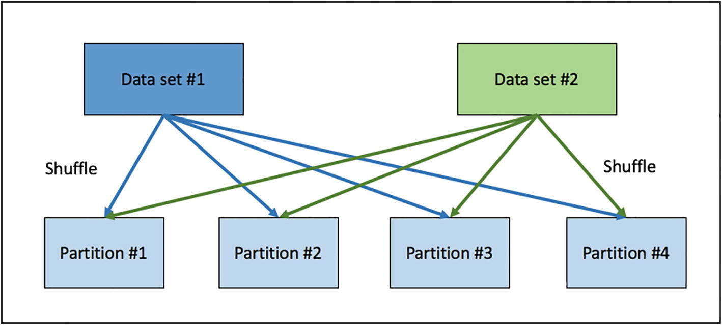
Figure 4-4 shows the shuffling going on in the shuffle hash join. It is an expensive operation due to transferring a large amount of data from across machines over the network. When moving data across a network, the data usually goes through a serialization and deserialization process. Imagine performing a join on two large datasets where the size of each one is 100 GB. In this scenario, it moves approximately 200GB of data around. It is not possible to completely avoid a shuffle hash join when joining two large datasets. Still, it is important to be mindful about reducing the frequency of joining them whenever possible.
../images/419951_2_En_4_Chapter/419951_2_En_4_Fig4_HTML.jpg
Figure 4-4

Shuffle hash join

Broadcast Hash Join

This join strategy is applicable when one of the datasets is small enough to fit into memory. Knowing that the shuffle hash join is an expensive operation, the broadcast hash join avoids shuffling both datasets and shuffles only the smaller one. Like the shuffle hash join strategy, this one also consists of two steps. The first step is to broadcast a copy of the smaller dataset to each of the larger dataset’s partitions. The second step is to iterate through each row in the larger dataset and look up the corresponding rows in the smaller dataset with match column values. Figure 4-5 shows the broadcasting of the small dataset.
../images/419951_2_En_4_Chapter/419951_2_En_4_Fig5_HTML.jpg
Figure 4-5

Broadcast hash join

It is easy to understand that a broadcast hash join is preferred when it is applicable. For the most part, Spark SQL can automatically figure out when to use broadcast hash join or shuffle hash join based on the statistics it has about datasets while reading them. However, it is feasible to provide a hint to Spark SQL to use broadcast hash join when using the join transformation. Listing 4-33 provides an example of doing that.
import org.apache.spark.sql.functions.broadcast
// Use broadcast hash join strategy and print out execution plan
employeeDF.join(broadcast(deptDF), employeeDF.col("dept_no") === deptDF.col("id")).explain()
// User broadcast hash join hint in a SQL statement
spark.sql("select /*+ MAPJOIN(departments) */ * from employees JOIN departments on dept_no == id").explain()
== Physical Plan ==
*BroadcastHashJoin [dept_no#30L], [id#41L], Inner, BuildRight
:- LocalTableScan [first_name#29, dept_no#30L]
+- BroadcastExchange HashedRelationBroadcastMode(List(input[0, bigint, false]))
   +- LocalTableScan [id#41L, name#42]
Listing 4-33

Provide a Hint to Use Broadcast Hash Join

Functions

The DataFrame APIs are designed to operate or transform individual rows in a dataset, such as filtering and grouping. If you want to transform the column value of each row, such as converting a string from uppercase to camel case, you use a function. Functions are methods that are applied to columns. Spark SQL provides a large set of commonly needed functions and an easy way to create new ones. Approximately 30 new built-in functions were added in Spark 3.0 version.

Working with Built-in Functions

To be effective and productive at using Spark SQL to perform distributed data manipulations, you must be proficient at working with Spark SQL built-in functions . These built-in functions are designed to generate optimized code for execution at runtime, so it is best to take advantage of them before coming up with your own functions. One commonality among these functions is they are designed to take one or more columns of the same row as the input, and they return only a single column as the output. Spark SQL provides more than 200 built-in functions, and they are grouped into different categories. These functions can be used in DataFrame operations, such as select, filter, and groupBy.

For a complete list of built-in functions, refer to the Spark API Scala documentation at https://spark.apache.org/docs/latest/api/scala/org/apache/spark/sql/functions$.html. Table 4-3 classifies them into different categories.
Table 4-3

A Subset of Built-in Functions for Each Category

Category

Description

Date time

unix_timestamp, from_unixtime, to_date, current_date, current_timesatmp, date_add, date_sub, add_months, datediff, months_between, dayofmonth, dayofyear, weekofyear, second, minute, hour, month, make_date, make_timestamp, make_interval

String

concat, length, levenshtein, locate, lower, upper, ltrim, rtrim, trim, lpad, rpad, repeat, reverse, split, substring, base64

Math

cos, acos, sin, asin, tan, atan, ceil, floor, exp, factorial, log, pow, radian, degree, sqrt, hex, unhex

Cryptography

cr32, hash, md5, sha1, sha2

Aggregation

approx._count_distinct, countDistinct, sumDistinct, avg, corr, count, first, last, max, min, skewness, sum,

Collection

array_contain, explode, from_json, size, sort_array, to_json, size

Window

dense_rank, lag, lead, ntile, rank, row_number

Misc.

coalesce, isNan, isnull, isNotNull, monotonically_increasing_id, lit, when

Most of these functions are easy to understand and straightforward to use. The following sections provide working examples of some of the interesting ones.

Working with Date Time Functions

The more you use Spark to perform data analysis, the more chance you encounter datasets that have one more date or time-related columns. The Spark built-in data time functions broadly fall into the following three categories: converting the date or timestamp from one format to another, performing a data-time calculation, and extracting specific values from a date or timestamp, such as year, month, day of the week, and so on.

The date-time conversion functions help convert a time string into either a date, timestamp, or Unix timestamp and vice versa. Internally, it uses the Java date format pattern syntax, which is documented at http://docs.oracle.com/javase/tutorial/i18n/format/simpleDateFormat.html. The default date format these functions use is yyyy-MM-dd HH:mm:ss. Therefore, if your date or timestamp column’s date format is different, you need to provide that pattern to these conversion functions. Listing 4-34 shows an example of converting date and timestamp in string type to Spark date and timestamp type.
// the last two columns don't follow the default date format
val testDF = Seq((1, "2018-01-01", "2018-01-01 15:04:58:865",
                  "01-01-2018", "12-05-2017 45:50"))
                 .toDF("id", "date", "timestamp", "date_str",
                       "ts_str")
// convert these strings into date, timestamp and unix timestamp
// and specify a custom date and timestamp format
val testResultDF = testDF.select(to_date('date).as("date1"),
                           to_timestamp('timestamp).as("ts1"),
                     to_date('date_str,"MM-dd-yyyy").as("date2"),
             to_timestamp('ts_str, "MM-dd-yyyy mm:ss").as("ts2"),
             unix_timestamp('timestamp).as("unix_ts"))
                     .show(false)
// date1 and ts1 are of type date and timestamp respectively
testResultDF.printSchema
 |-- date1: date (nullable = true)
 |-- ts1: timestamp (nullable = true)
 |-- date2: date (nullable = true)
 |-- ts2: timestamp (nullable = true)
 |-- unix_ts: long (nullable = true)
testDateResultDF.show
+----------+-------------------+----------+-------------------+-----------+
|     date1|                ts1|     date2|                ts2|    unix_ts|
+----------+-------------------+----------+-------------------+-----------+
|2018-01-01|2018-01-01 15:04:58|2018-01-01|2017-12-05 00:45:50| 1514847898|
+----------+-------------------+----------+-------------------+-----------+
Listing 4-34

Converting date and timestamp String to Spark Date and Timestamp Type

It is just as easy to convert a date or timestamp to a time string by using the date_format function with a custom date format or using the from_unixtime function to convert a Unix timestamp (in seconds) to a time string. Listing 4-35 shows examples of the conversions .
testResultDF.select(date_format('date1,"dd-MM-YYYY").as("date_str"),date_format('ts1, "dd-MM-YYYY HH:mm:ss").as("ts_str"),
 from_unixtime('unix_ts,"dd-MM-YYYY HH:mm:ss").as("unix_ts_str"))
                 .show
+-------------+------------------------+------------------------+
|     date_str|                  ts_str|             unix_ts_str|
+-------------+------------------------+------------------------+
|   01-01-2018|     01-01-2018 15:04:58|     01-01-2018 15:04:58|
+-------------+------------------------+------------------------+
Listing 4-35

Converting Date, Timestamp, and Unix Timestamp to Time String

The date-time calculation functions are useful for figuring out the difference between two dates or timestamps and the ability to perform date or time arithmetic. Listing 4-36 shows working examples of date-time calculation .
val employeeData = Seq(("John", "2016-01-01", "2017-10-15"),
                       ("May", "2017-02-06", "2017-12-25"))
                       .toDF("name", "join_date", "leave_date")
employeeData.show
+------+----------------+--------------+
|  name|       join_date|    leave_date|
+------+----------------+--------------+
|  John|      2016-01-01|    2017-10-15|
|   May|      2017-02-06|    2017-12-25|
+------+----------------+--------------+
// perform date and month calculations
employeeData.select('name,
            datediff('leave_date, 'join_date).as("days"),
            months_between('leave_date, 'join_date).as("months"),
            last_day('leave_date).as("last_day_of_mon"))
             .show
+------+------+----------------+-----------------------+
|  name|  days|          months|        last_day_of_mon|
+------+------+----------------+-----------------------+
|  John|   653|      21.4516129|             2017-10-31|
|   May|   322|     10.61290323|             2017-12-31|
+------+------+----------------+-----------------------+
// perform date addition and subtraction
val oneDate = Seq(("2018-01-01")).toDF("new_year")
oneDate.select(date_add('new_year, 14).as("mid_month"),
               date_sub('new_year, 1).as("new_year_eve"),
               next_day('new_year, "Mon").as("next_mon"))
        .show
+--------------+--------------------+----------------+
|     mid_month|        new_year_eve|        next_mon|
+--------------+--------------------+----------------+
|    2018-01-15|          2017-12-31|      2018-01-08|
+--------------+--------------------+----------------+
Listing 4-36

Date Time Calculation Examples

The ability to extract specific fields from a date or timestamp value such as year, month, hour, minutes, and seconds is convenient. For example, when there is a need to group all the stock transactions by quarter, month, or week, you can just extract that information from the transaction date and group by those values. Listing 4-37 shows how easy it is to extract fields out of a date or timestamp .
val valentimeDateDF = Seq(("2018-02-14 05:35:55")).toDF("date")
valentimeDateDF.select(year('date).as("year"),
                       quarter('date).as("quarter"),
                       month('date).as("month"),
                       weekofyear('date).as("woy"),
                       dayofmonth('date).as("dom"),
                       dayofyear('date).as("doy"),
                       hour('date).as("hour"),
                       minute('date).as("minute"),
                       second('date).as("second"))
                .show
+-----+--------+------+-----+-----+-----+------+-------+--------+
| year| quarter| month|  woy|  dom|  doy|  hour| minute|  second|
+-----+--------+------+-----+-----+-----+------+-------+--------+
| 2018|       1|     2|    7|   14|   45|     5|     35|      55|
+-----+--------+------+-----+-----+-----+------+-------+--------+
Listing 4-37

Extract Specific Fields from a Date Value

Working with String Functions

Undoubtedly most columns in the majority of datasets are of string type. The Spark SQL built-in string functions provide versatile and powerful ways of manipulating this type of column. These functions fall into two broad buckets. The first one is about transforming a string, and the second one is about applying regular expressions either to replace some part of a string or to extract certain parts of a string based on a pattern.

There are many ways to transform a string. The most common ones are trimming, padding, uppercasing, lowercasing, and concatenating. Trimming is about removing the spaces on the left side or right side of a string, or both. Padding is about adding characters to the left side or the right side of a string. Listing 4-38 demonstrates the various ways of transforming a string using the various built-in string functions.
val sparkDF = Seq(("  Spark  ")).toDF("name")
// trimming - removing spaces on the left side, right side of a string, or both
// trim removes spaces on both sides of a string
// ltrim only removes spaces on the left side of a string
// rtrim only removes spaces on the right side of a string
sparkDF.select(trim('name).as("trim"),
               ltrim('name).as("ltrim"),
               rtrim('name).as("rtrim"))
             .show
+-----+----------+---------+
| trim|     ltrim|    rtrim|
+-----+----------+---------+
|Spark|   Spark  |    Spark|
+-----+----------+---------+
// padding a string to a specified length with given pad string
// first trim spaces around string "Spark" and then pad it so the final length is 8 characters long
// lpad pads the left side of the trim column with - to the length of 8
// rpad pads the right side of the trim colum with = to the length of 8
sparkDF.select(trim('name).as("trim"))
       .select(lpad('trim, 8, "-").as("lpad"),
               rpad('trim, 8, "=").as("rpad"))
       .show
+---------+-------------+
|     lpad|         rpad|
+---------+-------------+
| ---Spark|     Spark===|
+---------+-------------+
// transform a string with concatenation, uppercase, lowercase and reverse
val sparkAwesomeDF = Seq(("Spark", "is", "awesome"))
                        .toDF("subject", "verb", "adj")
sparkAwesomeDF.select(concat_ws(" ",'subject, 'verb,
                                'adj).as("sentence"))
              .select(lower('sentence).as("lower"),
                      upper('sentence).as("upper"),
                      initcap('sentence).as("initcap"),
                      reverse('sentence).as("reverse"))
              .show
+-----------------+-----------------+-----------------+-----------------+
|            lower|            upper|          initcap|          reverse|
+-----------------+-----------------+-----------------+-----------------+
| spark is awesome| SPARK IS AWESOME| Spark Is Awesome| emosewa si krapS|
+-----------------+-----------------+-----------------+-----------------+
// translate from one character to another
sparkAwesomeDF.select('subject, translate('subject, "ar",
                                          "oc").as("translate"))
              .show
+---------+------------+
|  subject|   translate|
+---------+------------+
|    Spark|       Spock|
+---------+------------+
Listing 4-38

Different Ways of Transforming a String With Built-in String Functions

Regular expressions are a powerful and flexible way to replace some portion of a string or extract substrings out of a string. The regexp_extract and regexp_replace functions are designed specifically for those purposes. Spark leverages the Java regular expressions library for the underlying implementation of these two string functions.

The input parameters to the regexp_extract function are a string column, a pattern to match, and a group index. There could be multiple pattern matches in a string; therefore, the group index (starts with 0) is needed to identify which one. If there is no match for the specified pattern, this function returns an empty string. Listing 4-30 is an example of working with the regexp_extract function.
val rhymeDF = Seq(("A fox saw a crow sitting on a tree singing
                    "Caw! Caw! Caw!"")).toDF("rhyme")
// using a pattern
rhymeDF.select(regexp_extract('rhyme,"[a-z]*o[xw]",0)
                             .as("substring")).show
+------------+
|   substring|
+------------+
|         fox|
+------------+
Listing 4-39

Using regexp_extract string Function to Extract “fox” Out Using a Pattern

The input parameters to the regexp_replace string function are the string column, a pattern to match, and a value to replace with. Listing 4-40 is an example of working with the regexp_replace function.
val rhymeDF = Seq(("A fox saw a crow sitting on a tree singing
                   "Caw! Caw! Caw!"")).toDF("rhyme")
// both lines below produce the same output
rhymeDF.select(regexp_replace('rhyme, "fox|crow", "animal")
                             .as("new_rhyme"))
       .show(false)
rhymeDF .select(regexp_replace('rhyme, "[a-z]*o[xw]", "animal")
                .as("new_rhyme"))
        .show(false)
+----------------------------------------------------------------+
|                              new_rhyme                         |
+----------------------------------------------------------------+
|A animal saw a animal sitting on a tree singing "Caw! Caw! Caw!"|
+----------------------------------------------------------------+
Listing 4-40

Using regexp_replace String Function to Replace “fox” and “crow” with “animal”

Working with Math Functions

The second most common column type is numerical type. This is especially true in customer transactions or IoT sensor-related datasets. Most of the math functions are self-explanatory and easy to use. This section covers one useful and commonly used function called round, which performs the half-up rounding of a numeric value based on the given scale. The scale determines the number of decimal points to round up to. There are two variations of this function. The first one takes a column with a floating-point value and a scale, and the second one takes only a column with a floating-point value. The second variation calls the first one with a value of 0 for the scale. Listing 4-41 demonstrates the behavior of the round function.
val numberDF =Seq((3.14159, 3.5, 2018)).toDF("pie","gpa", "year")
numberDF.select(round('pie).as("pie0"),
                round('pie, 1).as("pie1"),
                round('pie, 2).as("pie2"),
                round('gpa).as("gpa"),
                round('year).as("year"))
         .show
// because it is a half-up rounding, the gpa value is rounded up to 4.0
+-----+------+-----+-----+------+
| pie0|  pie1| pie2|  gpa|  year|
+-----+------+-----+-----+------+
|  3.0|   3.1| 3.14|  4.0|  2018|
+-----+------+-----+-----+------+
Listing 4-41

Demonstrates the Behavior of round with Various Scales

Working with Collection Functions

The collection functions are designed to work with complex data types such as arrays, maps, or structs. This section covers the two specific types of collection functions. The first one is about working with an array data type. The second one is about working with the JSON data format.

Instead of a single scalar value, sometimes a particular column in a dataset contains a list of values. One way to model that is by using an array data type. For example, let say there is a dataset about tasks that need to be performed per day. In this dataset, each row represents a list of tasks per day. Each row consists of two columns. One column contains the date, and the other column contains a list of tasks. You can use the array-related collection functions to easily get the array size, check for the existence of a value, or sort the array. Listing 4-42 contains examples of working with the various array-related functions.
// create an tasks DataFrame
val tasksDF = Seq(("Monday", Array("Pick Up John",
                                   "Buy Milk", "Pay Bill")))
                  .toDF("day", "tasks")
// schema of tasksDF
tasksDF.printSchema
 |-- day: string (nullable = true)
 |-- tasks: array (nullable = true)
 |    |-- element: string (containsNull = true)
// get the size of the array, sort it, and check to see if a particular value exists in the array
tasksDF.select('day, size('tasks).as("size"),
               sort_array('tasks).as("sorted_tasks"),
               array_contains('tasks, "Pay Bill").as("payBill"))
        .show(false)
+---------+-----+-----------------------------------+-----------+
|    day  | size|       sorted_ta                   |    payBill|
+---------+-----+-----------------------------------+-----------+
|   Monday|  3  | [Buy Milk, Pay Bill, Pick Up John]|   true    |
+---------+-----+-----------------------------------+-----------+
// the explode function will create a new row for each element in the array
tasksDF.select('day, explode('tasks)).show
+----------+------------------+
|       day|               col|
+----------+------------------+
|    Monday|      Pick Up John|
|    Monday|          Buy Milk|
|    Monday|          Pay Bill|
+----------+------------------+
Listing 4-42

Using Array Collection Functions to Manipulate a List of Tasks

Many unstructured datasets are in the form of JSON, which is a popular self-describing data format . A common example is to encode the Kafka message payload in JSON format. Since this format is widely supported in most programming languages, a Kafka consumer written in one of these programming languages can easily decode those Kafka messages. The JSON-related collection functions are useful for converting a JSON string to and from a struct data type. The main functions are from_json and to_json. Once a JSON string is converted to a Spark struct data type, you can easily extract those values. Listing 4-43 shows examples of working with from_json and to_json functions.
import org.apache.spark.sql.types._
// create a string that contains JSON string
val todos = """{"day": "Monday","tasks": ["Pick Up John",
                "Buy Milk","Pay Bill"]}"""
val todoStrDF = Seq((todos)).toDF("todos_str")
// at this point, todoStrDF is DataFrame with one column with string data type
todoStrDF.printSchema
 |-- todos_str: string (nullable = true)
// in order to convert a JSON string into a Spark struct data type, we need to describe its structure to Spark
val todoSchema = new StructType().add("day", StringType)
                           .add("tasks",  ArrayType(StringType))
// use from_json to convert JSON string
val todosDF = todoStrDF.select(from_json('todos_str, todoSchema)
                        .as("todos"))
// todos is a struct data type that contains two fields: day and tasks
todosDF.printSchema
|-- todos: struct (nullable = true)
|    |-- day: string (nullable = true)
|    |-- tasks: array (nullable = true)
|    |    |-- element: string (containsNull = true)
// retrieving value out of struct data type using the getItem function of Column class
todosDF.select('todos.getItem("day"), 'todos.getItem("tasks"),
            'todos.getItem("tasks").getItem(0).as("first_task"))
        .show(false)
+-----------+-----------------------------------+-------------+
|  todos.day| todos.tasks                       | first_task  |
+-----------+-----------------------------------+-------------+
|  Monday   | [Pick Up John, Buy Milk, Pay Bill]| Pick Up John|
+-----------+-----------------------------------+-------------+
// to convert a Spark struct data type to JSON string, we can use to_json function
todosDF.select(to_json('todos)).show(false)
+---------------------------------------------------------------+
|            structstojson(todos)                               |
+---------------------------------------------------------------+
|{"day":"Monday","tasks":["Pick Up John","Buy Milk","Pay Bill"]}|
+---------------------------------------------------------------+
Listing 4-43

Examples of Using from_json and to_json Functions

Working with Miscellaneous Functions

A few of the functions in the miscellaneous category are interesting and can be useful in certain situations. This section covers the following functions: monotonically_increasing_id, when, coalesce, and lit.

Sometimes there is a need to generate monotonically increasing unique, but not consecutive, IDs for each row in the dataset. It is quite an interesting problem if you spend some time thinking about it. For example, if a dataset has 200 million rows and is spread across many partitions (machines), how do you ensure the values are unique and increasing simultaneously? This is the job of the monotonically_increasing_id function, which generates IDs as 64-bit integers. The key part of its algorithm is that it places the partition ID in the upper 31 bits of the generated IDs. Listing 4-44 shows an example of using the monotonically_increasing_id function .
// first generate a DataFrame with values from 1 to 10
// and spread them across 5 partitions
val numDF = spark.range(1,11,1,5)
// verify that there are 5 partitions
numDF.rdd.getNumPartitions
Int = 5
// now generate the monotonically increasing numbers
// and see which ones are in which partition
numDF.select('id, monotonically_increasing_id().as("m_ii"),
             spark_partition_id().as("partition")).show
+----+--------------+-----------+
|  id|          m_ii|  partition|
+----+--------------+-----------+
|   1|             0|          0|
|   2|             1|          0|
|   3|    8589934592|          1|
|   4|    8589934593|          1|
|   5|   17179869184|          2|
|   6|   17179869185|          2|
|   7|   25769803776|          3|
|   8|   25769803777|          3|
|   9|   34359738368|          4|
|  10|   34359738369|          4|
+----+--------------+-----------+
// the above table shows the values in m_ii columns have a different range in each partition.
Listing 4-44

monotonically_increasing_id in Action

If there is a need to evaluate a value against a list of conditions and return a value, then a typical solution is to use a switch statement, which is available in most high-level programming languages. When there is a need to do this with the value of a column in DataFrame, you can use the when function for this use case. Listing 4-45 is an example of using the when function .
// create a DataFrame with values from 1 to 7 to represent each day of the week
val dayOfWeekDF = spark.range(1,8,1)
// convert each numerical value to a string
dayOfWeekDF.select('id, when('id === 1, "Mon")
                       .when('id === 2, "Tue")
                       .when('id === 3, "Wed")
                       .when('id === 4, "Thu")
                       .when('id === 5, "Fri")
                       .when('id === 6, "Sat")
                       .when('id === 7, "Sun").as("dow"))
           .show
+---+----+
| id| dow|
+---+----+
|  1| Mon|
|  2| Tue|
|  3| Wed|
|  4| Thu|
|  5| Fri|
|  6| Sat|
|  7| Sun|
+---+----+
// to handle the default case when we can use the otherwise function of the column class
dayOfWeekDF.select('id, when('id === 6, "Weekend")
                        .when('id === 7, "Weekend")
                        .otherwise("Weekday").as("day_type"))
           .show
+---+--------+
| id|day_type|
+--+---------+
|  1| Weekday|
|  2| Weekday|
|  3| Weekday|
|  4| Weekday|
|  5| Weekday|
|  6| Weekend|
|  7| Weekend|
+------------+
Listing 4-45

Use the when Function to Convert a Numeric Value to a String

When working with data, it is important to handle null values properly. One of the ways to do that is to convert them to some other values that represent null in your data processing logic. Borrowing from the SQL world, Spark provides a coalesce that takes one or more column values and returns the first one that is not null. Each argument in the coalesce must be of type Column, so if you want to fill in a literal value, you can leverage the lit function. This function works because it takes a literal value and returns an instance of the Column class that wraps the input. Listing 4-46 is an example of using both coalesce and lit functions together .
// create a movie with null title
case class Movie(actor_name:String, movie_title:String,
                 produced_year:Long)
val badMoviesDF = Seq( Movie(null, null, 2018L),
                       Movie("John Doe", "Awesome Movie", 2018L))
                   .toDF
// use coalesce function to handle null value in the title column
badMoviesDF.select(coalesce('actor_name,
                            lit("no_name")).as("new_title"))
           .show
+-------------+
|    new_title|
+-------------+
|      no_name|
|     John Doe|
+-------------+
Listing 4-46

Using coalesce to Handle null Value in a Column

Working with User-Defined Functions (UDFs)

Even though Spark SQL provides a large set of built-in functions for most common use cases, there are always cases where none of those functions can provide the functionality your use cases need. However, don’t despair. Spark SQL provides a simple facility to write user-defined functions (UDFs) and uses them in your Spark data processing logic or applications similarly to using built-in functions. UDFs are effectively one of the ways you can extend Spark’s functionality to meet your specific needs.

Another thing that I like about Spark because UDFs can be written in either Python, Java, or Scala, and they can leverage and integrate with any necessary libraries. Since you can use a programming language that you are most comfortable with to write UDFs, it is extremely easy and fast to develop and test UDFs.

Conceptually, UDFs are just regular functions that take some inputs and provide an output. Although UDFs can be written in either Scala, Java, or Python, you must be aware of the performance differences when UDFs are written in Python. UDFs must be registered with Spark before they are used, so Spark knows to ship them to executors to be used and executed. Given that executors are JVM processes written in Scala, they can execute Scala or Java UDFs natively in the same process. If a UDF is written in Python, then an executor can’t execute it natively, and therefore it must spawn a separate Python process to execute the Python UDF. In addition to the cost of spawning a Python process, there is a high cost in terms of serializing data back and forth for each row in the dataset.

There are three steps involved in working with UDFs. The first one is to write a function and test it. The second step is to register that function with Spark by passing in the function name and its signature to Spark’s udf function. The last step is to use UDF in either the DataFrame code or when issuing SQL queries. The registration process is slightly different when using a UDF within SQL queries. Listing 4-47 demonstrates the three steps with a simple UDF.
import org.apache.spark.sql.functions.udf
// create student grades DataFrame
case class Student(name:String, score:Int)
val studentDF = Seq(Student("Joe", 85),  Student("Jane", 90),  Student("Mary", 55)).toDF()
// register as a view
studentDF.createOrReplaceTempView("students")
// create a function to convert grade to a letter grade
def letterGrade(score:Int) : String = {
   score match {
     case score if score > 100 => "Cheating"
     case score if score >= 90 => "A"
     case score if score >= 80 => "B"
     case score if score >= 70 => "C"
     case _ => "F"
   }
}
// register as an UDF
val letterGradeUDF = udf(letterGrade(_:Int):String)
// use the UDF to convert scores to letter grades
studentDF.select($"name",$"score",
                 letterGradeUDF($"score").as("grade")).show
+----+-----+-----+
|name|score|grade|
+----+-----+-----+
| Joe|   85|    B|
|Jane|   90|    A|
|Mary|   55|    F|
+----+-----+-----+
// register as UDF to use in SQL
spark.sqlContext.udf.register("letterGrade",
                              letterGrade(_: Int): String)
spark.sql("select name, score, letterGrade(score) as grade from students").show
+----+-----+-----+
|name|score|grade|
+----+-----+-----+
| Joe|   85|    B|
|Jane|   90|    A|
|Mary|   55|    F|
+----+-----+-----+
Listing 4-47

A Simple UDF in Scala to Convert Numeric Grades to Letter Grades

Advanced Analytics Functions

The previous sections covered the built-in functions Spark SQL provides for basic analytic needs such as aggregation, joining, pivoting, and grouping. All those functions take one or more values from a single row and produce an output value, or they take a group of rows and return an output.

This section covers the advanced analytics capabilities Spark SQL offers. The first one is about multidimensional aggregations, which is useful for use cases involving hierarchical data analysis. Calculating subtotals and totals across a set of grouping columns is commonly needed. The second capability is about performing aggregations based on time windows, which is useful when working with time-series data such as transactions or sensor values from IoT devices. The third one is the ability to perform aggregations within a logical grouping of rows, referred to as a window. This capability enables you to easily perform calculations such as a moving average, a cumulative sum, or the rank of each row.

Aggregation with Rollups and Cubes

Rollups and cube are more advanced versions of grouping on multiple columns, and they generate subtotals and grand totals across the combinations and permutations of those columns. The order of the provided set of columns is treated as a hierarchy for grouping.

Rollups

When working with hierarchical data such as the revenue data that spans different departments and divisions, rollups can easily calculate the subtotals and a total across them. Rollups respect the given hierarchy of the given set of rollup columns and always start the rolling up process with the first column in the hierarchy. The total is listed in the output, where all the column values are null. Listing 4-48 demonstrates how a rollup works.
// read in the flight summary data
val flight_summary = spark.read.format("csv")
                          .option("header", "true")
                          .option("inferSchema","true")
          .load(<path>/chapter4/data/     flights/flight-summary.csv)
// filter data down to smaller size to make it easier to see the rollups result
val twoStatesSummary = flight_summary.select('origin_state,
                                             'origin_city,'count)
     .where('origin_state === "CA" || 'origin_state === "NY")
     .where('count > 1 && 'count < 20)
     .where('origin_city =!= "White Plains")
     .where('origin_city =!= "Newburgh")
     .where('origin_city =!= "Mammoth Lakes")
     .where('origin_city =!= "Ontario")
// let's see what the data looks like
twoStatesSummary.orderBy('origin_state).show
+-------------+--------------+------+
| origin_state|   origin_city| count|
+-------------+--------------+------+
|           CA| San Diego    |    18|
|           CA| San Francisco|     5|
|           CA| San Francisco|    14|
|           CA|     San Diego|     4|
|           CA| San Francisco|     2|
|           NY|      New York|     4|
|           NY|      New York|     2|
|           NY|        Elmira|    15|
|           NY|        Albany|     5|
|           NY|        Albany|     3|
|           NY|      New York|     4|
|           NY|        Albany|     9|
|           NY|      New York|    10|
+-------------+--------------+------+
// perform the rollup by state, city,
// then calculate the sum of the count,and finally order by null last
twoStatesSummary.rollup('origin_state, 'origin_city)
               .agg(sum("count") as "total")
               .orderBy('origin_state.asc_nulls_last,
                        'origin_city.asc_nulls_last)
               .show
+-------------+--------------+------+
| origin_state|   origin_city| total|
+-------------+--------------+------+
|           CA|     San Diego|    22|
|           CA| San Francisco|    21|
|           CA|          null|    43|
|           NY|        Albany|    17|
|           NY|        Elmira|    15|
|           NY|      New York|    20|
|           NY|          null|    52|
|         null|          null|    95|
+-------------+--------------+------+
Listing 4-48

Performing Rollups with Flight Summary Data

This output shows the subtotals per state on the third and seventh lines. The last line shows the total with a null value in both the original_state and origin_city columns. The trick is to sort with the asc_nulls_last option, so Spark SQL order null values last.

Cubes

A cube is a more advanced version of a rollup. It performs the aggregations across all the combinations of the grouping columns. Therefore, the result includes what a rollup provides, as well as other combinations. In the cubing by origin_state and origin_city example, the result includes the aggregation for each of the original cities. The way to use the cube function is similar to how you use the rollup function.

Listing 4-49 is an example.
// perform the cube across origin_state and origin_city
twoStatesSummary.cube('origin_state, 'origin_city)
               .agg(sum("count") as "total")
               .orderBy('origin_state.asc_nulls_last,
                        'origin_city.asc_nulls_last)
               .show
+------------+-------------+-----+
|origin_state|  origin_city|total|
+------------+-------------+-----+
|          CA|    San Diego|   22|
|          CA|San Francisco|   21|
|          CA|         null|   43|
|          NY|       Albany|   17|
|          NY|       Elmira|   15|
|          NY|     New York|   20|
|          NY|         null|   52|
|        null|       Albany|   17|
|        null|       Elmira|   15|
|        null|     New York|   20|
|        null|    San Diego|   22|
|        null|San Francisco|   21|
|        null|         null|   95|
+------------+-------------+-----+
Listing 4-49

Performing a Cube Across the origin_state and origin_city Columns

In the table, the lines with a null value in the origin_state column represent an aggregation of all the cities in a state. Therefore, the result of a cube always has more rows than the result of a rollup.

Aggregation with Time Windows

Aggregation with time windows was introduced in Spark 2.0 to make it easy to work with time-series data, consisting of a series of data points in time order. This kind of dataset is common in industries such as finance or telecommunications. For example, the stock market transaction dataset has the transaction date, opening price, close price, volume, and other pieces of information for each stock symbol. Time window aggregations can help answer questions such as the weekly average closing price of Apple stock or the monthly moving average closing price of Apple stock across each week.

Window functions come in a few versions, but they all require a timestamp type column and a window length, specified in seconds, minutes, hours, days, or weeks. The window length represents a time window with a start time and end time, and it determines which bucket a particular piece of time-series data should belong to. Another version takes additional input for the sliding window size, which tells how much a time window should slide when calculating the next bucket. These versions of the window function are the implementations of the tumbling window and sliding window concepts in world event processing, and they are described in more detail in Chapter 6.

The following examples use the Apple stock transactions, which can be found on the Yahoo! Finance website at https://in.finance.yahoo.com/q/hp?s=AAPL. Listing 4-50 calculates the weekly average price of Apple stock based on one year of data.
val appleOneYearDF = spark.read.format("csv")
                          .option("header", "true")
                          .option("inferSchema","true")
           .load("<path>/chapter5/data/stocks/aapl-2017.csv")
// display the schema, the first column is the transaction date
appleOneYearDF.printSchema
 |-- Date: string (nullable = true)
 |-- Open: double (nullable = true)
 |-- High: double (nullable = true)
 |-- Low: double (nullable = true)
 |-- Close: double (nullable = true)
 |-- Adj Close: double (nullable = true)
 |-- Volume: integer (nullable = true)
// calculate the weekly average price using window function inside the groupBy transformation
// this is an example of the tumbling window, aka fixed window
val appleWeeklyAvgDF = appleOneYearDF.
        groupBy(window('Date, "1 week"))
        .agg(avg("Close"). as("weekly_avg"))
// the result schema has the window start and end time
appleWeeklyAvgDF.printSchema
 |-- window: struct (nullable = false)
 |    |-- start: timestamp (nullable = true)
 |    |-- end: timestamp (nullable = true)
 |-- weekly_avg: double (nullable = true)
// display the result with ordering by start time and
// round up to 2 decimal points
appleWeeklyAvgDF.orderBy("window.start")
                .selectExpr("window.start",
                            "window.end","round(weekly_avg, 2) as
                            weekly_avg")
                .show(5)
// notice the start time is inclusive and end time is exclusive
+--------------------+--------------------+---------------+
|               start|                 end|     weekly_avg|
+--------------------+--------------------+---------------+
| 2016-12-28 16:00:00| 2017-01-04 16:00:00|         116.08|
| 2017-01-04 16:00:00| 2017-01-11 16:00:00|         118.47|
| 2017-01-11 16:00:00| 2017-01-18 16:00:00|         119.57|
| 2017-01-18 16:00:00| 2017-01-25 16:00:00|         120.34|
| 2017-01-25 16:00:00| 2017-02-01 16:00:00|         123.12|
+--------------------+--------------------+---------------+
Listing 4-50

Using the Time Window Function to Calculate the Average Closing Price of Apple Stock

Listing 4-50 uses a one-week tumbling window, where there is no overlap.

Therefore, each transaction is used only once to calculate the moving average. The example in Listing 4-51 uses the sliding window. This means some transactions are used more than once in calculating the average monthly moving average. The window size is four weeks, and it slides by one week at a time in each window.
// 4 weeks window length and slide by one week each time
val appleMonthlyAvgDF = appleOneYearDF.groupBy(
                          window('Date, "4 week", "1 week"))
                         .agg(avg("Close").as("monthly_avg"))
// display the results with order by start time
appleMonthlyAvgDF.orderBy("window.start")
              .selectExpr("window.start", "window.end",
                          "round(monthly_avg, 2) as monthly_avg")
              .show(5)
+--------------------+--------------------+------------+
|               start|                 end| monthly_avg|
+--------------------+--------------------+------------+
| 2016-12-07 16:00:00| 2017-01-04 16:00:00|      116.08|
| 2016-12-14 16:00:00| 2017-01-11 16:00:00|      117.79|
| 2016-12-21 16:00:00| 2017-01-18 16:00:00|      118.44|
| 2016-12-28 16:00:00| 2017-01-25 16:00:00|      119.03|
| 2017-01-04 16:00:00| 2017-02-01 16:00:00|      120.42|
+--------------------+--------------------+------------+
Listing 4-51

Use the Time Window Function to Calculate the Monthly Average Closing Price of Apple Stock

Since the sliding window interval is one week, the previous result table shows that the start time difference between two consecutive rows is one week apart. Between two consecutive rows, there are about three weeks of overlapping transactions, which means a transaction is used more than once to calculate the moving average .

Window Functions

You know how to use functions such as concat or round to compute an output from one or more column values of a single row and leverage aggregation functions such as max or sum to compute an output for each group of rows. Sometimes there is a need to operate on a group of rows and return a value for every input row. Window functions provide this unique capability to make it easy to perform calculations such as a moving average, a cumulative sum, or the rank of each row.

There are two main steps for working with window functions. The first one is to define a window specification that defines a logical grouping of rows called a frame, which is the context in which each row is evaluated. The second step is to apply a window function appropriate for the problem you are trying to solve. You learn more about the available window functions in the following sections.

The window specification defines three important components the window functions use. The first component is called partition by, and this is where you specify one or more columns to group the rows by. The second component is called order by, and it defines how the rows should be ordered based on one or more columns and whether the ordering should be in ascending or descending order. Out of the three components, the last one is more complicated and requires a detailed explanation. The last component is called a frame, and it defines the boundary of the window in the current row. In other words, the “frame” restricts which rows to be included when calculating a value for the current row. A range of rows to include in a window frame can be specified using the row index or the actual value of the order by expression. The last component is applicable for some of the window functions, and therefore it may not be necessary for some scenarios. A window specification is built using the functions defined in the org.apache.spark.sql.expressions.Window class. The rowsBetween and rangeBetweeen functions define the range by row index and actual value, respectively.

Window functions can be categorized into three different types: ranking functions, analytic functions, and aggregate functions. The ranking and analytic functions are described in Table 4-4 and Table 4-5, respectively. For aggregate functions, you can use any of the aggregation functions as a window function. You can find a complete list of the window functions at https://spark.apache.org/docs/latest/api/java/org/apache/spark/sql/functions.html.
Table 4-4

Ranking Functions

Name

Description

rank

Returns the rank or order of rows within a frame based on some sorting order.

dense_rank

Similar to rank, but leaves no gaps in the ranks when there are ties.

percen_rank

Returns the relative rank of rows within a frame.

ntile(n)

Returns the ntile group ID in an ordered window partition. For example, if n is 4, the first quarter of the rows get a value of 1, the second quarter of rows get a value of 2, and so on.

row_number

Returns a sequential number starting with 1 with a frame.

Table 4-5

Analytic Functions

Name

Description

cume_dist

Returns the cumulative distribution of values with a frame. In other words, the fraction of rows that are below the current row.

lag(col, offset)

Returns the value of the column that is offset rows before the current row.

lead(col, offset)

Returns the value of the column that is offset rows after the current row.

Let’s put the steps together by working through a small sample dataset to demonstrate window function capabilities. Table 4-6 contains the shopping transaction data of two fictitious users: John and Mary.
Table 4-6

User Shopping Transactions

Name

Date

Amount

John

2017-07-02

13.35

John

2016-07-06

27.33

John

2016-07-04

21.72

Mary

2017-07-07

69.74

Mary

2017-07-01

59.44

Mary

2017-07-05

80.14

With this shopping transaction data, let’s try using window functions to answer the

following questions.
  • For each user, what are the two highest transaction amounts?

  • What is the difference between the transaction amount of each user and their highest transaction amount?

  • What is the moving average transaction amount of each user?

  • What is the cumulative sum of the transaction amount of each user?

To answer the first question, you apply the rank window function over a window specification that partitions the data by user and sorts it by the amount in descending order. The ranking window function assigns a rank to each row based on the sorting order of each row in each frame. Listing 4-52 is the actual code to solve the first question.
// small shopping transaction dataset for two users
val txDataDF= Seq(("John", "2017-07-02", 13.35),
                  ("John", "2017-07-06", 27.33),
                  ("John", "2017-07-04", 21.72),
                  ("Mary", "2017-07-07", 69.74),
                  ("Mary", "2017-07-01", 59.44),
                  ("Mary", "2017-07-05", 80.14))
                 .toDF("name", "tx_date", "amount")
// import the Window class
import org.apache.spark.sql.expressions.Window
// define window specification to partition by name
// and order by amount in descending amount
val forRankingWindow =
    Window.partitionBy("name").orderBy(desc("amount"))
// add a new column to contain the rank of each row,
// apply the rank function to rank each row
val txDataWithRankDF =
   txDataDF.withColumn("rank", rank().over(forRankingWindow))
// filter the rows down based on the rank to find
// the top 2 and display the result
txDataWithRankDF.where('rank < 3).show(10)
+------+-----------+-------+-----+
|  name|    tx_date| amount| rank|
+------+-----------+-------+-----+
|  Mary| 2017-07-05|  80.14|    1|
|  Mary| 2017-07-07|  69.74|    2|
|  John| 2017-07-06|  27.33|    1|
|  John| 2017-07-04|  21.72|    2|
+------+-----------+-------+-----+
Listing 4-52

Apply the Rank Window Function to Find out the Top Two Transactions per User

The approach for solving the second question involves applying the max function over the amount column across all the partition rows. In addition to partitioning by the username, it needs to define a frame boundary that includes all the rows in each partition. To do that, you use the Window.rangeBetween function with Window. unboundedPreceding as the start value and Window.unboundedFollowing as the end value. Listing 4-53 defines a window specification according to the logic defined earlier and applies the max function over it.
// use rangeBetween to define the frame boundary that includes
// all the rows in each frame
val forEntireRangeWindow =
    Window.partitionBy("name").orderBy(desc("amount"))
          .rangeBetween(Window.unboundedPreceding,
                        Window.unboundedFollowing)
// apply the max function over the amount column and then compute // the difference
val amountDifference =
        max(txDataDF("amount")).over(forEntireRangeWindow) -
                                     txDataDF("amount")
// add the amount_diff column using the logic defined above
val txDiffWithHighestDF =
  txDataDF.withColumn("amount_diff", round(amountDifference, 3))
// display the result
txDiffWithHighestDF.show
+------+-----------+-------+-------------+
|  name|    tx_date| amount|  amount_diff|
+------+-----------+-------+-------------+
|  Mary| 2017-07-05|  80.14|          0.0|
|  Mary| 2017-07-07|  69.74|         10.4|
|  Mary| 2017-07-01|  59.44|         20.7|
|  John| 2017-07-06|  27.33|          0.0|
|  John| 2017-07-04|  21.72|         5.61|
|  John| 2017-07-02|  13.35|        13.98|
+------+-----------+-------+-------------+
Listing 4-53

Applying the max Window Function to Find the Difference of Each Row and the Highest Amount

To compute the transaction amount moving average of each user in the order of transaction date, you leverage the avg function to calculate the average amount for each row based on a set of rows in a frame. For this example, you want each frame to include three rows: the current row plus one row before it and one row after it. Depending on a particular use case, the frame might include more rows before and after the current row. Like the previous examples, the window specification partition the data by user, but the rows in each frame are sorted by transaction date. Listing 4-54 shows how to apply the avg function over the window specification described earlier.
// define the window specification
// a good practice is to specify the offset relative to
// Window.currentRow
val forMovingAvgWindow =
        Window.partitionBy("name").orderBy("tx_date")
            .rowsBetween(Window.currentRow-1,Window.currentRow+1)
// apply the average function over the amount column over the
// window specification
// also round the moving average amount to 2 decimals
val txMovingAvgDF = txDataDF.withColumn("moving_avg",
        round(avg("amount").over(forMovingAvgWindow), 2))
// display the result
txMovingAvgDF.show
+------+-----------+-------+-----------+
|  name|    tx_date| amount| moving_avg|
+------+-----------+-------+-----------+
|  Mary| 2017-07-01|  59.44|      69.79|
|  Mary| 2017-07-05|  80.14|      69.77|
|  Mary| 2017-07-07|  69.74|      74.94|
|  John| 2017-07-02|  13.35|      17.54|
|  John| 2017-07-04|  21.72|       20.8|
|  John| 2017-07-06|  27.33|      24.53|
+------+-----------+-------+-----------+
Listing 4-54

Applying the Average Window Function to Compute the Moving Average Transaction Amount

To compute the cumulative sum of the transaction amount for each user, apply the sum function over a frame that consists of all the rows up to the current row. The partition by and order by clauses are the same as the moving average example. Listing 4-55 shows how to apply the sum function over the window specification described earlier.
// define the window specification with each frame includes all
// the previous rows and the current row
val forCumulativeSumWindow =
         Window.partitionBy("name").orderBy("tx_date")
               .rowsBetween(Window.unbounded
                            Preceding,Window.currentRow)
// apply the sum function over the window specification
val txCumulativeSumDF =
     txDataDF.withColumn("culm_sum",round(sum("amount")
             .over(forCumulativeSumWindow),2))
// display the result
txCumulativeSumDF.show
+------+-----------+-------+---------+
|  name|    tx_date| amount| culm_sum|
+------+-----------+-------+---------+
|  Mary| 2017-07-01|  59.44|    59.44|
|  Mary| 2017-07-05|  80.14|   139.58|
|  Mary| 2017-07-07|  69.74|   209.32|
|  John| 2017-07-02|  13.35|    13.35|
|  John| 2017-07-04|  21.72|    35.07|
|  John| 2017-07-06|  27.33|     62.4|
+------+-----------+-------+---------+
Listing 4-55

Applying the sum Window Function to Compute the Cumulative Sum of Transaction Amount

The default frame of a window specification includes all the preceding rows and up to the current row. In Listing 4-55, it is unnecessary to specify the frame, so you should get the same result. The window function examples were written using the DataFrame APIs. You can achieve the same goals using SQL with the PARTITION BY, ORDER BY, ROWS BETWEEN, and RANGE BETWEEN keywords.

The frame boundary can be specified using the following keywords: UNBOUNDED PRECEDING, UNBOUNDED FOLLOWING, CURRENT ROW, <value> PRECEDING, and <value> FOLLOWING. Listing 4-56 shows examples of using the window functions with SQL.
// register the txDataDF as a temporary view called tx_data
txDataDF.createOrReplaceTempView("tx_data")
// use RANK window function to find top two highest transaction amount
spark.sql("select name, tx_date, amount, rank from
(
  select name, tx_date, amount,
     RANK() OVER (PARTITION BY name ORDER BY amount DESC) as rank
     from tx_data
) where rank < 3").show
// difference between maximum transaction amount
spark.sql("select name, tx_date, amount, round((max_amount -
           amount),2) as amount_diff from
(
  select name, tx_date, amount, MAX(amount) OVER
   (PARTITION BY name ORDER BY amount DESC
  RANGE BETWEEN UNBOUNDED PRECEDING AND UNBOUNDED FOLLOWING
) as max_amount from tx_data)").show
// moving average
spark.sql("select name, tx_date, amount, round(moving_avg,2) as moving_avg from
(
   select name, tx_date, amount, AVG(amount) OVER
      (PARTITION BY name ORDER BY tx_date
       ROWS BETWEEN 1 PRECEDING AND 1 FOLLOWING
      ) as moving_avg from tx_data)"
).show
// cumulative sum
spark.sql("select name, tx_date, amount, round(culm_sum,2) as moving_avg from
(
    select name, tx_date, amount, SUM(amount) OVER
      (PARTITION BY name ORDER BY tx_date
       ROWS BETWEEN UNBOUNDED PRECEDING AND CURRENT ROW
      ) as culm_sum from tx_data)"
).show
Listing 4-56

Example of a Window Function in SQL

When using the window functions in SQL, the partition by, order by, and frame

window must be specified in a single statement .

Exploring Catalyst Optimizer

The easiest way to write efficient data processing applications is to not worry about it and automatically optimize your data processing applications. That is the promise of the Spark Catalyst, which is a query optimizer and is the second major component in the Spark SQL module. It plays a major role in ensuring the data processing logic written in either DataFrame APIs or SQL runs efficiently and quickly. It was designed to minimize end-to-end query response times and be extensible such that Spark users can inject user code into the optimizer to perform custom optimization.

At a high level, the Spark Catalyst translates the user-written data processing logic into a logical plan, then optimizes it using heuristics, and finally converts the logical plan to a physical plan. The final step is to generate code based on the physical plan. Figure 4-6 provides a visual representation of the steps.
../images/419951_2_En_4_Chapter/419951_2_En_4_Fig6_HTML.jpg
Figure 4-6

Catalyst optimizer

Logical Plan

The first step in the Catalyst optimization process is to create a logical plan from either a DataFrame object or the abstract syntax tree of the parsed SQL query. The logical plan is an internal representation of the user data processing logic in a tree of operators and expressions. Next, the Catalyst analyzes the logical plan to resolve references to ensure they are valid. Then it applies a set of rule-based and cost-based optimizations to the logical plan. Both types of optimizations follow the principle of pruning unnecessary data as early as possible and minimizing per-operator cost.

The rule-based optimizations include constant folding, project pruning, predicate pushdown, and others. For example, during this optimization phase, the Catalyst may decide to move the filter condition before performing a join. For curious minds, the list of rule-based optimizations is defined in the org.apache.spark.sql.catalyst.optimizer.Optimizer class.

The cost-based optimizations were introduced in Spark 2.2 to enable Catalyst to be more intelligent in selecting the right kind of join based on the statistics of the data being processed. The cost-based optimization relies on the detailed statistics of the columns participating in the filter or join conditions, and that’s why the statistics collection framework was introduced. Examples of the statistics include cardinality, the number of distinct values, max/min, and average/max length.

Physical Plan

Once the logical plan is optimized, the Catalyst generates physical plans using the physical operators that match the Spark execution engine. In addition to the optimizations performed in the logical plan phase, the physical plan phase performs its own ruled-based optimizations, including combining projections and filtering into a single operation and pushing the projections or filtering predicates down to the data sources that support this feature, i.e., Parquet. Again, these optimizations follow the data pruning principle. The final step the Catalyst performs is to generate the Java bytecode of the cheapest physical plan.

Catalyst in Action

This section shows how to use the explain function of the DataFrame class to display the logical and physical plans.

You can call the explain function with the extended argument as a boolean true value to see both the logical and physical plan. Otherwise, this function displays only the physical plan.

The small and somewhat silly example first reads the movie data in Parquet format, performs filtering based on produced_year, adds a column called produced_ decade, and projects the movie_title and produced_decade columns and finally filters rows based on produced_decade. The goal here is to prove that the Catalyst performs the predicate pushdown and filtering condition optimizations by examining the generated logical and physical plan by passing a boolean true value to the explain function. In the output, you see four sections: parsed logical plan, analyzed logical plan, optimized logical plan, and physical plan. Listing 4-57 shows how to generate logical and physical plans.
// read movies data in Parquet format
val moviesDF =
      spark.read.load("<path>/book/chapter4/data/movies/movies.
                      parquet")
// perform two filtering conditions
val newMoviesDF = moviesDF.filter('produced_year > 1970)
                          .withColumn("produced_decade",
                           'produced_year + 'produced_year % 10)
val latestMoviesDF = newMoviesDF.select('movie_title,
                                        'produced_decade)
                                 .where('produced_decade > 2010)
// display both logical and physical plans
latestMoviesDF.explain(true)
== Parsed Logical Plan ==
'Filter ('produced_decade > 2010)
+- Project [movie_title#673, produced_decade#678L]
   +- Project [actor_name#672, movie_title#673, produced_year#674L, (produced_year#674L + (produced_year#674L % cast(10 as bigint))) AS produced_decade#678L]
      +- Filter (produced_year#674L > cast(1970 as bigint))
      +- Relation[actor_name#672,movie_title#673,produced_year#674L] parquet
== Analyzed Logical Plan ==
movie_title: string, produced_decade: bigint
Filter (produced_decade#678L > cast(2010 as bigint))
+- Project [movie_title#673, produced_decade#678L]
   +- Project [actor_name#672, movie_title#673, produced_year#674L, (produced_year#674L + (produced_year#674L % cast(10 as bigint))) AS produced_decade#678L]
      +- Filter (produced_year#674L > cast(1970 as bigint))
      +- Relation[actor_name#672,movie_title#673,produced_year#674L] parquet
== Optimized Logical Plan ==
Project [movie_title#673, (produced_year#674L + (produced_year#674L % 10)) AS produced_decade#678L]
+- Filter ((isnotnull(produced_year#674L) AND (produced_year#674L > 1970)) AND ((produced_year#674L + (produced_year#674L % 10)) > 2010))
   +- Relation[actor_name#672,movie_title#673,produced_year#674L] parquet
== Physical Plan ==
*(1) Project [movie_title#673, (produced_year#674L + (produced_year#674L % 10)) AS produced_decade#678L]
+- *(1) Filter ((isnotnull(produced_year#674L) AND (produced_year#674L > 1970)) AND ((produced_year#674L + (produced_year#674L % 10)) > 2010))
   +- *(1) ColumnarToRow
   +- FileScan parquet [movie_title#673,produced_year#674L] Batched: true, DataFilters: [isnotnull(produced_year#674L), (produced_year#674L > 1970), ((produced_year#674L + (produced_yea..., Format: Parquet, Location: InMemoryFileIndex[file:<path>/chapter4/data/movies/..., PartitionFilters: [], PushedFilters: [IsNotNull(produced_year), GreaterThan(produced_year,1970)], ReadSchema: struct<movie_title:string,produced_year:bigint>
Listing 4-57

Using the explain Function to Generate the Logical and Physical Plans

If you carefully analyze the optimized logical plan, you see that it combines both filtering conditions into a single filter. The physical plan shows that Catalyst both pushes down the filtering of produced_year and performs the projection pruning in the FileScan step to optimally read in only the needed data.

In Spark 3.0, a new variation of the explain function was introduced. It takes an input in the form of a string to allow you to specify which of the five modes to see in the output (see Table 4-7).
Table 4-7

The Various Modes of the Output Format

Mode

Description

simple

Print only a physical plan.

extended

Print both logical and physical plans.

codegen

Print a physical plan and the generated codes (if they are available).

cost

Print a logical plan and statistics if they are available.

formatted

Split the explain output into two sections; a physical plan outline and details.

The last three options generate new information. It is fascinating to examine the generated Scala code and leave that as an exercise for you. The output of the formatted option is much more readable and easier to understand. Listing 4-58 shows how to use the explain function with the formatted mode.
latestMoviesDF.explain("formatted")
== Physical Plan ==
* Project (4)
+- * Filter (3)
   +- * ColumnarToRow (2)
   +- Scan parquet  (1)
(1) Scan parquet
Output [2]: [movie_title#673, produced_year#674L]
Batched: true
Location: InMemoryFileIndex [file:<path>/chapter4/data/movies/movies.parquet]
PushedFilters: [IsNotNull(produced_year), GreaterThan(produced_year,1970)]
ReadSchema: struct<movie_title:string,produced_year:bigint>
(2) ColumnarToRow [codegen id : 1]
Input [2]: [movie_title#673, produced_year#674L]
(3) Filter [codegen id : 1]
Input [2]: [movie_title#673, produced_year#674L]
Condition : ((isnotnull(produced_year#674L) AND (produced_year#674L > 1970)) AND ((produced_year#674L + (produced_year#674L % 10)) > 2010))
(4) Project [codegen id : 1]
Output [2]: [movie_title#673, (produced_year#674L + (produced_year#674L % 10)) AS produced_decade#678L]
Input [2]: [movie_title#673, produced_year#674L]
Listing 4-58

Using the explain Function with formatted Mode

The output clearly shows Spark’s four steps to compute the latestMoviesDF: scan or read the input parquet file, convert the data in columnar format into rows, filter them based on the two specified conditions, and finally project the title and produced decade columns.

Project Tungsten

Starting in 2015, the Spark designers observed that the Spark workloads were increasingly bottlenecked by CPU and memory rather than I/O and network communication. It is a bit counterintuitive but not too surprising, given the advancements on the hardware side like 10Gbps network links and high-speed SSD. Project Tungsten was created to improve the efficiency of using memory and CPU in Spark applications and push the performance closer to the limits of modern hardware. There are three initiatives in the Tungsten project.
  • Manage memory explicitly by using off-heap management techniques to eliminate the overhead of the JVM object model and minimize garbage collection.

  • Use intelligent cache-aware algorithms and data structures to exploit memory hierarchy.

  • Use whole-stage code generation to minimize virtual function calls by combining multiple operators into a single function.

The hard and interesting work that went into the Tungsten project has dramatically improved the Spark execution engine since Spark 2.0. Much of the work in the Tungsten project happens behind the scenes in the execution engine. The following example demonstrates a small glimpse into the whole-stage code generation initiative by examining the physical plan. In the following output, whenever an asterisk (*) appears before an operator, it means the whole-stage code generation is enabled. Listing 4-59 displays the physical plan of filtering and summing integers in a DataFrame.
spark.range(1000).filter("id > 100")
                 .selectExpr("sum(id)").explain("formatted")
== Physical Plan ==
* HashAggregate (5)
+- Exchange (4)
   +- * HashAggregate (3)
      +- * Filter (2)
      +- * Range (1)
(1) Range [codegen id : 1]
Output [1]: [id#719L]
Arguments: Range (0, 1000, step=1, splits=Some(12))
(2) Filter [codegen id : 1]
Input [1]: [id#719L]
Condition : (id#719L > 100)
(3) HashAggregate [codegen id : 1]
Input [1]: [id#719L]
Keys: []
Functions [1]: [partial_sum(id#719L)]
Aggregate Attributes [1]: [sum#726L]
Results [1]: [sum#727L]
(4) Exchange
Input [1]: [sum#727L]
Arguments: SinglePartition, ENSURE_REQUIREMENTS, [id=#307]
(5) HashAggregate [codegen id : 2]
Input [1]: [sum#727L]
Keys: []
Functions [1]: [sum(id#719L)]
Aggregate Attributes [1]: [sum(id#719L)#723L]
Results [1]: [sum(id#719L)#723L AS sum(id)#724L]
Listing 4-59

Demonstrating the Whole-Stage Code Generation by Looking at the Physical Plan

The whole-stage code generation combines the logic of filtering and summing integers into a single function.

Summary

This chapter covered a lot of useful and powerful features available in the Spark SQL module.
  • Aggregation is one of the most commonly used features in the world of big data analytics. Spark SQL provides many of the commonly needed aggregation functions such as sum, count, and avg. Aggregation with pivoting provides a nice way of summarizing the data as well as transposing columns into rows.

  • Performing any complex and meaningful data analytics or processing often requires joining two or more datasets. Spark SQL supports many of the standard join types that exist in the SQL world.

  • Spark SQL comes with a rich set of built-in functions, which should cover most of the common needs for working with strings, math, date and time, and so on. If none meets a particular need of a use case, then it is easy to write a user-defined function that can be used with the DataFrame APIs and SQL queries.

  • Window functions are powerful and advanced analytics functions because they can compute a value for each row in the input group. They are particularly useful for computing moving averages, a cumulative sum, or the rank of each row.

  • The Catalyst optimizer enables you to write efficient data processing applications. The cost-based optimizer was introduced in Spark 2.2 to enable Catalyst to be more intelligent about selecting the right kind of join implementation based on the collected statistics of the processed data.

  • Project Tungsten is the workhorse behind the scenes that speeds up the execution of data process applications by employing a few advanced techniques to improve the efficiency of using memory and CPU.

..................Content has been hidden....................

You can't read the all page of ebook, please click here login for view all page.
Reset
18.222.120.133