© Jalil Villalobos Alva 2021
J. Villalobos AlvaBeginning Mathematica and Wolfram for Data Sciencehttps://doi.org/10.1007/978-1-4842-6594-9_7

7. Data Exploration

Jalil Villalobos Alva1  
(1)
Mexico City, Mexico
 

In this chapter, we will look at the basics of data management through the Wolfram Data Repository online platform. We will review how this website is built in order to have a better understanding of its use in Mathematica through the Wolfram Language. Examples will be carried out on how to download the data from this platform through the use of the Wolfram Language as well as its representation of data in the form dataset as well as using the Query command. We will also look at how data can be viewed inside datasets, how to apply user functions, and commands inside the format dataset.

Wolfram Data Repository

The Wolfram data repository is a website, which in turn is a repository of data, which is in the Cloud. This data repository contains information from different categories, such as computer science, meteorology, agriculture, sports, text and literature education, and many more. Although this repository belongs to Wolfram Research, it is characterized by being of public domain. In the Wolfram Data Repository, the information contained is computable data that has been selected, structured, and cured to be for direct use, to perform numerical calculations, estimates, analysis, statistics, or demonstrations, among others. The content hosted in this repository is data from many sources, globally known datasets, and publication data. All this information is designed so that any individual can access it globally. The Wolfram Data Repository system provides a data source that, in turn, also enables the storage of new information. The information that is stored in the repository is designed for direct implementation to the Wolfram Language.

As we saw in the data import section, we know whether the website is active by receiving an HTTP type response, as shown in Figure 7-1.
In[1]:= URLRead["https://datarepository.wolframcloud.com/"]
Out[1]=
../images/500903_1_En_7_Chapter/500903_1_En_7_Fig1_HTML.jpg
Figure 7-1

Http response object of the Wolfram Data Repository. As we can see, we have received a successful response

Wolfram Data Repository Website

To access this website, enter the following URL address in your favorite browser: https://datarepository.wolframcloud.com. Figure 7-2 shows the welcome page of the Wolfram Data Repository.
../images/500903_1_En_7_Chapter/500903_1_En_7_Fig2_HTML.jpg
Figure 7-2

Wolfram Data Repository website

Note

The images that appear are links that redirect to the dataset associated with that image.

Once the site is loaded, we will see the repository title; below this, there is a menu of options to navigate the site, either by categories or by data type. Within that menu you will find the different categories that exist and the different types of data, be it text, numerical data, images, etc. Among the menu options, you will also find the contact option, custom searches, and Submit New Data. The latter is the option that redirects to another page that displays the instructions for publishing and uploading new data to this repository. If we scroll down, we will also see the categories that exist and the data types. If so, there is the possibility to browse all resources by clicking the Browse all resources link. To browse categories, we can choose the category from the menu or by clicking the name of the category at the initial site. Figure 7-3 shows what the site looks like once we have selected a category—in this case, Life Science.
../images/500903_1_En_7_Chapter/500903_1_En_7_Fig3_HTML.jpg
Figure 7-3

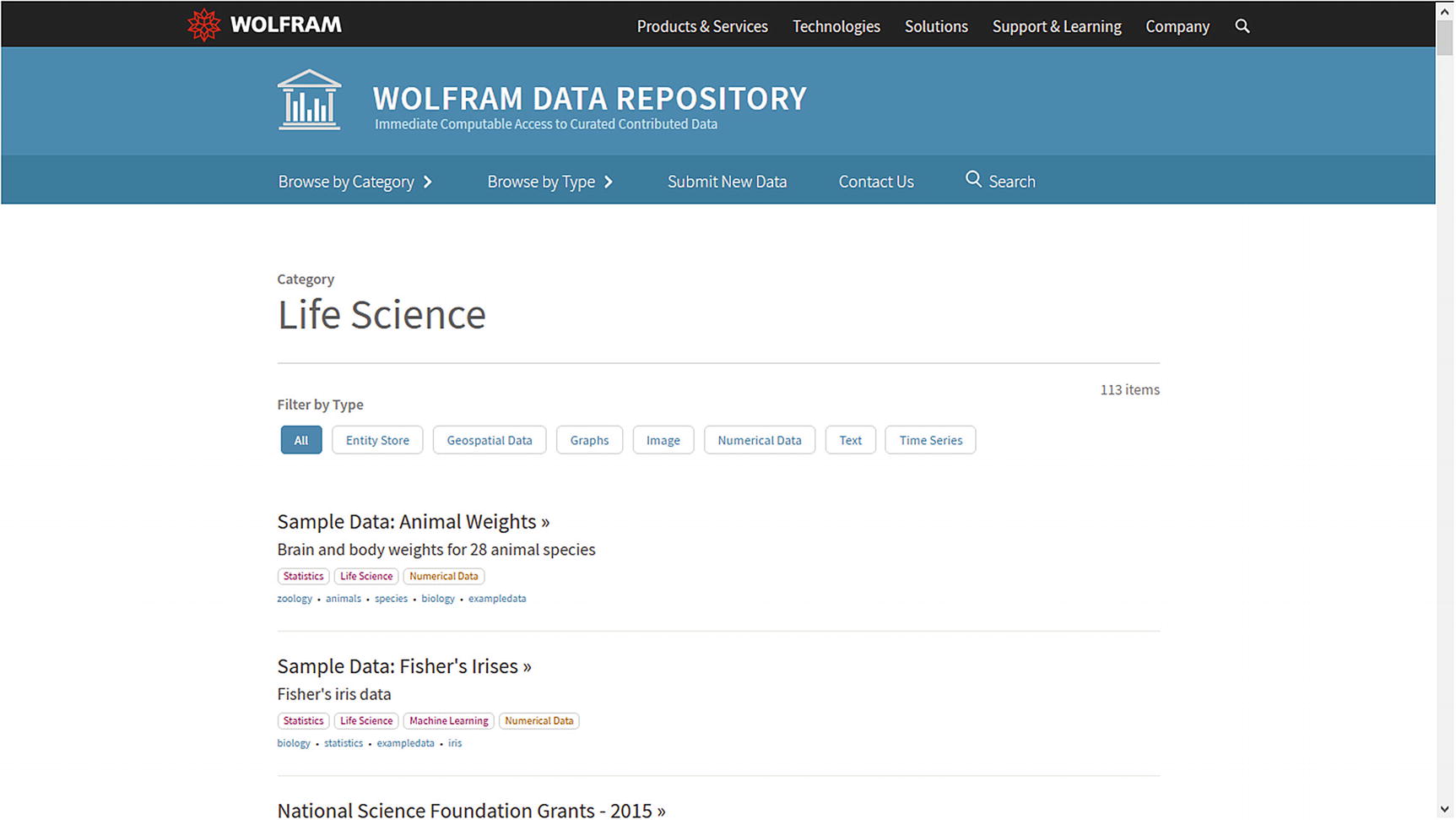
Life Science category of the Wolfram Data Repository

Note

The same process is for when we navigate by data type.

Selecting a Category

Each category shows the title, the number of elements contained in that category, and the option to filter the contents of that category by the type of data. Regarding the content, each sample data type is displayed with its title, a small description of the data it contains, and the different tags associated with that sample data. For example, the image shows Fisher's Irises known dataset. Once we select a sample dataset, it will take us to the site where the relevant information about that dataset is contained, as shown in Figure 7-4, where the Fisher's Irises dataset is selected.
../images/500903_1_En_7_Chapter/500903_1_En_7_Fig4_HTML.jpg
Figure 7-4

Fisher’s Irises dataset

When a sample dataset is selected, a brief description of the dataset is shown as well as the different calculations that can be made and different formats to download the data or the notebook. Besides this, it also includes relevant information such as the bibliographic citation, data resource history, and data source. In certain cases, the data can either be downloaded for different types of formats such as comma-separated value (CSV), tab-separated value (TSV), JavaScript object notation (JSON), and others. Before starting to download data from the Wolfram Data Repository, it is necessary to have a Wolfram ID. This ID is an account that gives us access to the content of the Wolfram Data Repository in addition to other benefits such as the Wolfram One and Wolfram Alpha. To log in from Mathematica, head to the menu in Help ➤ Sign in, and a window will appear like the one in Figure 7-5.
../images/500903_1_En_7_Chapter/500903_1_En_7_Fig5_HTML.jpg
Figure 7-5

Wolfram Cloud sign-in prompt

In the new window, you will enter your email and password to be able to access from Mathematica the contents of the Wolfram Data Repository.

Extracting Data from the Wolfram Data Repository

Let’s start by looking at the information and properties of the Fisher’s dataset; for this we must retrieve the information through a ResourceObject. With ResourceObject (Figure 7-6) we can now view the different properties of the published data by clicking the plus icon. Detailed information about the data will display, such as sample name, type, version, size of the data, and many more.
In[2]:= ResourceObject["Sample Data: Fisher's Irises"]
Out[2]=
../images/500903_1_En_7_Chapter/500903_1_En_7_Fig6_HTML.jpg
Figure 7-6

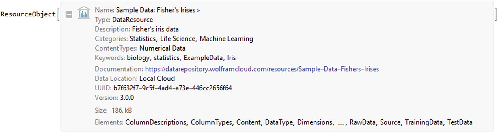
ResourceObject of the Fisher´s Irises

If we wanted to look to the properties of the resource object, enter the following code. This will give us a list of properties that can be accessed and that are related to the data sample.
In[3]:= ResourceObject["Sample Data: Fisher's Irises"]["Properties"]
Out[3]= {AllVersions,AutoUpdate,Categories,ContentElementLocations,ContentElements,ContentSize,ContentTypes,ContributorInformation,DefaultContentElement,Description,Details,Documentation,DocumentationLink,DOI,DownloadedVersion,ExampleNotebook,ExampleNotebookObject,Format,InformationElements,Keywords,LatestUpdate,Name,Originator,Properties,ReleaseDate,RepositoryLocation,ResourceLocations,ResourceType,SeeAlso,ShortName,SourceMetadata,UUID,Version,VersionInformation,VersionsAvailable,WolframLanguageVersionRequired}
Knowing already the list of properties related to information, we can now download from Mathematica the exercise notebook of the data sample.
In[4]:= ResourceObject["Sample Data: Fisher's Irises"]["ExampleNotebook"]
Out[4]= NotebookObject[Sample-Data-Fishers-Irises_examples.nb]
Once you finish evaluating the code, it will automatically open the new notebook. If we want to operate the notebook from the Cloud, we can type NotebookObject. This will give us back a Cloud, like object that is associated with a hyperlink.
In[5]:= ResourceObject["Sample Data: Fisher's Irises"]["ExampleNotebookObject"]
Out[5]= CloudObject[https://www.wolframcloud.com/obj/5e59b79e-d95e-4f6f-a7c8-f1276ba17be2]
If we press the link of the new notebook, it will open the internet browser and show us that it is in the Wolfram Cloud. Figure 7-7 shows this.
../images/500903_1_En_7_Chapter/500903_1_En_7_Fig7_HTML.jpg
Figure 7-7

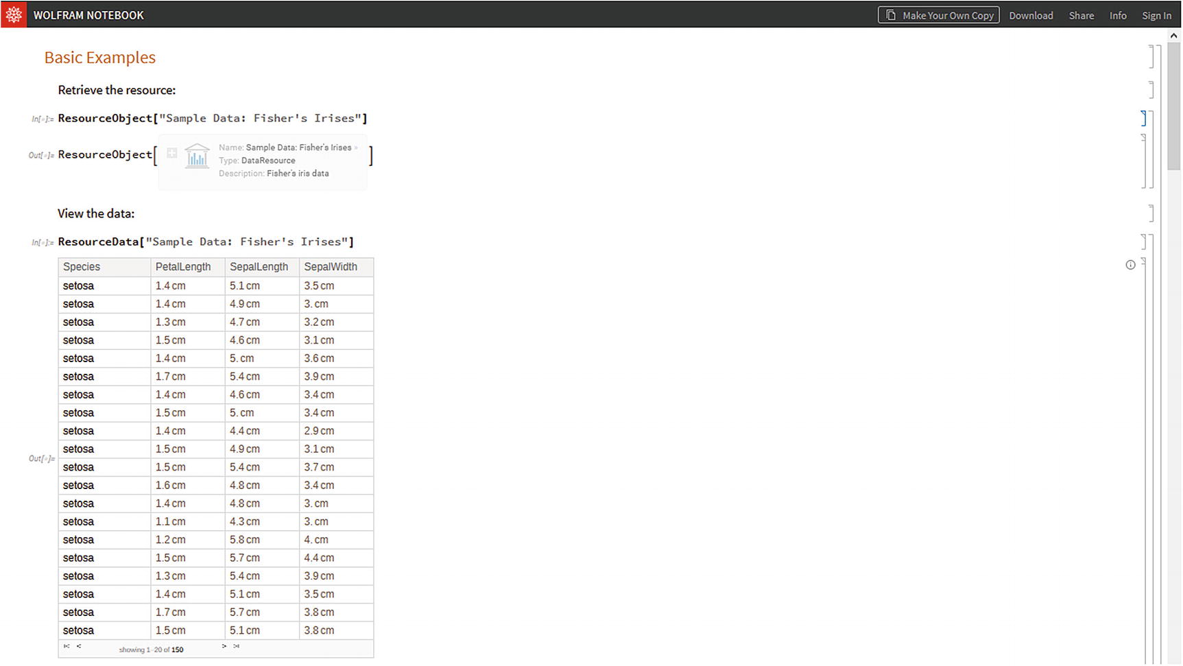
Fisher´s Irises data sample, open from the Wolfram Cloud

To access from Mathematica to the original sample data site, we enter Documentation, which will give us a URL object that you can enter to the site by clicking the double chevron icon.
In[6]:= ResourceObject["Sample Data: Fisher's Irises"]["Documentation"]
Out[6]= URL[https://datarepository.wolframcloud.com/resources/Sample-Data-Fishers-Irises]

Accessing Data Inside Mathematica

The same initiative is applied to downloading the data using the ResourceData to the object resource. With ResourceData we access the contents of the specified resource; in this case, it is the Fisher’s Irises data sample (Figure 7-8).
In[7]:= ResourceData[ResourceObject["Sample Data: Fisher's Irises"]]
Out[7]=
../images/500903_1_En_7_Chapter/500903_1_En_7_Fig8_HTML.jpg
Figure 7-8

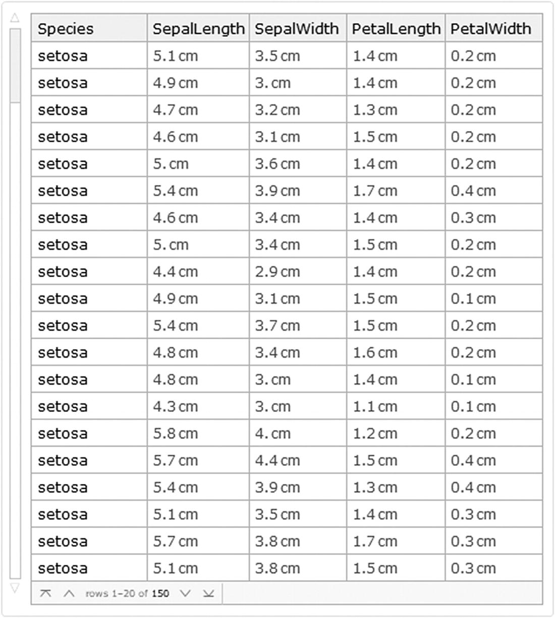
Fisher’s Irises dataset object

As shown in Figure 7-8, the object that is returned is a ResourceData to use with a head of Dataset. Performing a visual inspection of the data sample, we observe that it is a dataset of 150 values, which contains five columns: Species, SepalLength, SepalWidth, PetalLength, and PetalWidth. If we pay attention, we can see how the values of the columns SepalLength, SepalWidth, PetalLength, and PetalWidth are quantities. Moving further down the entire dataset, we find that the species are divided into three categories: setosa, versicolor, and virginica. If we want to access the information related to the dataset, we must do it through the resource object and retrieve it through a ResourceData form, as shown.
In[8]:= ResourceObject["Sample Data: Fisher's Irises"]["ContentElements"]
Out[8]={ColumnDescriptions,ColumnTypes,Content,DataType,Dimensions,ObservationCount,RawData,Source,TrainingData,TestData}
With the ContentElements property, we are accessing the elements of the data sample, which are the ones that appear within the resource object. ContentElements shows us the information associated with the sample data, such as column information, data source, training data, test data, etc.—not to be confused with the properties of the resource object created, as it is not the same since you can construct a resource object for another associated name. To retrieve the information from the ContentElements, we must do it with ResourceData. This command will give us access to the contents of the data sample—in this case, the Fisher’s Irises. Now let’s get the data type of the columns.
In[9]:= ResourceData[ResourceObject["Sample Data: Fisher's Irises"],"ColumnTypes"]
Out[9]= {Numeric,Numeric,Numeric,Numeric,Categorical}
The second argument of the ResourceData command is the element we are looking for. Running the aforementioned code shows us that there are four data types, three numeric and one categorical. Using a pure function, we can obtain information in a single expression. If we add the Column command, it is possible to have a better view of the information.
In[10]:= Column[ResourceData[ResourceObject["Sample Data: Fisher's Irises"],#]&/@{"ColumnDescriptions","Dimensions","Source"}]
Out[10]= {Sepal length in cm.,Sepal width in cm.,Petal length in cm.,Petal width in cm.,Species of iris}
{150,4}
Fisher,R.A. "The use of multiple measurements in taxonomic problems" Annual Eugenics, 7, Part II, 179-188 (1936); also in "Contributions to Mathematical Statistics" (John Wiley, NY, 1950).

This way we get to know the type of information in the columns ,such as dimensions, which are 150 rows per 4 columns and the data source.

Data Observation

In this part we will see how to observe data inside a dataset. We will use the Iris dataset, which has been extracted from the Wolfram Data Repository. Let’s start by naming the data sample Fisher; this variable will contain the dataset with quantities included.
In[11]:= Fisher=ResourceData[ResourceObject["Sample Data: Fisher's Irises"]];
If we look at the dataset, we will notice that the numbers have their units and magnitude. Having the dataset, we can perform endless processes, such as grouping the content by the category variable that is the type of species. It is necessary to emphasize that I will access the dataset contained in the Fisher’s variable. Let's look at the type of data that contains each column grouped by species (Figure 7-9).
In[12]:= Fisher[GroupBy["Species"]]
Out[12]=
../images/500903_1_En_7_Chapter/500903_1_En_7_Fig9_HTML.jpg
Figure 7-9

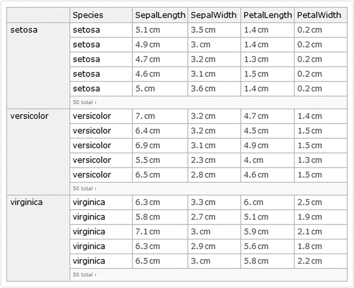
Iris data grouped by species

Let us notice how the data is divided into three categories: setosa, versicolor, and virginica. If we pay attention to detail, we will notice that each of these categories contains a number 50 at the end of the Species column of each category. This means that there are 50 more rows in addition to those shown, making a total of 50 for each category that is 150 rows in total, which matches the number of 150 we review the dimensions of the sample data. In the meantime, if we click one of the categories, it will show us the columns for that category alone, as shown in the Figure 7-10. The same happens if we select the specific column within a category—it will show only that column for that category; try it to see what happens. There is also the possibility to click any column, and this will show us only the chosen column but for the three categories. By this I mean that if, for example, we choose SepalLength, we will see the contents of that column for the three species, as shown in Figure 7-10
../images/500903_1_En_7_Chapter/500903_1_En_7_Fig10_HTML.jpg
Figure 7-10

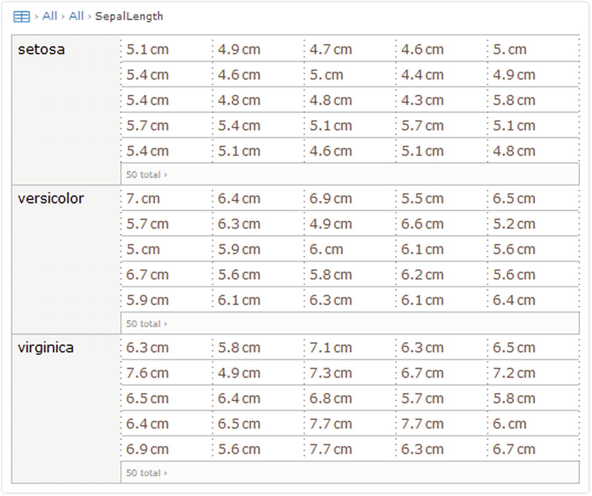
SepalLength column selected

It is possible to group by species and choose only the columns that contain numeric values. This helps if, for example, we wanted to make a visual inspection of the dataset (Figure 7-11).
In[13]:= Query[GroupBy[Key["Species"]→KeyTake[{"SepalLength","SepalWidth","PetalLength","PetalWidth"}]]][Fisher]
Out[13]=
../images/500903_1_En_7_Chapter/500903_1_En_7_Fig11_HTML.jpg
Figure 7-11

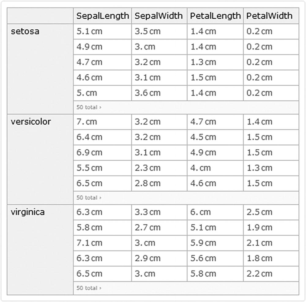
Dataset with the species column suppressed

What happens in the latter code is that we use the Key command to access the keys of the species column. Once these keys are accessed, we write a transformation rule so that each extracted key is assigned the associations extracted (KeyTake) from columns (SepalLength, SepalWidth, PetalLength, PetalWidth), then grouped and applied to Fisher’s dataset.

If we wanted to count the data elements in the Fisher’s dataset, we can add an ID column as a label (Figure 7-12) to list the data it contains. To achieve this, first we create an association with keys and values that go from 1 to the length of the dataset. Then this instruction is applied to the dataset object Fisher’s, which adds the ID’s as labels for the rows.
In[14]:= Query[AssociationThread[Range[Length@#]→Range[Length@#]]][Fisher]&[Fisher]
Out[14]=
../images/500903_1_En_7_Chapter/500903_1_En_7_Fig12_HTML.jpg
Figure 7-12

ID's added to the Fisher´s dataset

If we drag down the bar, we see that the counter reaches 150 elements.

In case you don’t want to add an enumerated column to count the elements, we can use the Counts command (Figure 7-13).
In[15]:= Fisher[Counts,"Species"]
Out[15]=
../images/500903_1_En_7_Chapter/500903_1_En_7_Fig13_HTML.jpg
Figure 7-13

Counted elements on the dataset

This results in 50 data belonging to setosa, versicolor, and virginica. If we add them up, we get 150. You can also use the Query command, Query[Counts, "Species"][Fisher].

Now let’s see how to get the average of the three categories for each column. It would be possible if we knew the average of SepalLength, SepalWidth, PetalLength, and PetalWidth for the species, setosa, versicolor, and virginica, as exhibited in Figure 7-15.
In[16]:= Query[GroupBy[Key["Species"]→KeyTake[{"SepalLength","SepalWidth","PetalLength","PetalWidth"}]],Mean][Fisher]
Out[16]=
../images/500903_1_En_7_Chapter/500903_1_En_7_Fig14_HTML.jpg
Figure 7-14

Mean for the four columns, divided by species

But, if we want to get the average of the columns for all categories, one way to get it would be by applying Mean as a query to the number of columns in the entire dataset (Figure 7-15).
In[17]:= Query[Mean][Fisher[[All,2;;5]]]
Out[17]=
../images/500903_1_En_7_Chapter/500903_1_En_7_Fig15_HTML.jpg
Figure 7-15

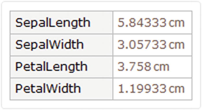
Average values for the four columns of all species

Note

The Mean command works with the quantities and returns the average to use as a quantity.

Descriptive Statistics

In this part we will see how to perform descriptive statistic of the Irises data and computations inside the format of the dataset as well as how to create custom grid formats. Let’s get some descriptive statistics about this dataset. Let’s create a function that would be called Stats. Let us start by building the function that will calculate the maximum, minimum, mean, median, first, and third quartile.
In[18]:= Stats[data_]:=
{
{#[{"Max:",Max@data}]},
{#[{"Min:",Min@data}]},
{#[{"Mean:",Mean@data}]},
{#[{"Median:",Median@data}]},
{#[{"1st quartile:",Quantile[data,0.25]}]},
{#[{"3rd quartile:",Quantile[data,0.75]}]}
}&[Row]
Now apply the created function to each of the columns. This is to get overall statistics for SepalLength, SepalWidth, PetalLength, and PetalWidth (Figure 7-16).
In[19]:= {{#1,#2,#3,#4},{Fisher[Stats,#1],Fisher[Stats,#2],Fisher[Stats,#3],Fisher[Stats,#4]}}&["SepalLength","SepalWidth","PetalLength","PetalWidth"]//Grid
Out[19]=
../images/500903_1_En_7_Chapter/500903_1_En_7_Fig16_HTML.jpg
Figure 7-16

Function Stats applied to each column

This also can be displayed in a compact form in a tab format with TabView (Figure 7-17).
In[20]:= TabView[{#1→Fisher[Stats,#1],#2→Fisher[Stats,#2],#3→Fisher[Stats,#3],#4→Fisher[Stats,#4]},ControlPlacement→Left]&["SepalLength","SepalWidth","PetalLength","PetalWidth"]
Out[20]=
../images/500903_1_En_7_Chapter/500903_1_En_7_Fig17_HTML.jpg
Figure 7-17

Tabview format

With TabView, we create three tabs with the names of each column, where it shows the values maximum, minimum, average, median, first, and third quartile; the columns are SepalLength, SepalWidth, PetalLength, and PetalWidth.

Table and Grid Formats

An alternative is to create a table for each species. In this way, we will create a better presentation of the data and thus be able to read it properly. We extract the data by applying the Nest command. With this command, we can specify the number of times a command or function will be applied; in this case, we will apply it twice.
In[21]:= Short[Values[Nest[Normal,Fisher,2]]]
{SLall,SWall,PLall,PWall}=%[[All,#]]&/@{2,3,4,5};
Out[21]//Short= {{setosa,5.1cm,3.5cm,1.4cm,0.2cm},{setosa,4.9cm,3.cm,1.4cm,0.2cm},<<146>>,{virginica,6.2cm,3.4cm,5.4cm,2.3cm},{virginica,5.9cm,3.cm,5.1cm,1.8cm}}
Having the values of all species separated by columns, we will proceed to create a list instead of a function, where the statistics will be displayed according to each column, adding calculations such as variance, standard deviation, skewness, and kurtosis. Then we will assign the calculations in the variable DescriptiveStats.
In[22]:= {Max[#],Min[#],Median[#],Mean[#],Variance[#],StandardDeviation[#],Skewness[#],Kurtosis[#],Quantile[#,0.25],Quantile[#,.75]}&/@{SLall,SWall,PLall,PWall};
DescriptiveStats=%;
A table (Figure 7-18) can be created with these calculations and adding the rows and column headings.
In[23]:=
TableHeads={
Style["Sepal Length",#1,ColorData["HTML"]["Maroon"],#2,#3],
Style["Sepal Width",#1,ColorData["HTML"]["YellowGreen"],#2,#3],
Style["Petal Length",#1,ColorData["HTML"]["SteelBlue"],#2,#3],
Style["Petal Width",#1,ColorData["HTML"]["Orange"],#2,#3]
}&["Title",Italic,20];
TableRows={
Style["Max",#1,#2],Style["Min",#1,#2],
Style["Median",#1,#2],Style["Mean",#1,#2],Style["Variance",#1,#2],
Style["Standard Deviation",#1,#2],
Style["Skewness",#1,#2],
Style["Kurtosis",#1,#2],
Style["1st quartile",#1,#2],
Style["3rd quartile",#1,#2]
}&["Text",Italic];
TableForm[DescriptiveStats,TableHeadings→{TableHeads,TableRows}]
Out[23]=
../images/500903_1_En_7_Chapter/500903_1_En_7_Fig18_HTML.jpg
Figure 7-18

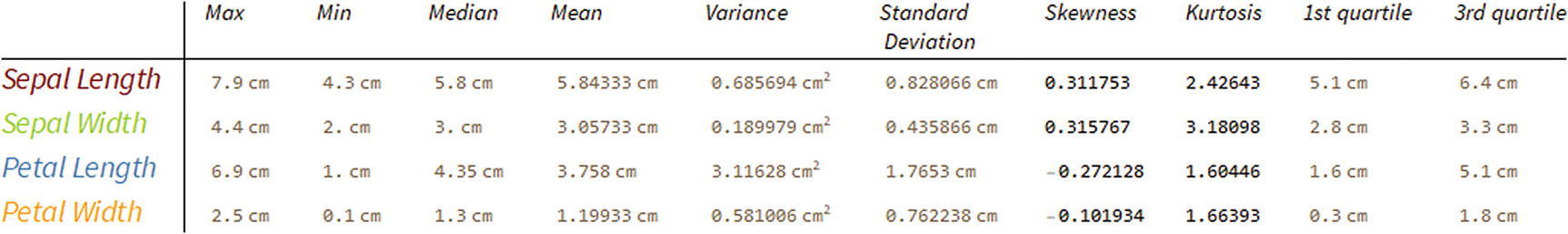
Table showing descriptive statistics by the four features

Note that the statistics are calculated with their units, with the exception of skewness and kurtosis, since by definition they are dimensionless. However, we can create a better structure from Grid because it is possible to add dividers like a spreadsheet format. To do this, we will add the TableRows to the data and then apply a transpose so that each calculated statistic is with its respective name. Subsequently we will add the column titles.
In[24]:= Transpose[Prepend[DescriptiveStats,TableRows]];
{" ",Style["Sepal Length",#1,ColorData["HTML"]["Maroon"],#2,#3],Style["Sepal Width",#1,ColorData["HTML"]["YellowGreen"],#2,#3],Style["Petal Length",#1,ColorData["HTML"]["SteelBlue"],#2,#3],
Style["Petal Width",#1,ColorData["HTML"]["Orange"],#2,#3]
}&["Title",Italic,20];
NewTable=Prepend[%%,%];
We proceed to create the table in the form of a spreadsheet (Figure 7-19).
In[25]:= Grid[NewTable,
ItemSize→{{None, Scaled[0.11], Scaled[0.11],Scaled[0.11]}},Background→{{LightGray},None},Dividers→{{False},{1,2,3,4,5,6,7,8,9,10,11→True,-2→Blue}},Alignment→Center]
Out[25]:=
../images/500903_1_En_7_Chapter/500903_1_En_7_Fig19_HTML.jpg
Figure 7-19

Grid view of the descriptive statistics

If we want to build the table for each species, we will have to first separate the dataset by species with the Cases command. We use Cases since it gives us the freedom to work with patterns. First write the code to extract the raw data, and instead of using Short, we will use Shallow to suppress the 150 values.
In[26]:= Shallow[Values[Nest[Normal,Fisher,2]],1]
Out[26]//Shallow= {<<150>>}
We will create the table for the versicolor species and proceed to extract the values for versicolor and storethe values of the columns in the variables SLVersi, SWVersi, PLVersi, and PWVersi.
In[27]:= Shallow[Cases[%,{"versicolor",__}],1]
{SLVersi,SWVersi,PLVersi,PWVersi}=%[[All,#]]&/@{2,3,4,5};
Out[27]//Shallow= {<<50>>}
We do the same construction as before for the calculation of statistics. But instead of the white space, we add the name versicolor to distinguish that the table belongs to the versicolor specie.
In[28]:= TableRows;
{Max[#],Min[#],Median[#],Mean[#],Variance[#],StandardDeviation[#],Skewness[#],Kurtosis[#],Quantile[#,0.25],Quantile[#,.75]}&/@{SLVersi,SWVersi,PLVersi,PWVersi};
DescriptiveStats2=Prepend[%,%%];
Transpose[DescriptiveStats2];
{
Style["Versicolor","Text",Red,Italic,20],Style["Sepal Length",#1,ColorData["HTML"]["Maroon"],#2,#3],
Style["Sepal Width",#1,ColorData["HTML"]["YellowGreen"],#2,#3],
Style["Petal Length",#1,ColorData["HTML"]["SteelBlue"],#2,#3],
Style["Petal Width",#1,ColorData["HTML"]["Orange"],#2,#3]
}&["Title",Italic,20];
NewTable2=Prepend[%%,%];
Now we build the table (Figure 7-20) for the species versicolor.
In[29]:= Grid[NewTable2,ItemSize→{{None, Scaled[0.11], Scaled[0.11],Scaled[0.11]}},Background→{{LightGray},None},Dividers→{{False},{1,2,3,4,5,6,7,8,9,10,11→True,-2→Blue}},Alignment→Center]
Out[29]=
../images/500903_1_En_7_Chapter/500903_1_En_7_Fig20_HTML.jpg
Figure 7-20

Descriptive stats for the versicolor specie

We have only done this for the species of versicolor; if required the same process will be performed for each species. For example, if choose Cases with the other species, we would change the text to the corresponding specie.

Dataset Visualization

Having viewed the capabilities of the Wolfram Language to perform descriptive statistics within dataset, statistical charts can be implemented inside the dataset format, as we will see in this fragment.

We can have a better perspective from graphs, we will use the dataset format (Figure 7-21) to display the graphs by their species.
In[30]:= Fisher[GroupBy["Species"],DistributionChart[#,PlotTheme→"Classic",PlotLabel→"PetalLength cm", GridLines→Automatic]&,"]&,"PetalLength"]
Out[30]=
../images/500903_1_En_7_Chapter/500903_1_En_7_Fig21_HTML.jpg
Figure 7-21

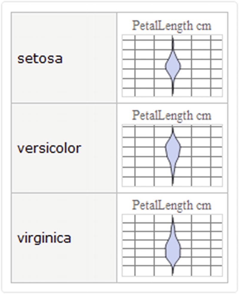
Distribution chart plot

We can perform the same process but for the box whiskers plot (Figure 7-22), but choose another column.
In[31]:= Fisher[GroupBy["Species"],BoxWhiskerChart[#,"Outliers",PlotTheme→"Detailed",ChartLabels→Placed[{"SepalLength cm"},Above],BarOrigin→Right,ChartStyle→Blue]&,"SepalLength"]
Out[31]=
../images/500903_1_En_7_Chapter/500903_1_En_7_Fig22_HTML.jpg
Figure 7-22

Box whiskers plot

If the specie is clicked, it will amplify the graph (Figure 7-23).
../images/500903_1_En_7_Chapter/500903_1_En_7_Fig23_HTML.jpg
Figure 7-23

Box whiskers plot for virginica specie

The same applies for histograms. When the graph is very large, it appears suppressed within the dataset, but we can still select it, as shown in Figure 7-24.
In[32]:=Fisher[GroupBy["Species"],
 Labeled[Histogram[#,
    ColorFunction → (Hue[3/5, 2/3, #] &)], {Rotate["Frequency",
     90 Degree], "SepalWidth cm"}, {Left, Bottom}] &, "SepalWidth"]
Out[32]=
../images/500903_1_En_7_Chapter/500903_1_En_7_Fig24_HTML.jpg
Figure 7-24

Histogram plot for versicolor
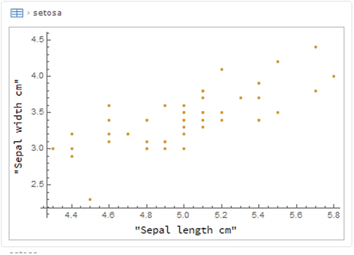
Here we show the 3D scatter plots for each species (Figure 7-25) for sepal length (x) vs sepal width (y).
In[33]:=Fisher[GroupBy["Species"],
 Labeled[ListPlot[{#, #}], {Rotate["Sepal width cm", 90 Degree], "Sepal length cm"}, {Left, Bottom}] &, {"SepalLength","SepalWidth"}]
Out[33]=
../images/500903_1_En_7_Chapter/500903_1_En_7_Fig25_HTML.jpg
Figure 7-25

2D scatter plot

To return to the full dataset, click the dataset icon as with any other.

Data Outside Dataset Format

The truth is that there is also the possibility to extract the data crudely, as follows. We’ll do this to have better data handling. We will use the Short command since the list is quite long.
In[34]:= Short[ResourceData[ResourceObject["Sample Data: Fisher's Irises"],"RawData"]]
Out[34]//Short= {<<1>>}
With the data already extracted, we can get the values with the Values function and convert them to normal expressions.
In[35]:= Short[Normal[Values[%]]]
Out[35]//Short= {{setosa,5.1cm,3.5cm,1.4cm,0.2cm},{setosa,4.9cm,3.cm,1.4cm,0.2cm},<<146>>,{virginica,6.2cm,3.4cm,5.4cm,2.3cm},{virginica,5.9cm,3.cm,5.1cm,1.8cm}}
With the help of MapAt, we can extract the magnitudes of the quantities. The MapAt command gives us the freedom to choose where we want to apply the Quantity function. We choose to apply it to all rows with All, but only from column 2 to 4, which is where the quantities are located.
In[36]:= Short[Iris=MapAt[QuantityMagnitude,%,{All,2;;5}]]
Out[36]//Short= {{setosa,5.1,3.5,1.4,0.2},<<148>>,{virginica,5.9,3.,5.1,1.8}}

It's worth asking a question here: Why do we remove the units if calculations can be made with them? We extract the magnitudes for all quantities because they have the same order of magnitude (cm), so each calculation will be in the same units, except if we made conversions or transformations to the data.

2D and 3D Plots

On the other hand, it is easier to manipulate lists with Wolfram Language. Having the data in the form of lists, we will now proceed to plot the three columns in a box plot and a distribution graph (Figure 7-26). We will only choose the three columns of the data.
In[37]:= Row[
{BoxWhiskerChart[{Iris[[All,#1]],Iris[[All,#2]],Iris[[All,#3]],Iris[[All,#4]]},"Outliers",PlotRange→Automatic,FrameTicks→True,ChartStyle→"SandyTerrain",PlotLabel→"All Species",GridLines→Automatic,ChartLegends→Placed[{"SepalLength","SepalWidth","PetalLength","PetalWidth"},Bottom],ImageSize→Small],DistributionChart[{Iris[[All,#1]],Iris[[All,#2]],Iris[[All,#3]],Iris[[All,#4]]},PlotRange→Automatic,FrameTicks→True,ChartStyle→"SouthwestColors",PlotLabel→"All Species",ChartLegends→Placed[{"SepalLength","SepalWidth","PetalLength","PetalWidth"},Bottom],PlotTheme→"Detailed",GridLines→Automatic,ImageSize→Small]
}]&[2,3,4,5]
Out[37]=
../images/500903_1_En_7_Chapter/500903_1_En_7_Fig26_HTML.jpg
Figure 7-26

Box whiskers plot and distribution chart for all species

To improve this, let us graph for each species. We will use Cases to separate the list with their respective species (Figure 7-27).
In[38]:= Short[Setosa=Cases[Iris,{"setosa",__}]]
Short[Versi=Cases[Iris,{"versicolor",__}]]
Short[Virgin=Cases[Iris,{"virginica",__}]]
Out[38]//Short= {{setosa,5.1,3.5,1.4,0.2},<<48>>,{setosa,5.,3.3,1.4,0.2}}
Out[38]//Short= {{versicolor,7.,3.2,4.7,1.4},<<48>>,{versicolor,5.7,2.8,4.1,1.3}}
Out[38]//Short= {{virginica,6.3,3.3,6.,2.5},<<48>>,{virginica,5.9,3.,5.1,1.8}}
In[39]:= Column@{
BoxWhiskerChart[{Setosa[[All,#1]],Setosa[[All,#2]],Setosa[[All,#3]],Setosa[[All,#4]]},"Outliers",PlotRange→Automatic,FrameTicks→True,ChartStyle→"Rainbow",PlotLabel→"Setosa",ChartLegends→Placed[{"SepalLength","SepalWidth","PetalLength","PetalWidth"},Bottom],GridLines→Automatic],BoxWhiskerChart[{Versi[[All,#1]],Versi[[All,#2]],Versi[[All,#3]],Versi[[All,#4]]},"Outliers",PlotRange→Automatic,FrameTicks→True,ChartStyle→"Rainbow",PlotLabel→"Versicolor",ChartLegends→Placed[{"SepalLength","SepalWidth","PetalLength","PetalWidth"},Bottom],GridLines→Automatic],BoxWhiskerChart[{Virgin[[All,#1]],Virgin[[All,#2]],Virgin[[All,#3]],Virgin[[All,#4]]},"Outliers",PlotRange→Automatic,FrameTicks→True,ChartStyle→"Rainbow",PlotLabel→"Virginica",ChartLegends→Placed[{"SepalLength","SepalWidth","PetalLength","PetalWidth"},Bottom],GridLines→Automatic]
}&[2,3,4,5]
Out[39]=
../images/500903_1_En_7_Chapter/500903_1_En_7_Fig27_HTML.jpg
Figure 7-27

Box whiskers plot for every specie with the four features

In addition, we can join the scatter plots of sepal width vs sepal length for all species (Figure 7-28).
In[40]:= ListPlot[{Setosa[[All,{2,3}]],Versi[[All,{2,3}]],Virgin[[All,{2,3}]]},FrameTicks→All,Frame→True,AspectRatio→1,PlotStyle→{Blue,Red,Green},FrameLabel→{"Sepal length cm","Sepal width cm"},PlotLegends→{"Setosa","Versicolor","Virginica"}]
Out[40]=
../images/500903_1_En_7_Chapter/500903_1_En_7_Fig28_HTML.jpg
Figure 7-28

2D scatter plot for all species of the first two features

Or we can make a 3D scatter plot with three features (Figure 7-29).
In[41]:= ListPointPlot3D[{Setosa[[All,{2,3,4}]],Versi[[All,{2,3,4}]],Virgin[[All,{2,3,4}]]},Ticks→All,AspectRatio→1,PlotStyle→{Blue,Red,Green},AxesLabel→{"Sepal length cm","Sepal width cm","Petal Length cm"},PlotLegends→{"Setosa","Versicolor","Virginica"},PlotTheme→"Detailed",ViewPoint→{0, -3, 3}]
Out[41]=
../images/500903_1_En_7_Chapter/500903_1_En_7_Fig29_HTML.jpg
Figure 7-29

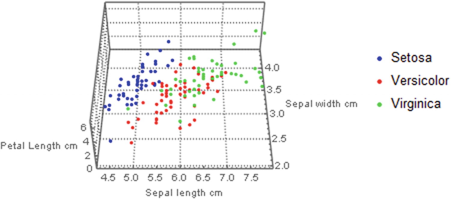
3D scatter plot of three features for every species

Now, when we have finished working with the resource object, we need to delete it so that the local cache of the resource is properly removed.
In[42]:=Clear[Fisher]
DeleteObject[ResourceObject["Sample Data: Fisher's Irises"]]
..................Content has been hidden....................

You can't read the all page of ebook, please click here login for view all page.
Reset
3.143.23.176