13
Measuring Performance and Big O Algorithm Analysis
For most small programs, performance isn’t all that important. We might spend an hour writing a script to automate a task that needs only a few seconds to run. Even if it takes longer, the program will probably finish by the time we’ve returned to our desk with a cup of coffee.
Sometimes it’s prudent to invest time in learning how to make a script faster. But we can’t know if our changes improve a program’s speed until we know how to measure program speed. This is where Python’s timeit and cProfile modules come in. These modules not only measure how fast code runs, but also create a profile of which parts of the code are already fast and which parts we could improve.
In addition to measuring program speed, in this chapter you’ll also learn how to measure the theoretical increases in runtime as the data for your program grows. In computer science, we call this big O notation. Software developers without traditional computer science backgrounds might sometimes feel they have gaps in their knowledge. But although a computer science education is fulfilling, it’s not always directly relevant to software development. I joke (but only half so) that big O notation makes up about 80 percent of the usefulness of my degree. This chapter provides an introduction to this practical topic.
The timeit Module
“Premature optimization is the root of all evil” is a common saying in software development. (It’s often attributed to computer scientist Donald Knuth, who attributes it to computer scientist Tony Hoare. Tony Hoare, in turn, attributes it to Donald Knuth.) Premature optimization, or optimizing before knowing what needs to be optimized, often manifests itself when programmers try to use clever tricks to save memory or write faster code. For example, one of these tricks is using the XOR algorithm to swap two integer values without using a third, temporary variable:
>>> a, b = 42, 101  # Set up the two variables.
>>> print(a, b)
42 101
>>> # A series of ^ XOR operations will end up swapping their values:
>>> a = a ^ b
>>> b = a ^ b
>>> a = a ^ b
>>> print(a, b)  # The values are now swapped.
101 42
Unless you’re unfamiliar with the XOR algorithm (which uses the ^ bitwise operator), this code looks cryptic. The problem with using clever programming tricks is that they can produce complicated, unreadable code. Recall that one of the Zen of Python tenets is readability counts.
Even worse, your clever trick might turn out not to be so clever. You can’t just assume a crafty trick is faster or that the old code it’s replacing was even all that slow to begin with. The only way to find out is by measuring and comparing the runtime: the amount of time it takes to run a program or piece of code. Keep in mind that increasing the runtime means the program is slowing down: the program is taking more time to do the same amount of work. (We also sometimes use the term runtime to refer to the period during which the program is running. This error happened at runtime means the error happened while the program was running as opposed to when the program was being compiled into bytecode.)
The Python standard library’s timeit module can measure the runtime speed of a small snippet of code by running it thousands or millions of times, letting you determine an average runtime. The timeit module also temporarily disables the automatic garbage collector to ensure more consistent runtimes. If you want to test multiple lines, you can pass a multiline code string or separate the code lines using semicolons:
>>> import timeit
>>> timeit.timeit('a, b = 42, 101; a = a ^ b; b = a ^ b; a = a ^ b')
0.1307766629999998
>>> timeit.timeit("""a, b = 42, 101
... a = a ^ b
... b = a ^ b
... a = a ^ b""")
0.13515726800000039
On my computer, the XOR algorithm takes roughly one-tenth of a second to run this code. Is this fast? Let’s compare it to some integer swapping code that uses a third temporary variable:
>>> import timeit
>>> timeit.timeit('a, b = 42, 101; temp = a; a = b; b = temp')
0.027540389999998638
That’s a surprise! Not only is using a third temporary variable more readable, but it’s also twice as fast! The clever XOR trick might save a few bytes of memory but at the expense of speed and code readability. Sacrificing code readability to reduce a few bytes of memory usage or nanoseconds of runtime isn’t worthwhile.
Better still, you can swap two variables using the multiple assignment trick, also called iterable unpacking, which also runs in a small amount of time:
>>> timeit.timeit('a, b = 42, 101; a, b = b, a')
0.024489236000007963
Not only is this the most readable code, it’s also the quickest. We know this not because we assumed it, but because we objectively measured it.
The timeit.timeit() function can also take a second string argument of setup code. The setup code runs only once before running the first string’s code. You can also change the default number of trials by passing an integer for the number keyword argument. For example, the following test measures how quickly Python’s random module can generate 10,000,000 random numbers from 1 to 100. (On my machine, it takes about 10 seconds.)
>>> timeit.timeit('random.randint(1, 100)', 'import random', number=10000000)
10.020913950999784
By default, the code in the string you pass to timeit.timeit() won’t be able to access the variables and the functions in the rest of the program:
>>> import timeit
>>> spam = 'hello'  # We define the spam variable.
>>> timeit.timeit('print(spam)', number=1)  # We measure printing spam.
Traceback (most recent call last):
  File "<stdin>", line 1, in <module>
  File "C:UsersAlAppDataLocalProgramsPythonPython37lib	imeit.py", line 232, in timeit
    return Timer(stmt, setup, timer, globals).timeit(number)
  File "C:UsersAlAppDataLocalProgramsPythonPython37lib	imeit.py", line 176, in timeit
    timing = self.inner(it, self.timer)
  File "<timeit-src>", line 6, in inner
NameError: name 'spam' is not defined
To fix this, pass the function the return value of globals() for the globals keyword argument:
>>> timeit.timeit('print(spam)', number=1, globals=globals())
hello
0.000994909999462834
A good rule for writing your code is to first make it work and then make it fast. Only once you have a working program should you focus on making it more efficient.
The cProfile Profiler
Although the timeit module is useful for measuring small code snippets, the cProfile module is more effective for analyzing entire functions or programs. Profiling analyzes your program’s speed, memory usage, and other aspects systematically. The cProfile module is Python’s profiler, or software that can measure a program’s runtime as well as build a profile of runtimes for the program’s individual function calls. This information provides substantially more granular measurements of your code.
To use the cProfile profiler, pass a string of the code you want to measure to cProfile.run(). Let’s look at how cProfiler measures and reports the execution of a short function that sums all the numbers from 1 to 1,000,000:
import time, cProfile
def addUpNumbers():
    total = 0
    for i in range(1, 1000001):
        total += i

cProfile.run('addUpNumbers()')
When you run this program, the output will look something like this:
         4 function calls in 0.064 seconds

   Ordered by: standard name

   ncalls  tottime  percall  cumtime  percall filename:lineno(function)
        1    0.000    0.000    0.064    0.064 <string>:1(<module>)
        1    0.064    0.064    0.064    0.064 test1.py:2(addUpNumbers)
        1    0.000    0.000    0.064    0.064 {built-in method builtins.exec}
        1    0.000    0.000    0.000    0.000 {method 'disable' of '_lsprof.Profiler' objects}
Each line represents a different function and the amount of time spent in that function. The columns in cProfile.run()’s output are:
- ncalls The number of calls made to the function
- tottime The total time spent in the function, excluding time in subfunctions
- percall The total time divided by the number of calls
- cumtime The cumulative time spent in the function and all subfunctions
- percall The cumulative time divided by the number of calls
- filename:lineno(function) The file the function is in and at which line number
For example, download the rsaCipher.py and al_sweigart_pubkey.txt files from https://nostarch.com/crackingcodes/. This RSA Cipher program was featured in Cracking Codes with Python (No Starch Press, 2018). Enter the following into the interactive shell to profile the encryptAndWriteToFile() function as it encrypts a 300,000-character message created by the 'abc' * 100000 expression:
>>> import cProfile, rsaCipher
>>> cProfile.run("rsaCipher.encryptAndWriteToFile('encrypted_file.txt', 'al_sweigart_pubkey.txt', 'abc'*100000)")
         11749 function calls in 28.900 seconds

   Ordered by: standard name

   ncalls  tottime  percall  cumtime  percall filename:lineno(function)
        1    0.001    0.001   28.900   28.900 <string>:1(<module>)
        2    0.000    0.000    0.000    0.000 _bootlocale.py:11(getpreferredencoding)
--snip--
        1    0.017    0.017   28.900   28.900 rsaCipher.py:104(encryptAndWriteToFile)
        1    0.248    0.248    0.249    0.249 rsaCipher.py:36(getBlocksFromText)
        1    0.006    0.006   28.873   28.873 rsaCipher.py:70(encryptMessage)
        1    0.000    0.000    0.000    0.000 rsaCipher.py:94(readKeyFile)
--snip--
     2347    0.000    0.000    0.000    0.000 {built-in method builtins.len}
     2344    0.000    0.000    0.000    0.000 {built-in method builtins.min}
     2344   28.617    0.012   28.617    0.012 {built-in method builtins.pow}
        2    0.001    0.000    0.001    0.000 {built-in method io.open}
     4688    0.001    0.000    0.001    0.000 {method 'append' of 'list' objects}
--snip--
You can see that the code passed to cProfile.run() took 28.9 seconds to complete. Pay attention to the functions with the highest total times; in this case, Python’s built-in pow() function takes up 28.617 seconds. That’s nearly the entire code’s runtime! We can’t change this code (it’s part of Python), but perhaps we could change our code to rely on it less.
This isn’t possible in this case, because rsaCipher.py is already fairly optimized. Even so, profiling this code has provided us insight that pow() is the main bottleneck. So there’s little sense in trying to improve, say, the readKeyFile() function (which takes so little time to run that cProfile reports its runtime as 0).
This idea is captured by Amdahl’s Law, a formula that calculates how much the overall program speeds up given an improvement to one of its components. The formula is speed-up of whole task = 1 / ((1 – p) + (p / s)) where s is the speed-up made to a component and p is the portion of that component of the overall program. So if you double the speed of a component that makes up 90 percent of the program’s total runtime, you’ll get 1 / ((1 – 0.9) + (0.9 / 2)) = 1.818, or an 82 percent speed-up of the overall program. This is better than, say, tripling the speed of a component that only makes up 25 percent of the total runtime, which would only be a 1 / ((1 – 0.25) + (0.25 / 2)) = 1.143, or 14 percent overall speed-up. You don’t need to memorize the formula. Just remember that doubling the speed of your code’s slow or lengthy parts is more productive than doubling the speed of an already quick or short part. This is common sense: a 10 percent price discount on an expensive house is better than a 10 percent discount on a cheap pair of shoes.
Big O Algorithm Analysis
Big O is a form of algorithm analysis that describes how code will scale. It classifies the code into one of several orders that describes, in general terms, how much longer the code’s runtime will take as the amount of work it has to do increases. Python developer Ned Batchelder describes big O as an analysis of “how code slows as data grows,” which is also the title of his informative PyCon 2018 talk, which is available at https://youtu.be/duvZ-2UK0fc/.
Let’s consider the following scenario. Say you have a certain amount of work that takes an hour to complete. If the workload doubles, how long would it take then? You might be tempted to think it takes twice as long, but actually, the answer depends on the kind of work that’s being done.
If it takes an hour to read a short book, it will take more or less two hours to read two short books. But if you can alphabetize 500 books in an hour, alphabetizing 1,000 books will most likely take longer than two hours, because you have to find the correct place for each book in a much larger collection of books. On the other hand, if you’re just checking whether or not a bookshelf is empty, it doesn’t matter if there are 0, 10, or 1,000 books on the shelf. One glance and you’ll immediately know the answer. The runtime remains roughly constant no matter how many books there are. Although some people might be faster or slower at reading or alphabetizing books, these general trends remain the same.
The big O of the algorithm describes these trends. An algorithm can run on a fast or slow computer, but we can still use big O to describe how well an algorithm performs in general, regardless of the actual hardware executing the algorithm. Big O doesn’t use specific units, such as seconds or CPU cycles, to describe an algorithm’s runtime, because these would vary between different computers or programming languages.
Big O Orders
Big O notation commonly defines the following orders. These range from the lower orders, which describe code that, as the amount of data grows, slows down the least, to the higher orders, which describe code that slows down the most:
- O(1), Constant Time (the lowest order)
- O(log n), Logarithmic Time
- O(n), Linear Time
- O(n log n), N-Log-N Time
- O(n2), Polynomial Time
- O(2n), Exponential Time
- O(n!), Factorial Time (the highest order)
Notice that big O uses the following notation: a capital O, followed by a pair of parentheses containing a description of the order. The capital O represents order or on the order of. The n represents the size of the input data the code will work on. We pronounce O(n) as “big oh of n” or “big oh n.”
You don’t need to understand the precise mathematic meanings of words like logarithmic or polynomial to use big O notation. I’ll describe each of these orders in detail in the next section, but here’s an oversimplified explanation of them:
- O(1) and O(log n) algorithms are fast.
- O(n) and O(n log n) algorithms aren’t bad.
- O(n2), O(2n), and O(n!) algorithms are slow.
Certainly, you could find counterexamples, but these descriptions are good rules in general. There are more big O orders than the ones listed here, but these are the most common. Let’s look at the kinds of tasks that each of these orders describes.
A Bookshelf Metaphor for Big O Orders
In the following big O order examples, I’ll continue using the bookshelf metaphor. The n refers to the number of books on the bookshelf, and the big O ordering describes how the various tasks take longer as the number of books increases.
O(1), Constant Time
Finding out “Is the bookshelf empty?” is a constant time operation. It doesn’t matter how many books are on the shelf; one glance tells us whether or not the bookshelf is empty. The number of books can vary, but the runtime remains constant, because as soon as we see one book on the shelf, we can stop looking. The n value is irrelevant to the speed of the task, which is why there is no n in O(1). You might also see constant time written as O(c).
O(log n), Logarithmic
Logarithms are the inverse of exponentiation: the exponent 24, or 2 × 2 × 2 × 2, equals 16, whereas the logarithm log2(16) (pronounced “log base 2 of 16”) equals 4. In programming, we often assume base 2 to be the logarithm base, which is why we write O(log n) instead of O(log2 n).
Searching for a book on an alphabetized bookshelf is a logarithmic time operation. To find one book, you can check the book in the middle of the shelf. If that is the book you’re searching for, you’re done. Otherwise, you can determine whether the book you’re searching for comes before or after this middle book. By doing so, you’ve effectively reduced the range of books you need to search in half. You can repeat this process again, checking the middle book in the half that you expect to find it. We call this the binary search algorithm, and there’s an example of it in “Big O Analysis Examples” later in this chapter.
The number of times you can split a set of n books in half is log2 n. On a shelf of 16 books, it will take at most four steps to find the right one. Because each step reduces the number of books you need to search by one half, a bookshelf with double the number of books takes just one more step to search. If there were 4.2 billion books on the alphabetized bookshelf, it would still only take 32 steps to find a particular book.
Log n algorithms usually involve a divide and conquer step, which selects half of the n input to work on and then another half from that half, and so on. Log n operations scale nicely: the workload n can double in size, but the runtime increases by only one step.
O(n), Linear Time
Reading all the books on a bookshelf is a linear time operation. If the books are roughly the same length and you double the number of books on the shelf, it will take roughly double the amount of time to read all the books. The runtime increases in proportion to the number of books n.
O(n log n), N-Log-N Time
Sorting a set of books into alphabetical order is an n-log-n time operation. This order is the runtime of O(n) and O(log n) multiplied together. You can think of a O(n log n) task as a O(log n) task that must be performed n times. Here’s a casual description of why.
Start with a stack of books to alphabetize and an empty bookshelf. Follow the steps for a binary search algorithm, as detailed in “O(log n), Logarithmic” on page 232, to find where a single book belongs on the shelf. This is an O(log n) operation. With n books to alphabetize, and each book taking log n steps to alphabetize, it takes n × log n, or n log n, steps to alphabetize the entire set of books. Given twice as many books, it takes a bit more than twice as long to alphabetize all of them, so n log n algorithms scale fairly well.
In fact, all of the efficient general sorting algorithms are O(n log n): merge sort, quicksort, heapsort, and Timsort. (Timsort, invented by Tim Peters, is the algorithm that Python’s sort() method uses.)
O(n2), Polynomial Time
Checking for duplicate books on an unsorted bookshelf is a polynomial time operation. If there are 100 books, you could start with the first book and compare it with the 99 other books to see whether they’re the same. Then you take the second book and check whether it’s the same as any of the 99 other books. Checking for a duplicate of a single book is 99 steps (we’ll round this up to 100, which is our n in this example). We have to do this 100 times, once for each book. So the number of steps to check for any duplicate books on the bookshelf is roughly n × n, or n2. (This approximation to n2 still holds even if we were clever enough not to repeat comparisons.)
The runtime increases by the increase in books squared. Checking 100 books for duplicates is 100 × 100, or 10,000 steps. But checking twice that amount, 200 books, is 200 × 200, or 40,000 steps: four times as much work.
In my experience writing code in the real world, I’ve found the most common use of big O analysis is to avoid accidentally writing an O(n2) algorithm when an O(n log n) or O(n) algorithm exists. The O(n2) order is when algorithms dramatically slow down, so recognizing your code as O(n2) or higher should give you pause. Perhaps there’s a different algorithm that can solve the problem faster. In these cases, taking a data structure and algorithms (DSA) course, whether at a university or online, can be helpful.
We also call O(n2) quadratic time. Algorithms could have O(n3), or cubic time, which is slower than O(n2); O(n4), or quartic time, which is slower than O(n3); or other polynomial time complexities.
O(2n), Exponential Time
Taking photos of the shelf with every possible combination of books on it is an exponential time operation. Think of it this way: each book on the shelf can either in be included in the photo or not included. Figure 13-1 shows every combination where n is 1, 2, or 3. If n is 1, there are two possible photos: with the book and without. If n is 2, there are four possible photos: both books on the shelf, both books off, the first on and second off, and the second on and first off. When you add a third book, you’ve once again doubled the amount of work you have to do: you need to do every subset of two books that includes the third book (four photos) and every subset of two books that excludes the third book (another four photos, for 23 or eight photos). Each additional book doubles the workload. For n books, the number of photos you need to take (that is, the amount of work you need to do) is 2n.
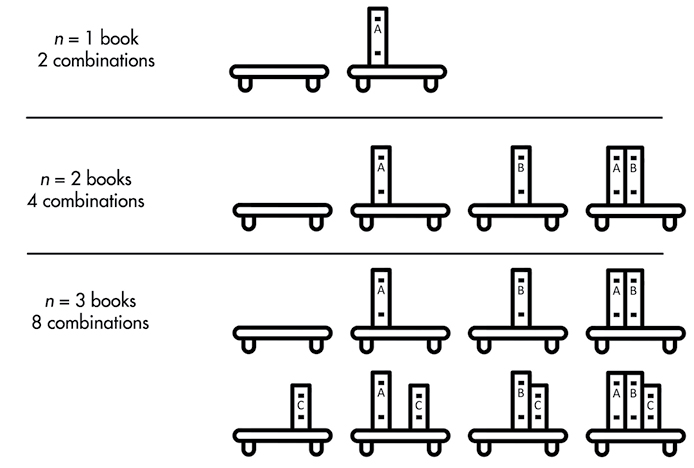
Figure 13-1: Every combination of books on a bookshelf for one, two, or three books
The runtime for exponential tasks increases very quickly. Six books require 26 or 32 photos, but 32 books would include 232 or more than 4.2 billion photos. O(2n), O(3n), O(4n), and so on are different orders ut all have exponential time complexity.
O(n!), Factorial Time
Taking a photo of the books on the shelf in every conceivable order is a factorial time operation. We call every possible order the permutation of n books. This results in n!, or n factorial, orderings. The factorial of a number is the multiplication product of all positive integers up to the number. For example, 3! is 3 × 2 × 1, or 6. Figure 13-2 shows every possible permutation of three books.

Figure 13-2: All 3! (that is, 6) permutations of three books on a bookshelf
To calculate this yourself, think about how you would come up with every permutation of n books. You have n possible choices for the first book; then n – 1 possible choices for the second book (that is, every book except the one you picked for the first book); then n – 2 possible choices for the third book; and so on. With 6 books, 6! results in 6 × 5 × 4 × 3 × 2 × 1, or 720 photos. Adding just one more book makes this 7!, or 5,040 photos needed. Even for small n values, factorial time algorithms quickly become impossible to complete in a reasonable amount of time. If you had 20 books and could arrange them and take a photo every second, it would still take longer than the universe has existed to get through every possible permutation.
One well-known O(n!) problem is the traveling salesperson conundrum. A salesperson must visit n cities and wants to calculate the distance travelled for all n! possible orders in which they could visit them. From these calculations, they could determine the order that involves the shortest travel distance. In a region with many cities, this task proves impossible to complete in a timely way. Fortunately, optimized algorithms can find a short (but not guaranteed to be the shortest) route much faster than O(n!).
Big O Measures the Worst-Case Scenario
Big O specifically measures the worst-case scenario for any task. For example, finding a particular book on an unorganized bookshelf requires you to start from one end and scan the books until you find it. You might get lucky, and the book you’re looking for might be the first book you check. But you might be unlucky; it could be the last book you check or not on the bookshelf at all. So in a best-case scenario, it wouldn’t matter if there were billions of books you had to search through, because you’ll immediately find the one you’re looking for. But that optimism isn’t useful for algorithm analysis. Big O describes what happens in the unlucky case: if you have n books on the shelf, you’ll have to check all n books. In this example, the runtime increases at the same rate as the number of books.
Some programmers also use big Omega notation, which describes the best-case scenario for an algorithm. For example, a Ω(n) algorithm performs at linear efficiency at its best. In the worst case, it might perform slower. Some algorithms encounter especially lucky cases where no work has to be done, such as finding driving directions to a destination when you’re already at the destination.
Big Theta notation describes algorithms that have the same best- and worst-case order. For example, Θ(n) describes an algorithm that has linear efficiency at best and at worst, which is to say, it’s an O(n) and Ω(n) algorithm. These notations aren’t used in software engineering as often as big O, but you should still be aware of their existence.
It isn’t uncommon for people to talk about the “big O of the average case” when they mean big Theta, or “big O of the best case” when they mean big Omega. This is an oxymoron; big O specifically refers to an algorithm’s worst-case runtime. But even though their wording is technically incorrect, you can understand their meaning irregardless.
Determining the Big O Order of Your Code
To determine the big O order for a piece of code, we must do four tasks: identify what the n is, count the steps in the code, drop the lower orders, and drop the coefficients.
For example, let’s find the big O of the following readingList() function:
def readingList(books):
    print('Here are the books I will read:')
    numberOfBooks = 0
    for book in books:
        print(book)
        numberOfBooks += 1
    print(numberOfBooks, 'books total.')
Recall that the n represents the size of the input data that the code works on. In functions, the n is almost always based on a parameter. The readingList() function’s only parameter is books, so the size of books seems like a good candidate for n, because the larger books is, the longer the function takes to run.
Next, let’s count the steps in this code. What counts as a step is somewhat vague, but a line of code is a good rule to follow. Loops will have as many steps as the number of iterations multiplied by the lines of code in the loop. To see what I mean, here are the counts for the code inside the readingList() function:
def readingList(books):
    print('Here are the books I will read:')  # 1 step
    numberOfBooks = 0                         # 1 step
    for book in books:                        # n * steps in the loop
        print(book)                           # 1 step
        numberOfBooks += 1                    # 1 step
    print(numberOfBooks, 'books total.')      # 1 step
We’ll treat each line of code as one step except for the for loop. This line executes once for each item in books, and because the size of books is our n, we say that this executes n steps. Not only that, but it executes all the steps inside the loop n times. Because there are two steps inside the loop, the total is 2 × n steps. We could describe our steps like this:
def readingList(books):
    print('Here are the books I will read:')  # 1 step
    numberOfBooks = 0                         # 1 step
    for book in books:                        # n * 2 steps
        print(book)                           # (already counted)
        numberOfBooks += 1                    # (already counted)
    print(numberOfBooks, 'books total.')      # 1 step
Now when we compute the total number of steps, we get 1 + 1 + (n × 2) + 1. We can rewrite this expression more simply as 2n + 3.
Big O doesn’t intend to describe specifics; it’s a general indicator. Therefore, we drop the lower orders from our count. The orders in 2n + 3 are linear (2n) and constant (3). If we keep only the largest of these orders, we’re left with 2n.
Next, we drop the coefficients from the order. In 2n, the coefficient is 2. After dropping it, we’re left with n. This gives us the final big O of the readingList() function: O(n), or linear time complexity.
This order should make sense if you think about it. There are several steps in our function, but in general, if the books list increases tenfold in size, the runtime increases about tenfold as well. Increasing books from 10 books to 100 books moves the algorithm from 1 + 1 + (2 × 10) + 1, or 23 steps, to 1 + 1 + (2 × 100) + 1, or 203 steps. The number 203 is roughly 10 times 23, so the runtime increases proportionally with the increase to n.
Why Lower Orders and Coefficients Don’t Matter
We drop the lower orders from our step count because they become less significant as n grows in size. If we increased the books list in the previous readingList() function from 10 to 10,000,000,000 (10 billion), the number of steps would increase from 23 to 20,000,000,003. With a large enough n, those extra three steps matter very little.
When the amount of data increases, a large coefficient for a smaller order won’t make a difference compared to the higher orders. At a certain size n, the higher orders will always be slower than the lower orders. For example, let’s say we have quadraticExample(), which is O(n2) and has 3n2 steps. We also have linearExample(), which is O(n) and has 1,000n steps. It doesn’t matter that the 1,000 coefficient is larger than the 3 coefficient; as n increases, eventually an O(n2) quadratic operation will become slower than an O(n) linear operation. The actual code doesn’t matter, but we can think of it as something like this:
def quadraticExample(someData):  # n is the size of someData
    for i in someData:           # n steps
        for j in someData:       # n steps
            print('Something')   # 1 step
            print('Something')   # 1 step
            print('Something')   # 1 step

def linearExample(someData):     # n is the size of someData
    for i in someData:           # n steps
        for k in range(1000):    # 1 * 1000 steps
            print('Something')   # (Already counted)
The linearExample() function has a large coefficient (1,000) compared to the coefficient (3) of quadraticExample(). If the size of the input n is 10, the O(n2) function appears faster with only 300 steps compared to the O(n) function with 10,000 steps.
But big O notation is chiefly concerned with the algorithm’s performance as the workload scales up. When n reaches the size of 334 or greater, the quadraticExample() function will always be slower than the linearExample() function. Even if linearExample() were 1,000,000n steps, the quadraticExample() function would still become slower once n reached 333,334. At some point, an O(n2) operation always becomes slower than an O(n) or lower operation. To see how, look at the big O graph shown in Figure 13-3. This graph features all the major big O notation orders. The x-axis is n, the size of the data, and the y-axis is the runtime needed to carry out the operation.
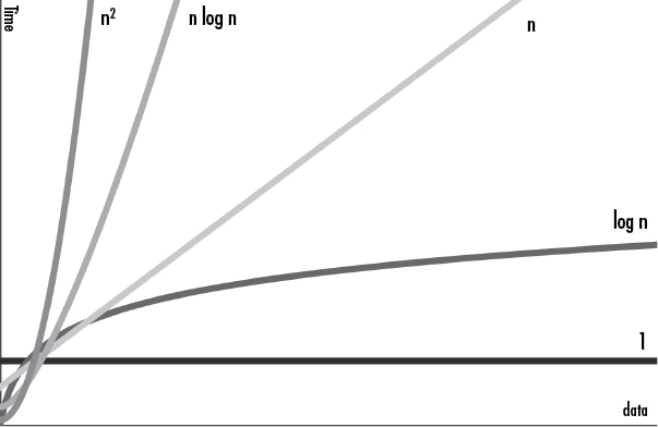
Figure 13-3: The graph of the big O orders
As you can see, the runtime of the higher orders grows at a faster rate than that of the lower orders. Although the lower orders could have large coefficients that make them temporarily larger than the higher orders, the higher orders eventually outpace them.
Big O Analysis Examples
Let’s determine the big O orders of some example functions. In these examples, we’ll use a parameter named books that is a list of strings of book titles.
The countBookPoints() function calculates a score based on the number of books in the books list. Most books are worth one point, and books by a certain author are worth two points:
def countBookPoints(books):
    points = 0          # 1 step
    for book in books:  # n * steps in the loop
        points += 1     # 1 step

    for book in books:                # n * steps in the loop
        if 'by Al Sweigart' in book:  # 1 step
            points += 1               # 1 step
    return points                     # 1 step
The number of steps comes to 1 + (n × 1) + (n × 2) + 1, which becomes 3n + 2 after combining the like terms. Once we drop the lower orders and coefficients, this becomes O(n), or linear complexity, no matter if we loop through books once, twice, or a billion times.
So far, all examples that used a single loop have had linear complexity, but notice that these loops iterated n times. As you’ll see in the next example, a loop in your code alone doesn’t imply linear complexity, although a loop that iterates over your data does.
This iLoveBooks() function prints “I LOVE BOOKS!!!” and “BOOKS ARE GREAT!!!” 10 times:
def iLoveBooks(books):
    for i in range(10):              # 10 * steps in the loop
        print('I LOVE BOOKS!!!')     # 1 step
        print('BOOKS ARE GREAT!!!')  # 1 step
This function has a for loop, but it doesn’t loop over the books list, and it performs 20 steps no matter what the size of books is. We can rewrite this as 20(1). After dropping the 20 coefficient, we are left with O(1), or constant time complexity. This makes sense; the function takes the same amount of time to run, no matter what n, the size of the books list, is.
Next, we have a cheerForFavoriteBook() function that searches through the books list to look for a favorite book:
def cheerForFavoriteBook(books, favorite):
    for book in books:                            # n * steps in the loop
        print(book)                               # 1 step
        if book == favorite:                      # 1 step
            for i in range(100):                  # 100 * steps in the loop
                print('THIS IS A GREAT BOOK!!!')  # 1 step
The for book loop iterates over the books list, which requires n steps multiplied by the steps inside the loop. This loop includes a nested for i loop, which iterates 100 times. This means the for book loop runs 102 × n, or 102n steps. After dropping the coefficient, we find that cheerForFavoriteBook() is still just an O(n) linear operation. This 102 coefficient might seem rather large to just ignore, but consider this: if favorite never appears in the books list, this function would only run 1n steps. The impact of coefficients can vary so wildly that they aren’t very meaningful.
Next, the findDuplicateBooks() function searches through the books list (a linear operation) once for each book (another linear operation):
def findDuplicateBooks(books):
    for i in range(books):  # n steps
        for j in range(i + 1, books):          # n steps
            if books[i] == books[j]:           # 1 step
                print('Duplicate:', books[i])  # 1 step
The for i loop iterates over the entire books list, performing the steps inside the loop n times. The for j loop also iterates over a portion of the books list, although because we drop coefficients, this also counts as a linear time operation. This means the for i loop performs n × n operations—that is, n2. This makes findDuplicateBooks() an O(n2) polynomial time operation.
Nested loops alone don’t imply a polynomial operation, but nested loops where both loops iterate n times do. These result in n2 steps, implying an O(n2) operation.
Let’s look at a challenging example. The binary search algorithm mentioned earlier works by searching the middle of a sorted list (we’ll call it the haystack) for an item (we’ll call it the needle). If we don’t find the needle there, we’ll proceed to search the previous or latter half of the haystack, depending on which half we expect to find the needle in. We’ll repeat this process, searching smaller and smaller halves until either we find the needle or we conclude it isn’t in the haystack. Note that binary search only works if the items in the haystack are in sorted order.
def binarySearch(needle, haystack):
    if not len(haystack):                        # 1 step
        return None                              # 1 step
    startIndex = 0                               # 1 step
    endIndex = len(haystack) - 1                 # 1 step

    haystack.sort()                              # ??? steps

    while start <= end:  # ??? steps
        midIndex = (startIndex + endIndex) // 2  # 1 step
        if haystack[midIndex] == needle:         # 1 step
            # Found the needle.
            return midIndex                      # 1 step
        elif needle < haystack[midIndex]:        # 1 step
            # Search the previous half.
            endIndex = midIndex - 1              # 1 step
        elif needle > haystack[mid]:             # 1 step
            # Search the latter half.
            startIndex = midIndex + 1            # 1 step
Two of the lines in binarySearch() aren’t easy to count. The haystack.sort() method call’s big O order depends on the code inside Python’s sort() method. This code isn’t very easy to find, but you can look up its big O order on the internet to learn that it’s O(n log n). (All general sorting functions are, at best, O(n log n).) We’ll cover the big O order of several common Python functions and methods in “The Big O Order of Common Function Calls” later in this chapter.
The while loop isn’t as straightforward to analyze as the for loops we’ve seen. We must understand the binary search algorithm to determine how many iterations this loop has. Before the loop, the startIndex and endIndex cover the entire range of haystack, and midIndex is set to the midpoint of this range. On each iteration of the while loop, one of two things happens. If haystack[midIndex] == needle, we know we’ve found the needle, and the function returns the index of the needle in haystack. If needle < haystack[midIndex] or needle > haystack[midIndex], the range covered by startIndex and endIndexis halved, either by adjusting startIndex or adjusting endIndex. The number of times we can divide any list of size n in half is log2(n). (Unfortunately, this is simply a mathematical fact that you’d be expected to know.) Thus, the while loop has a big O order of O(log n).
But because the O(n log n) order of the haystack.sort() line is higher than O(log n), we drop the lower O(log n) order, and the big O order of the entirebinarySearch() function becomes O(n log n). If we can guarantee that binarySearch() will only ever be called with a sorted list for haystack, we can remove the haystack.sort() line and make binarySearch() an O(log n) function. This technically improves the function’s efficiency but doesn’t make the overall program more efficient, because it just moves the required sorting work to some other part of the program. Most binary search implementations leave out the sorting step and therefore the binary search algorithm is said to have O(log n) logarithmic complexity.
The Big O Order of Common Function Calls
Your code’s big O analysis must consider the big O order of any functions it calls. If you wrote the function, you can just analyze your own code. But to find the big O order of Python’s built-in functions and methods, you’ll have to consult lists like the following.
This list contains the big O orders of some common Python operations for sequence types, such as strings, tuples, and lists:
s[i] reading and s[i] = value assignmentO(1) operations.s.append(value)An O(1) operation.s.insert(i, value)An O(n) operation. Inserting values into a sequence (especially at the front) requires shifting all the items at indexes aboveiup by one place in the sequence.s.remove(value)An O(n) operation. Removing values from a sequence (especially at the front) requires shifting all the items at indexes aboveIdown by one place in the sequence.s.reverse()An O(n) operation, because every item in the sequence must be rearranged.s.sort()An O(n log n) operation, because Python’s sorting algorithm is O(n log n).value in sAn O(n) operation, because every item must be checked.for value in s:An O(n) operation.len(s)An O(1) operation, because Python keeps track of how many items are in a sequence so it doesn’t need to recount them when passed tolen().
This list contains the big O orders of some common Python operations for mapping types, such as dictionaries, sets, and frozensets:
m[key] reading and m[key] = value assignmentO(1) operations.m.add(value)An O(1) operation.value in mAn O(1) operation for dictionaries, which is much faster than usinginwith sequences.for key in m:An O(n) operation.len(m)An O(1) operation, because Python keeps track of how many items are in a mapping, so it doesn’t need to recount them when passed tolen().
Although a list generally has to search through its items from start to finish, dictionaries use the key to calculate the address, and the time needed to look up the key’s value remains constant. This calculation is called a hashing algorithm, and the address is called a hash. Hashing is beyond the scope of this book, but it’s the reason so many of the mapping operations are O(1) constant time. Sets also use hashing, because sets are essentially dictionaries with keys only instead of key-value pairs.
But keep in mind that converting a list to a set is an O(n) operation, so you don’t achieve any benefit by converting a list to a set and then accessing the items in the set.
Analyzing Big O at a Glance
Once you’ve become familiar with performing big O analysis, you usually won’t need to run through each of the steps. After a while you’ll be able to just look for some telltale features in the code to quickly determine the big O order.
Keeping in mind that n is the size of the data the code operates on, here are some general rules you can use:
- If the code doesn’t access any of the data, it’s O(1).
- If the code loops over the data, it’s O(n).
- If the code has two nested loops that each iterate over the data, it’s O(n2).
- Function calls don’t count as one step but rather the total steps of the code inside the function. See “Big O Order of Common Function Calls” on page 242.
- If the code has a divide and conquer step that repeatedly halves the data, it’s O(log n).
- If the code has a divide and conquer step that is done once per item in the data, it’s an O(n log n).
- If the code goes through every possible combination of values in the n data, it’s O(2n), or some other exponential order.
- If the code goes through every possible permutation (that is, ordering) of the values in the data, it’s O(n!).
- If the code involves sorting the data, it will be at least O(n log n).
These rules are good starting points. But they’re no substitute for actual big O analysis. Keep in mind that big O order isn’t the final judgment on whether code is slow, fast, or efficient. Consider the following waitAnHour() function:
import time
def waitAnHour():
    time.sleep(3600)
Technically, the waitAnHour() function is O(1) constant time. We think of constant time code as fast, yet its runtime is one hour! Does that make this code inefficient? No: it’s hard to see how you could have programmed a waitAnHour() function that runs faster than, well, one hour.
Big O isn’t a replacement for profiling your code. The point of big O notation is to give you insights as to how the code will perform under increasing amounts of input data.
Big O Doesn’t Matter When n Is Small, and n Is Usually Small
Armed with the knowledge of big O notation, you might be eager to analyze every piece of code you write. Before you start using this tool to hammer every nail in sight, keep in mind that big O notation is most useful when there is a large amount of data to process. In real-world cases, the amount of data is usually small.
In those situations, coming up with elaborate, sophisticated algorithms with lower big O orders might not be worth the effort. Go programming language designer Rob Pike has five rules about programming, one of which is: “Fancy algorithms are slow when ‘n’ is small, and ‘n’ is usually small.” Most software developers won’t be dealing with massive data centers or complex calculations but rather more mundane programs. In these circumstances, running your code under a profiler will yield more concrete information about the code’s performance than big O analysis.
Summary
The Python standard library comes with two modules for profiling: timeit and cProfile. The timeit.timeit() function is useful for running small snippets of code to compare the speed difference between them. The cProfile.run() function compiles a detailed report on larger functions and can point out any bottlenecks.
It’s important to measure the performance of your code rather than make assumptions about it. Clever tricks to speed up your program might actually slow it down. Or you might spend lots of time optimizing what turns out to be an insignificant aspect of your program. Amdahl’s Law captures this mathematically. The formula describes how a speed-up to one component affects the speed-up of the overall program.
Big O is the most widely used practical concept in computer science for programmers. It requires a bit of math to understand, but the underlying concept of figuring out how code slows as data grows can describe algorithms without requiring significant number crunching.
There are seven common orders of big O notation: O(1), or constant time, describes code that doesn’t change as the size of the data n grows; O(log n), or logarithmic time, describes code that increases by one step as the n data doubles in size; O(n), or linear time, describes code that slows in proportion to the n data’s growth; O(n log n), or n-log-n time, describes code that is a bit slower than O(n), and many sorting algorithms have this order.
The higher orders are slower, because their runtime grows much faster than the size of their input data: O(n2), or polynomial time, describes code whose runtime increases by the square of the n input; O(2n), or exponential time, and O(n!), or factorial time, orders are uncommon, but come up when combinations or permutations are involved, respectively.
Keep in mind that although big O is a helpful analysis tool, it isn’t a substitute for running your code under a profiler to find out where any bottlenecks are. But an awareness of big O notation and how code slows as data grows can help you avoid writing code that is orders slower than it needs to be.