
Chapter 5
Letting the Data Speak with Unsupervised Learning
Introduction
The supervised learning discussed in Chapter 3 typically requires a hypothesis and a neatly matching set of inputs and outputs. The semi-supervised learning covered in Chapter 4 relaxes some assumptions about data. The unsupervised learning (UL) discussed here and in the rest of this book does away with hypotheses, instead allowing the data to drive the analytical process.
In econometrics, a researcher dreams up a question to ask the data. The resulting question may be subjective, incomplete, outright irrelevant, or even severely biased by the researcher's own prejudice. Unsupervised learning eliminates the trickling of the researcher's personal opinions and beliefs into the analysis. Instead of waiting for the researcher's question, unsupervised learning tells the researcher what the data know. Specifically, unsupervised methods explain to the researcher the major trends in the data, the main factors driving observed behavior and the like, all at the stroke of a key on a computer keyboard.
UL is taking the industry by storm. Traditional disciplines like risk management can be improved by switching to a fast hypothesis-less environment, trusting the data to speak for themselves.
UL also comes with computational benefits: unsupervised techniques deliver results of complex mathematical analyses in a flash, all with existing computing power. The implementation of UL can reach most areas, saving corporations millions of dollars in the process. For example, one application that is waiting to benefit from unsupervised learning is modern risk management, where at present most financial decisions are made with at least a few days of risk horizon. Such a view ignores short-term risk events. The classic 10-day value at risk (VAR), a standard for banks, for example, misses many short-term risk events that end up costing financial institutions a pretty penny. The duration of the traditional risk measures was chosen as a balance between the application and the computational complexity. Many traditional models require extensive Monte-Carlo simulations that may take a very long time. This chapter and the following chapters in this book discuss the details of implementation of the fast hypothesis-less paradigm in Big Data Science.
The core unsupervised learning techniques have existed for over a century. However, most were shelved as toy models until the technology became powerful yet inexpensive. The advances in technology, however, are only part of the story of UL development. The state-of-the art improvements in data science are due to developments in mathematical aspects of computation. Most of the newest approaches are still waiting to be implemented in Finance. This book provides brand-new groundbreaking examples of the application of the latest techniques to facilitate financial strategies.
How does unsupervised learning work? From a high-level viewpoint, UL deploys a set of techniques known as principal component analysis (PCA) or singular value decomposition (SVD). These techniques identify the core characteristics of the data at hand. The characteristics can often be summarized by what has long been known as characteristic values, or alternatively, singular values, eigenvalues from German, or principal components. These data descriptors capture statistical properties of the data in a succinct and computer-friendly way, elucidating the key drivers of data in the process. Armed with the key drivers or factors, the researchers' problem data set shrinks instantly into a manageable smaller-scale optimization problem. Best of all, the characteristic values are able to capture the “feel” of the entire data population, mathematically stretching beyond the observable X and Y. State-of-the-art inferences emerge.
What kinds of inferences are we talking about? Inferences that made billions of dollars for companies like Google and Facebook, of course! And while Google and Facebook focused on modeling of online human behavior, the data of other industries, and especially in Finance, can bring their own pots of gold to the capable hands.
We can loosely separate all data into three categories: Small, Medium, and Big:
- Small Data possess low dimensionality. Small Data have their own advantages: the computation is transparent and inexpensive and often can be done by hand. On the other hand, Small Data may not at all be descriptive of the actual phenomenon they are trying to summarize – a sample may not represent the broader data population.
- Big Data are described by high dimensionality. An example of high-dimensional data may be a table with thousands, if not millions, of columns, and even more rows. Big Data are leveraging their size to their full potential. Large data size is great for describing the entire universe of events, taking into consideration inherent randomness and statistical properties of the Law of Large Numbers and measuring concentration to deliver solid inferences about events.
- Medium Data have neither the advantage of Small Data nor of Big Data.
The Law of Large Numbers, one of the pillars of statistics, states that as the data sample increases in size, the data overcome potentially inherent noise and distortions to converge on the true data distribution. In other words, to obtain truly descriptive inferences about the world, one does not need to have every single point of the data in the world, although taking as large a sample of data as possible definitely helps make inferences more precise. Big Data help achieve stable inferences by taking into account large data populations.
Concentration of measure is another critical concept that states that a measured variable that depends on many independent variables, and not too much on any one variable in particular, is stable. Specifically, the measured variable's distribution concentrates around its median, hence the term “concentration of measure.” Big Data provide sought-after measure concentration for output variables by considering massive dependencies.
Dimensionality Reduction in Finance
Fan, Fan, and Lv (2008) show that dimensionality reduction, in any form, significantly reduces the error of the estimation. Fan, Fan and Lv's main argument is that the amount of daily data in Finance is just insufficient to meaningfully draw inferences about things like covariance matrices. To overcome the problem, they expand the number of available observations by considering multiple factors in a Ross-like decomposition (Ross 1976; 1977):
where ![]() is the decomposed variable, most often the excess return of a financial instrument i over the risk-free rate,
is the decomposed variable, most often the excess return of a financial instrument i over the risk-free rate, ![]() are the excessive returns of K factors relative to their means,
are the excessive returns of K factors relative to their means, ![]() are factor loadings (
are factor loadings (![]() ,
, ![]() ), and
), and ![]() are p idiosyncratic errors uncorrelated given the excessive returns of K factors
are p idiosyncratic errors uncorrelated given the excessive returns of K factors ![]() .
.
Fan, Fan, and Lv (2008) begin by examining covariance matrices with and without factor decomposition of the underlying instruments. Thus, in a data sample comprising p stocks, a sample covariance matrix without any factorization has ![]() parameters to be estimated. When all p stocks are factorized using the famous Fama-French three-factor model (Fama and French 1992; 1993), then the number of parameters to be estimated reduces to just
parameters to be estimated. When all p stocks are factorized using the famous Fama-French three-factor model (Fama and French 1992; 1993), then the number of parameters to be estimated reduces to just ![]() , as each stock return is now correlated with the factor return instead of other stock returns, as shown in Tables 5.1 and 5.2. An example of a three-factor model is the Fama-French model (Fama and French 1992; 1993).
, as each stock return is now correlated with the factor return instead of other stock returns, as shown in Tables 5.1 and 5.2. An example of a three-factor model is the Fama-French model (Fama and French 1992; 1993).
The factors in the Fama-French model are contemporaneous returns on three portfolios:
- A market portfolio in excess of the risk-free rate:
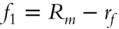 .
.
Table 5.1 Traditional covariance matrix of security returns.


… 


… 


… 
… 


… 
Table 5.2 Factorized covariance matrix of security returns.


… … … … … 


- A “size” portfolio, also known as “small minus big” stock returns, that subtracts large-cap stock returns from small-cap returns, recognizing small-cap ability to outperform large cap:
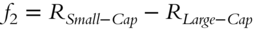 . The “cap” is the capitalization of the company as reflected in its total market valuation (number of stocks issued × price of each stock). Small-cap stocks have historically outperformed large-cap stocks.
 - A “book-to-market” portfolio, also known as “High Minus Low” in reference to the return difference between high book-to-market stocks versus low book-to-market stocks:
 . The book-to-market ratio is calculated as the fraction of accounting value to market value, the latter measured by the stock valuation. Higher book-to-market stocks have been shown to outperform lower book-to-market stocks.
To construct the size and book-to-market portfolios, Fama and French (1992, 1993) sort all the stocks into deciles based on size and book-to-market, respectively. Then, Fama and French create equally weighted size portfolios adding long positions in the smallest by capitalization decile of stocks and shorting the largest decile by capitalization. Similarly, they create the book-to-market portfolios by going long on the highest decile of book-to-market stocks and shorting the lowest decile.
Factorized covariances à la Fan, Fan, and Lv (2008) provide immediate reduction in dimensionality, making the sample covariance matrices suitable for modeling those of the population. Further inversion of factorized, low-dimensional, covariance matrices delivers a sound alternative to the unstable high-dimensional covariance matrices.
Fan, Fan, and Lv's factors are known and may or may not be fully uncorrelated, i.e., orthogonal. In contrast, as shown later in this book, SVD and PCA deliver fully orthogonal factors that arise from the data. These factors, however, may or may not be known to the researchers.
Dimensionality Reduction with Unsupervised Learning
The methodology of Fan, Fan, and Lv (2008) calls on the researchers to determine the factors that are then used to create appropriate portfolios. The resulting factors may not at all represent the optimal factorization. For one, working with large data sets can be very time-consuming. Next, vast computing power may be required to handle the challenge of analyzing all possible factor combinations.
Advances in data processing technology help a bit. For example, researchers may rent powerful servers operated in parallel, hosted in remote locations and accessible online, collectively referred to as being located in a cloud and cloud computing. The servers in a cloud may be organized into interdependent and interoperating groups known as clusters. Each cluster may contain several independent processing nodes (servers, server partitions, or even just processes) capable of handling specific loads. Cluster management systems then may allow the computing load to be dynamically distributed among several nodes, all the while appearing seamless to the end user.
Still, even when equipped with state-of-the-art computing, manually searching for orthogonal factors explaining the data can be a daunting task taking weeks, months, and even years. For example, the best-known factor in Finance, such as Sharpe's (1964) and Lintner's (1965) CAPM, took years to develop and was even awarded a Nobel Memorial Prize in Economics!
UL techniques offer the promise of a fast factor development independent of the researchers. Armed with the latest technology, the factor selection becomes almost instantaneous.
What does UL actually do? By identifying key structural dependencies in the data, unsupervised learning techniques identify latent, unspecified, or previously unknown factors, or combinations of thereof. Furthermore, the factors presented by the UL are orthogonal to each other by construction, freeing the researchers' time from verification of the factors. Further still, the UL factors come ordered from the most globally significant to the least, simplifying the researchers' work even further.
The factors are known as principal components, characteristic values, eigenvalues, or singular values. The corresponding process of distilling the factors is known as principal component analysis (PCA), or singular value decomposition (SVD). Both PCA and SVD work with purely numerical data. Any data containing other-than-numeric values, say, text, have to be converted to the numeric format prior to the analysis.
The key idea behind factorization in either PCA or SVD is to find the dimensions of the data along which the data vary the most and the least. The factors that account for most variation in the data are typically critical to the reconstruction of the entire data set while the factors along which the data vary the least are the ones providing the final touches of detail, and, quite often, noise.

Figure 5.1 Original sample image.
Unsupervised Learning: Intuition via Image Factorization
Many Big Data techniques, such as spectral decomposition, first appeared in the eighteenth century when researchers grappled with solutions to differential equations in the context of wave mechanics and vibration physics. Fourier furthered the field of eigenvalue applications extensively with partial differential equations and other work.
At the heart of many Big Data models is the idea that the properties of every data set can be uniquely summarized by a set of values, called eigenvalues. An eigenvalue is a total amount of variance in the data set explained by the common factor. The bigger the eigenvalue, the higher the proportion of the data set dynamics that eigenvalue captures.
Eigenvalues are obtained via one of the techniques, principal component analysis (PCA) or singular value decomposition (SVD), discussed below. The eigenvalues and related eigenvectors describe and optimize the composition of the data set, perhaps best illustrated with an example of an image.
The intuition on which the technique is based is illustrated with the example from image processing. Consider the black-and-white image shown in Figure 5.1. It is a set of data points, “pixels” in computer lingo, whereby each data point describes the color of that point on a 0–255 scale, where 0 corresponds to pure black, 255 to pure white, and all other shades of gray lie in between. This particular image contains 460 rows and 318 columns.
To perform spectral decomposition on the image, we utilize SVD, a technique originally developed by Beltrami in 1873. For a detailed history of SVD, see Stewart (1993). Principal component analysis (PCA) is a related technique that produces eigenvalues and eigenvectors identical to those produced by SVD, when PCA eigenvalues are normalized. Raw, non-normalized, PCA eigenvalues can be negative as well as positive and do not equal the singular values produced by SVD. For the purposes of the analysis presented here, we assume that all the eigenvalues are normalized and equal to singular values. Later in this chapter, we show why and how PCA and SVD are related and can be converted from one to another.
Singular Value Decomposition
In SVD, a matrix X is decomposed into three matrices: U, S, and V,
where
- X is the original n x m matrix;
- S is an m × m diagonal matrix of singular values or eigenvalues sorted from the highest to the lowest on the diagonal;
- V' is the transpose of the m x m matrix of so-called singular vectors, sorted according to the sorting of S;
- U is an n × n “user” matrix containing characteristics of rows vis-à-vis singular values.
SVD delivers singular values sorted from the largest to the smallest. The plot of the singular values corresponding to the image in Figure 5.1 is shown in Figure 5.2. The plot of singular values is known as a “scree plot” since it resembles a real-life scree, a rocky mountain slope.
A scree plot is a simple line segment plot that shows the fraction of total variance in the data as explained or represented by each singular value (eigenvalue). The singular values are ordered and assigned a number label, by decreasing order of contribution to total variance.
To reduce the dimensionality of a data set, we select k singular values. If we were to use the most significant of the singular values, typically containing macro information common to the data set, we would select the first k values. However, in applications involving idiosyncratic data details, we may be interested in the last k values, for example, when we need to evaluate the noise in the system. A rule of thumb dictates breaking the eigenvalues into sets before the “elbow” and after the elbow sets in the scree plot.
What is the perfect number of singular values to keep in the image of Figure 5.1? An experiment presented in Figures 5.3–5.9 shows the evolution of the data with varying numbers of eigenvalues included. The eigenvalues and the corresponding eigenvectors comprised of linear combinations of the original data create new “dimensions” of data. As Figures 5.3–5.9 show, as few as 10 eigenvalues allow the human eye to identify the content of the image, effectively reducing dimensionality of the image from 318 columns to 10.
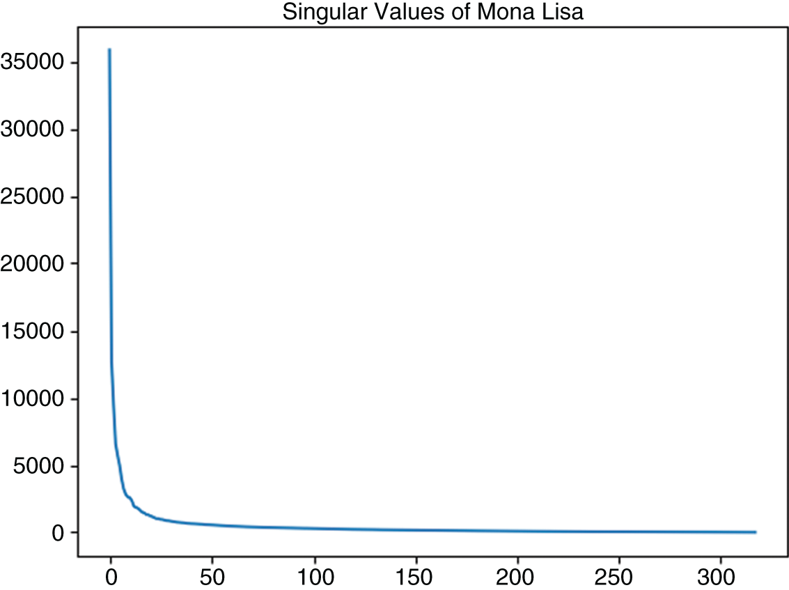
Figure 5.2 Scree plot corresponding to the image in Figure 5.1.
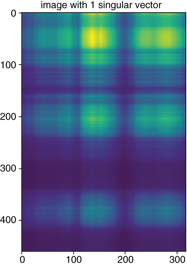
Figure 5.3 Reconstruction of the image of Figure 5.1 with just the first singular value.
However, the guesswork is not at all needed, as numerous methods of selecting the right cut-off value for the eigenvalues have already been researched. Chapter 7 discusses the methodologies for optimal scree plot “elbow” selection using the Marcenko-Pastur theorem.
To create the reduced data set, we restrict the number of columns in the S and V matrices to k by selecting k first elements, determined by the spectral cut-off method. The resulting matrix ![]() has dimensions n rows and k columns, where
has dimensions n rows and k columns, where
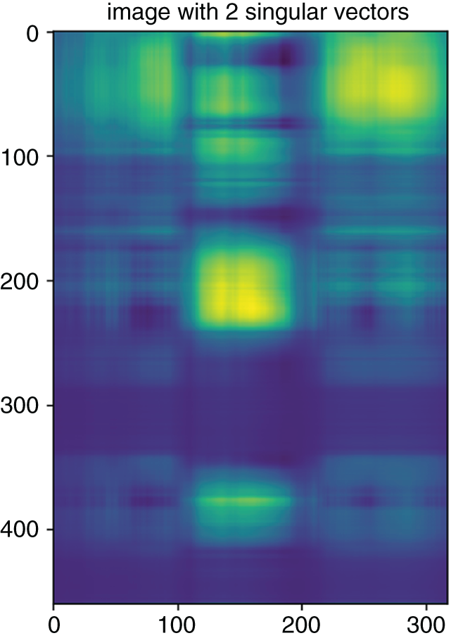
Figure 5.4 Reconstruction of the image in Figure 5.1 with the first 2 singular values.

Figure 5.5 Reconstruction of the image of Figure 5.1 with the first 5 singular values. The outlines of the figure are beginning to appear.
and the unwanted or “cut-off” eigenvalues are replaced by zeros on the diagonal of the![]() matrix.
matrix.
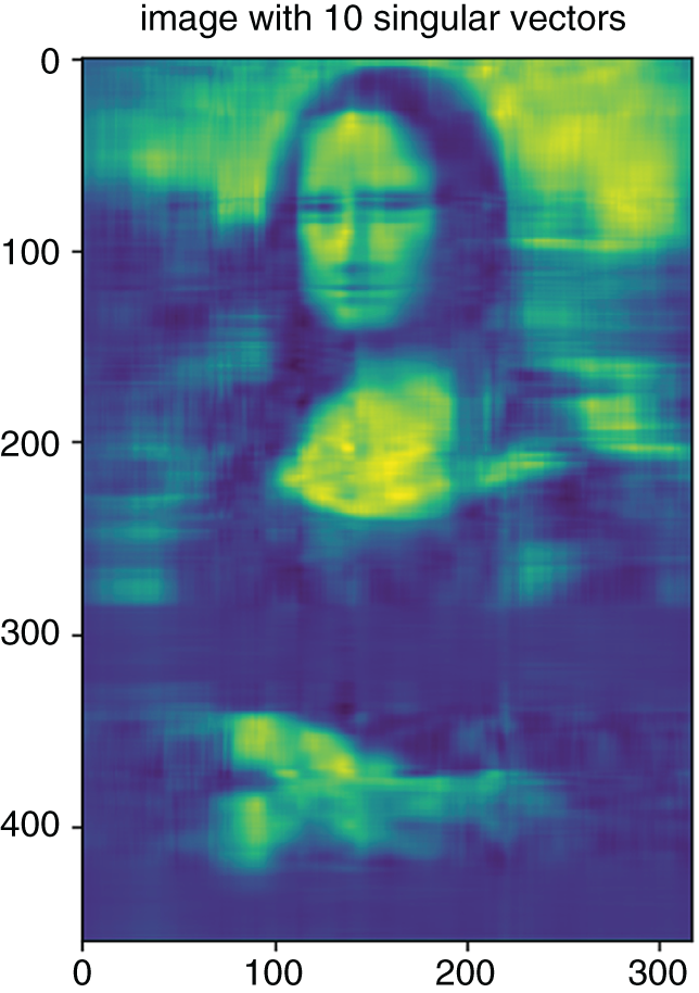
Figure 5.6 Reconstruction of the image in Figure 5.1 with the first 10 singular values.

Figure 5.7 Reconstruction of the image in Figure 5.1 with the first 20 singular values.
The process of reducing the dimensionality of data by essentially wiping out a portion of eigenvalues and the associated eigenvectors is referred to as “whitening.”
As the images above illustrated, Big Data techniques like SVD and PCA masterfully reduce the dimension of the data without sacrificing data quality and the following inferences.
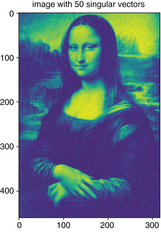
Figure 5.8 Reconstruction of the image in Figure 5.1 with the first 50 singular values.
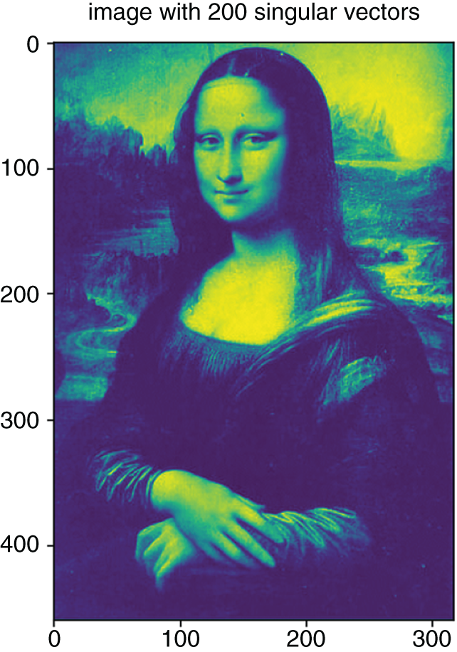
Figure 5.9 Reconstruction of the image in Figure 5.1 with the first 200 singular values.
Why reduce dimensions? Why not use the entire data set available? Many financial applications use daily data. Daily data suffer from relatively small sample size. Take three years of data and you are already counting 750 daily observations, corresponding to 750 rows in a matrix. If you are dealing with, say, 10 or even 50 stocks in portfolio allocation, organized in columns, then traditional covariance-based models will work just fine. However, if your mandate is to optimize a portfolio of the instruments comprising the S&P 500, S&P 1500, Russell 3000, or the entire trading universe, the covariance computation fails. Seminal studies like Johnstone (2001) showed that when the data dimensionality (the number of columns) approaches, not to mention exceeds, the sample size (the number of rows), the sample covariance matrix suffers considerably and is no longer a good estimator for the true population covariance.
Dimensionality reduction, however obvious and easy to grasp an application, is only a small subset of applications of SVD discussed in this book along with applications of PCA and other Big Data tools. Understanding the mechanics of SVD, therefore, is desirable and allows researchers to produce new innovative ideas. SVD, PCA, and several other key tools, like norms, are discussed in detail in the rest of this chapter.
Deconstructing Financial Returns
What do the U, S, and V matrices represent in practice? Consider the case of financial returns.
UL techniques distill the data down to a spectrum of influencing factors. The resulting factors are dependent on the specifics of the problem under consideration. Some of the frequent factors can be movements of the larger markets, others are characteristics of the financial instruments under consideration, and some may even turn out to be returns of other securities.
To determine significant factors driving the data, we rely on a technique known as principal component regression. In a principal component regression, the dependent variable is regressed not on other variables in the data set, but on linear combinations of these variables as determined by top eigenvalues and eigenvectors. Eigenvalues and eigenvectors can be thought of as the core representation of the data, or its most important characteristics. The motivation behind the principal component regression then is to elucidate the dependent variable's characteristics vis-à-vis these powerful singular value-driven factors.
What drives the U.S. equities markets? Here we present a toy example of dimensionality reduction for portfolio allocation and illustrate its performance. To assess, we start with the entire U.S. equities and Electronically Traded Funds (ETFs) universe, which on February 1, 2020, comprised 8,315 names, according to NASDAQ. To ensure a multi-year analysis, we restrict the sample to securities with a three-year or longer history, even though doing so potentially induces a survivorship bias à la Brown, Goetzmann, Ibbotson, and Ross (1992). Removing the names with less than three years of daily data left a sample of 5,983 observations.
Breaking up the sample into 100-stock groups, we perform an in-sample decomposition of returns via SVD on each group over the entire 2018, comprising 251 daily observations. The returns for each security i are computed as simple daily returns, ![]() , where
, where ![]() is a closing price for a stock i on day t. The returns for every 100 stocks are arranged in an n × m matrix with n = 251 days in rows and m = 100 stocks in columns.
is a closing price for a stock i on day t. The returns for every 100 stocks are arranged in an n × m matrix with n = 251 days in rows and m = 100 stocks in columns.
Each 251 × 100 matrix, representing a group of 251 daily returns for 100 stocks, was decomposed using SVD into matrices ![]() ,
, ![]() , and
, and ![]() . The matrix S is diagonal, that is, it is zeros everywhere except on the diagonal. The diagonal of S contains the singular values of the matrix, ordered from the largest to the smallest. The 100 × 1 vectors comprising the
. The matrix S is diagonal, that is, it is zeros everywhere except on the diagonal. The diagonal of S contains the singular values of the matrix, ordered from the largest to the smallest. The 100 × 1 vectors comprising the ![]() matrix are known as the singular vectors and are the factors driving each given set of returns. All the columns of
matrix are known as the singular vectors and are the factors driving each given set of returns. All the columns of ![]() , the singular vectors, are completely uncorrelated with each other, or orthogonal to each other, by construction, as discussed later in this chapter. The singular vectors, like their corresponding singular values, are ordered from the most impactful on the global return scale to the least impactful. The least important singular vectors are often considered to represent the qualities pertaining to the individual stocks, known as idiosyncratic properties.
, the singular vectors, are completely uncorrelated with each other, or orthogonal to each other, by construction, as discussed later in this chapter. The singular vectors, like their corresponding singular values, are ordered from the most impactful on the global return scale to the least impactful. The least important singular vectors are often considered to represent the qualities pertaining to the individual stocks, known as idiosyncratic properties.
The first singular vector is the most impactful across all the securities in the group. It is a linear combination of the returns series in the original returns matrix. Each value of the 100 within the first singular vector corresponds to the coefficient with which the given stock's returns vector is included in the singular vector. To illustrate the output of SVD, Table 5.3 shows the most positive and the most negative return contributions, as determined by SVD, in a portfolio composed from the first 100 stocks.
It is interesting to note that ETFs and pharmaceutical companies dominate the positive and the negative ends of the first singular vector. Similar results can be observed in the other 100-share groups. For example, Table 5.3 shows the most common securities that appeared as the top influencers in the singular value decomposition when all the traded securities were randomly drawn into groups of 200 with replacement. Here, the process of random 200-stock portfolio construction was repeated 1,000 times.
What are the top drivers of the random portfolios? Table 5.4 shows the names of securities that appeared at least twice as the highest coefficient in the first singular vector in 1,000 randomly picked portfolios. The portfolios were chosen randomly with replacement from the universe of all the securities traded in the United States over the 2018–2019 period.
As Table 5.4 shows, 12 out of 31 security names that appear at least in two portfolios as the top influencer in the top singular vector are ETFs or ETNs. In other words, even in a perfectly random portfolio, we have a decent chance of finding an ETF that well represents the underlying returns.
Why is this significant? As shown in Avellaneda and Lee (2010), in times of downward volatility, many investors would like to sell their portfolio holdings at the same time. In many cases, this results in severe liquidity shortages. To overcome the issue, investors sell the most liquid security available, such as NYSE:SPY. Next, the investors gradually rebalance their portfolios to buy back the liquid security and sell their actual portfolio holdings. The resulting approach allows investors to lock in the effects of the downward volatility and mitigate their losses. As Aldridge (2016) shows, the approach has been growing in popularity, as demonstrated by the ever increasing correlations between downward volatility and traded volume of NYSE:SPY (Figure 5.10). Identifying the exact ETF driving the portfolio may deliver more precise outcomes in times of downward volatility than a blanket sell-off of NYSE:SPY.
Table 5.3 Proportions of individual stock returns in the A-AEF Group (100 stocks) included in the first singular vector, as determined by SVD.
| Stock symbol | Description | Proportion in the first singular vector |
|---|---|---|
| Most positive | ||
| ACWI | The iShares MSCI ACWI ETF seeks to track the investment results of an index composed of large and mid-capitalization developed and emerging market equities | 0.3718 |
| ACRX | AcelRx Pharmaceuticals, Inc., a specialty manufacturer of treatments for acute pain | 0.3367 |
| ADME | Aptus Drawdown Managed Equity ETF, that seeks out US stocks exhibiting strong yield plus growth characteristics, and includes market hedges | 0.2706 |
| ADMP | Adamis Pharmaceuticals Corporation, a specialty manufacturer of treatments for respiratory disease and allergies | 0.2076 |
| ACNB | ACNB Corporation, a parent holding company for Russell Insurance Group, Inc., ACNB Bank, Bankersre Insurance Group, Spc | 0.2034 |
| ACRS | Aclaris Therapeutics, Inc., manufacturer of specialty treatments in dermatology, both medical and aesthetic, and immunology | 0.1116 |
| ADSK | Autodesk, Inc., a maker of software for the architecture, engineering, construction, manufacturing, media, education, and entertainment industries | 0.1107 |
| ACN | Accenture plc, a Fortune 500 professional services company that provides services in strategy, consulting, digital, technology, and operations. | 0.1013 |
| ACSI | American Customer Satisfaction ETF, that seeks to track the performance, before fees and expenses, of the American Customer Satisfaction Investable Index | 0.0987 |
| ACU | Acme United Corporation, a supplier of cutting, measuring, and safety products for the school, home, office, hardware, and industrial markets | 0.0972 |
| Most negative | ||
| ACST | Acasti Pharma, a specialty manufacturer of cardiovascular treatments | -0.3473 |
| ACT | AdvisorShares Vice ETF, tracking select alcohol and tobacco companies | -0.2409 |
| ADMS | Adamas Pharmaceuticals, a specialty manufacturer of treatment for chronic neurological diseases | -0.2226 |
| ACOR | Acorda Therapeutics, Inc., a specialty manufacturer of neurology therapies for Parkinson's disease, migraine, and multiple sclerosis | -0.2057 |
| ACWX | iShares MSCI ACWI ex U.S. ETF, tracking large and mid-cap equities outside of the U.S. | -0.1903 |
| ADES | Advanced Emissions Solutions, Inc., a holding company for a family of companies that provide emissions solutions to customers in the coal-fired power generation, industrial boiler, and cement industries | -0.1485 |
| ADNT | Adient PLC, a manufacturer of automotive seating for customers worldwide | -0.1368 |
| ACH | Aluminum Corporation of China Limited, the world's second-largest alumina producer and third-largest primary aluminum producer at the time this book was written | -0.1331 |
| ACP | Aberdeen Income Credit Strategies Fund, a non-diversified, closed-end management investment company | -0.1265 |
| ADRE | Invesco BLDRS Emerging Markets 50 ADR Index Fund | -0.1054 |

Figure 5.10 Rolling 250-day correlations between intraday downward volatility and volume of NYSE:SPY. Based on Aldridge (2016).
For instance, in the initial days of the COVID-19 crisis emergence in the United States, investment professionals struggled to unload investments quickly in a rapidly declining market. The example below illustrates a practical way to hedge the sell-off by selecting and selling the most appropriate ETF, and then gradually rebalancing the portfolio to their desired composition.
Table 5.4 The most common top positive factors in the first singular value out of 10,000 portfolios of 200 stocks each selected randomly with replacement from the entire universe of securities traded in the U.S. for the 2018 calendar year.
| Symbol | Name | Sector |
|---|---|---|
| ICOL | iShares MSCI Colombia ETF (ICOL) | ETF |
| CHD | Church & Dwight Co., Inc. (CHD) | Consumer Defensive, Household & Personal Products |
| DJP | iPath Bloomberg Commodity Index Total Return (SM) ETN (DJP) | ETN |
| AGEN | Agenus, Inc. (AGEN) | Healthcare, Biotechnology |
| EDU | New Oriental Education & Technology Group, Inc. (EDU) | Consumer Defensive, Education & Training Services |
| VER | VEREIT, Inc. (VER) | Real Estate, REIT—Diversified |
| ECH | iShares MSCI Chile Capped ETF (ECH) | ETF |
| KEP | Korea Electric Power Corporation (KEP) | Utilities, Utilities—Regulated Electric |
| NEOS | Neos Therapeutics, Inc. (NEOS) | Healthcare, Drug Manufacturers—Specialty & Generic |
| XWEB | SPDR S&P Internet ETF (XWEB) | ETF |
| EEMV | iShares Edge MSCI Min Vol Emerging Markets ETF (EEMV) | ETF |
| PSMB | Invesco Balanced Multi-Asset Allocation ETF (PSMB) | ETF |
| TDW | Tidewater, Inc. (TDW) | Energy, Oil & Gas Equipment & Services |
| OII | iPath Series B S&P GSCI Crude Oil Total Return Index ETN (OIL) | ETN |
| DLX | Deluxe Corporation (DLX) | Communication Services, Advertising Agencies |
| ADRO | Aduro BioTech, Inc. (ADRO) | Healthcare, Biotechnology |
| PNI | PIMCO New York Municipal Income Fund II (PNI) | ETF |
| MPB | Mid Penn Bancorp, Inc. (MPB) | Financial Services, Banks—Regional |
| NAT | Nordic American Tankers Limited (NAT) | Industrials, Marine Shipping |
| FLTR | VanEck Vectors Investment Grade Floating Rate ETF (FLTR) | ETF |
| BKI | Black Knight, Inc. (BKI) | Technology, Software—Infrastructure |
| NMRK | Newmark Group, Inc. (NMRK) | Real Estate, Real Estate Services |
| VRTV | Veritiv Corporation (VRTV) | Industrials, Business Equipment & Supplies |
| JAN | JanOne, Inc. (JAN) | Industrials, Waste Management |
| IAT | iShares U.S. Regional Banks ETF (IAT) | ETF |
| DCP | DCP Midstream, LP (DCP) | Energy, Oil & Gas Midstream |
| DEUR | Citigroup ETNs linked to the VelocityShares Daily 4X Long USD vs. EUR Index (DEUR) | ETN |
| ZEUS | Olympic Steel, Inc. (ZEUS) | Basic Materials, Steel |
| BOXL | Boxlight Corporation (BOXL) | Technology, Communication Equipment |
| REDU | RISE Education Cayman Ltd (REDU) | Consumer Defensive, Education & Training Services |
| RVRS | Reverse Cap Weighted U.S. Large Cap ETF (RVRS) | ETF |
Table 5.5 Correlation of the top-ten eigenvectors of the Russell 3000 stocks with ETFs (highest and lowest ETF correlation shown) and Fama-French factors in 2018 (Fama and French 1992, 1993).
| # Eigenvector | Maximum Correlation ETF (%) | Minimum Correlation ETF (%) | Correlation with Excess Market R (%) | Correlation with SMB (%) | Correlation with HML (%) |
|---|---|---|---|---|---|
| 1 | 18.1, ACH | −19.1, AACG | 6.6 | −2.2 | 2.4 |
| 2 | 44.0, AFB | −25.1, ABEV | 12.8 | 1.2 | −1.5 |
| 3 | 21.0, AGG | −49.4, ADRA | −11.6 | 0.0 | −1.7 |
| 4 | 58.5, AGGE | −47.7, AGT | −2.0 | −3.0 | 2.5 |
| 5 | 24.4, AGZ | −24.0, AZUL | 2.9 | 15.3 | −5.9 |
| 6 | 17.1, BSCM | −20.6, EDEN | 2.3 | 7.9 | 1.3 |
| 7 | 25.6, GDO | −19.7, EZT | 4.9 | 5.0 | 4.2 |
| 8 | 15.6, AB | −18.2, WPP | 1.1 | −1.3 | −1.8 |
| 9 | 22.5, ABEV | −21.2, AACG | 7.8 | −8.3 | −2.8 |
| 10 | 26.8, ACT | −24.5, AAXJ | 4.6 | 2.9 | −2.6 |
Why is selection of the best-fit ETF a problem warranting its own solution? As discussed earlier in this chapter, selling SPY in times of downward volatility has become a go-to strategy for portfolio managers. In times of crises, when most of the investors rush over to short SPY, doing so becomes unreasonably expensive. Separately, the number of ETFs has exploded in recent years. As of January 2020, for example, the Boston Stock Exchange has traded 5,179 stocks and 4,176 non-stock issues, including ETFs, electronically-traded notes (ETNs), and American Depository Receipts (ADRs), the latter being proxies for the foreign-traded shares. With the number of non-corporate securities rapidly approaching and even threatening to exceed the number of publicly traded shares, there may be a reasonably-priced SPY alternative for pretty much most equity portfolios!
As Table 5.5 shows, ETFs dominated Russell 3000 in 2018. Returns on certain ETFs like AGGE, ADRA, and AGT were highly positively and negatively correlated with returns composed of eigenvector allocations based on dimensionality reduction of Russell 3000 returns. The highest positive correlation was due to AGGE (IQ Enhanced Core Bond U.S. ETF that ceased trading on February 4, 2020, according to ET.com), followed by AFB (AllianceBernstein National Municipal Income Fund). AGGE showed 58.5% correlation with the fourth eigenvector-portfolio of Russell 3000 returns in 2018 while AFB registered 44% correlation with the second eigenvector of the Russell 3000 returns. The funds most negatively correlated with the Russell 3000 eigenvectors were ADRA (Invesco BLDRS Asia 50 ADR Index Fund, ceased trading on February 14, 2020) and AGT (iShares MSCI Argentina and Global Exposure ETF). ADRA showed -49.4% correlation with the third eigenvector of Russell 3000, and AGT delivered -47.7% with the fourth eigenvector.
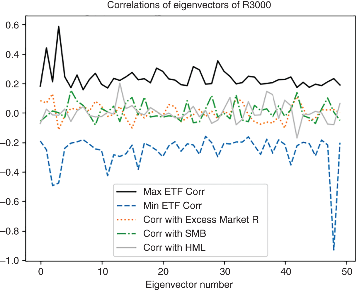
Figure 5.11 2018 returns' eigenvectors' correlation with contemporaneous Fama-French factors and all contemporaneous ETFs.
To benchmark the factor correlations, we compare that with the correlations of the Fama and French factors. According to the Fama and French classic three-factor model (Fama and French 1992, 1993), financial returns can be explained by:
- excess market return (Rm - Rf)
- growth: HML (“High Book-to-Value Minus Low Book-to-Value” portfolio returns)
- size: SML (“Small Minus Large” portfolio returns).
As shown in Table 5.5 and Figure 5.11, the highest Fama-French factor correlations were reached by the excess market return with the second eigenvector portfolio of the Russell 3000 returns (12.8%), SMB with the fifth eigenvector portfolio (15.3%), and HML with the seventh eigenvector portfolio (just 4.2%). Potentially, the dominance of ETFs can explain the increasingly poor performance of the Fama-French factors, documented on the Kenneth French website (https://mba.tuck.dartmouth.edu/pages/faculty/ken.french/data_library.html).
Why did AGGE and ADRA shut down? The coronavirus COVID-19 crisis was sweeping the world in February 2020. AGGE and ADRA perhaps wisely stopped operating to avoid catastrophic losses. However, AFB only lost 22% while the S&P 500 was down 33% of its pre-crisis high. AGT, on the other hand, lost 45% of value in a span of a few days. Also, while the sell-off in SPY and AGT began on February 20, 2020, AFB held strong through March 6. All three securities reached the bottom on March 23, 2020.
Table 5.5 further compares COVID-crisis performance of the top-five ETFs most positively and negatively correlated with the top eigenvectors of the Russell 3000 index. As Table 5.5 shows, the most positively correlated ETFs have largely retained their value through the crisis while the most negatively correlated ETFs lost an extreme proportion of their equity, often way in excess of the -32.10% drop in the S&P 500 over Feb. 20–Mar. 23, 2020. It is likely that the top positively correlated ETFs indeed will capture the core structure of the Russell 3000 and retain a higher proportion of their values in crises.
Table 5.6 Covid crisis performance of the ETFs most correlated with the top-ten eigenvectors of the Russell 3000.
| # Eigenvector | Maximum Correlation ETF | Minimum Correlation ETF |
|---|---|---|
| 1 | ACH Jan. 6–Mar. 26, 2020, -48.05% |
AACG Oct. 2019–Mar. 23, 2020, -60.0% |
| 2 | AFB Mar. 6–Mar. 23, 2020, -23% |
ABEV Jan. 2–Mar. 16, 2020, -55.39% |
| 3 | AGG March 9–18, 2020, -8.6% |
ADRA Stopped trading Feb. 14, 2020 |
| 4 | AGGE Stopped trading Feb. 4, 2020 |
AGT Feb. 20–Mar. 20, 2020, -45.08% |
| 5 | AGZ Feb. 6–Mar. 9, 2020, +4.3% |
AZUL Feb. 5–Mar. 18, 2020, -86.16% |
Interestingly, the top positively correlated issue was an ADR for Aluminum Corporation of China Limited (ACH), which understandably performed poorly due to the economic devastation in China. At the same time, the next top issues were all bond funds: AllianceBernstein National Municipal Income Fund (AFB), iShares Core U.S. Aggregate Bond ETF (AGG), IQ Enhanced Core Bond U.S. ETF (AGGE), and iShares Agency Bond ETF (AGZ).
On the negative correlation side, the top funds covered emerging markets, in a sense, the antithesis of Russell 3000: ATA Creativity Global (AACG), a Chinese education company, Ambev S.A. (ABEV), a Brazilian beverage manufacturer, Invesco BLDRS Asia 50 ADR Index Fund (ADRA), iShares MSCI Argentina and Global Exposure ETF (AGT), and Azul S.A. (AZUL), a Brazilian airline. Figures illustrate the performance of the top issues positively correlated (“good”) and negatively correlated (“bad”) with the top-five eigenvectors of the Russell 3000 returns (Table 5.6) (Figures 5.12 and 5.13).
The application of the principal component regression presented here illustrates an investment strategy that dives into the “surrogate” core structure issues of financial data. Instead of investing in the Russell 3000 itself, we consider the proxies for the drivers of the Russell 3000 returns. Investing in the core drivers delivered relative stability in the COVID-19 crisis. Overall, issues like China Aluminum have delivered growth (until the crash) while the bond funds buoyed the portfolio. Avoiding issues negatively correlated with the top eigenvectors helps to further bullet-proof the portfolio against the crises.
Figures 5.14 and 5.15 further show performance of the “good” and “bad” ETFs selected based on 2018 data through 2019 and the COVID crisis. As Figures 5.14 and 5.15 show, ACH indeed led SPY throughout 2019 and early 2020.
Using Singular Vectors as Portfolio Weights
Since singular vectors represent the core of the data, it is natural to ask whether they can be used in portfolio construction. Can the weights of the individual securities forming the first singular vector or vectors in proxying their respective 100-stock groups be used to form portfolios of stocks that outperform the market? Since these weights represent the dominant drivers of the returns of the 100 stocks, shouldn't the portfolio with these weights outperform the equally weighted portfolio?

Figure 5.12 January–April 2020 Performance of the issues most positively correlated with the top-five eigenvectors of the Russell 3000. Except for Aluminum Corporation of China Limited (ACH), most outperformed the S&P 500 during the COVID crisis.

Figure 5.13 January–April 2020 Performance of the issues most negatively correlated with the top-five eigenvectors of the Russell 3000. All underperformed the S&P 500 during the COVID crisis.
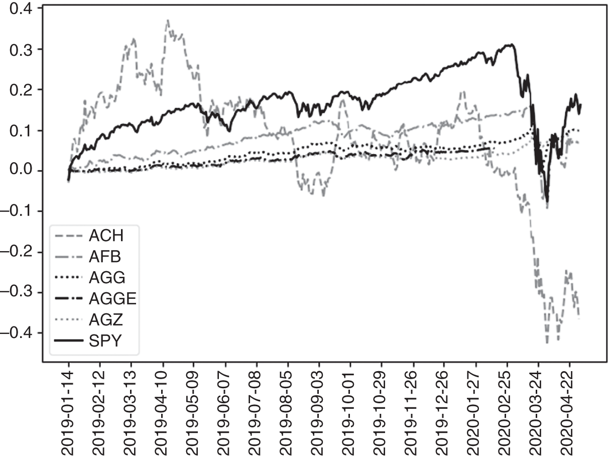
Figure 5.14 January 2019-April 2020 Performance of the issues most positively correlated with the top five eigenvectors of the Russell 3000.

Figure 5.15 January 2019-April 2020 Performance of the issues most negatively correlated with the top five eigenvectors of the Russell 3000.
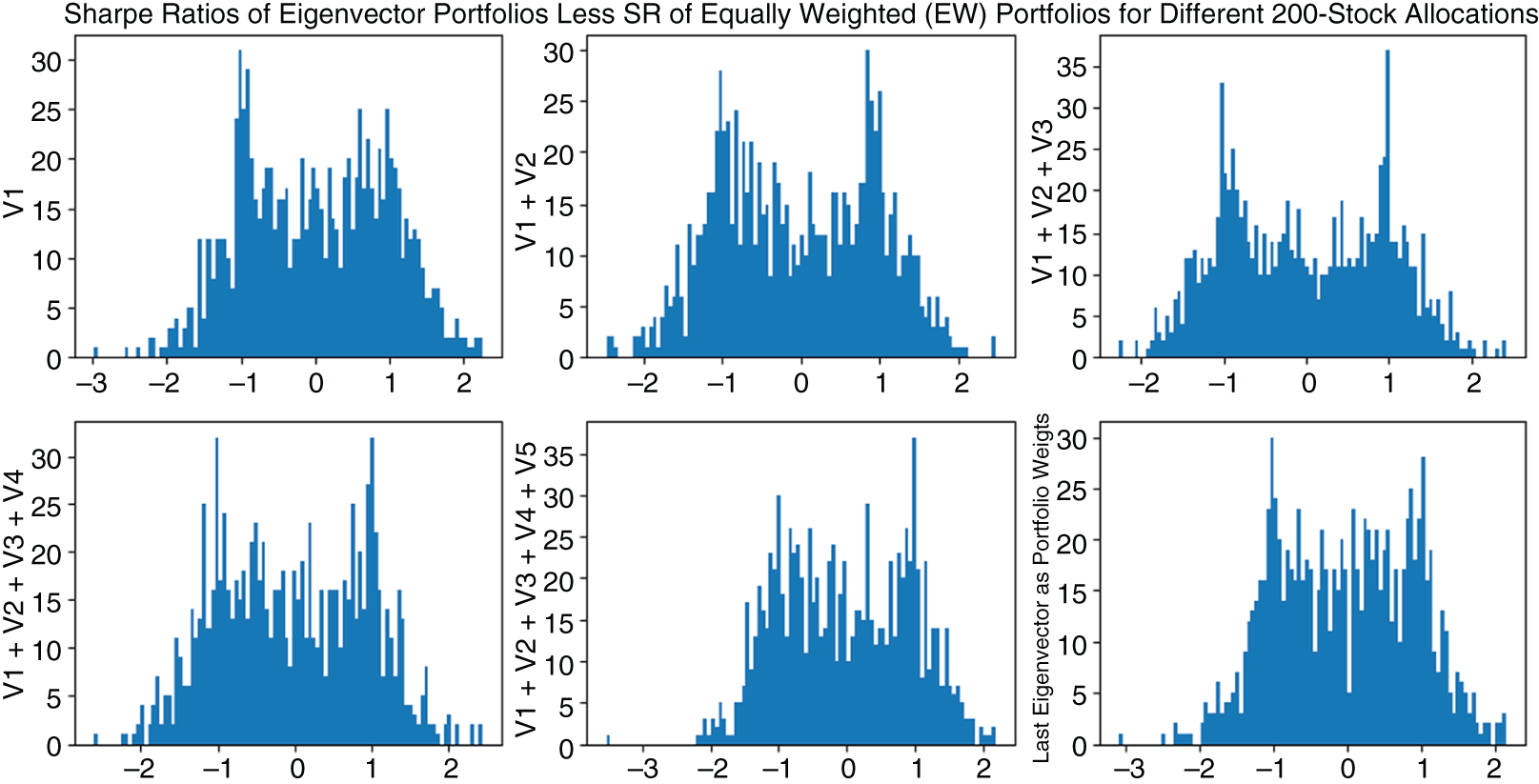
Figure 5.16 Distribution of Excess Sharpe ratios (SR of Portfolio less SR of the Equally Weighted Portfolio) of 1,000 random portfolios allocated according to the coefficients of their returns' first 5 singular vectors and the very last singular vector. All the portfolio Sharpe ratios are adjusted by their Equally Weighted Sharpe ratio.
As Figure 5.16 shows, the portfolios based on top singular vectors of their returns have a bimodal distribution and do not necessarily outperform equally weighted allocation on the respective securities. Specifically, portfolios in Figures 5.10–5.13 were constructed by drawing 200 random names from the entire universe of securities traded in the United States. The instruments that were not traded for the entire 2018–2019 span were next removed from the portfolios. For each of the resulting portfolios, the singular vectors were calculated over the 2018 returns. The performance shown was determined in-sample over the 2018 data, with the weights of the top-5 singular vectors as well as the very last singular vector serving as the weights of the portfolios under consideration.
As Figures 5.17 and 5.18 show, positive and negative singular vectors deliver portfolios that are positively and negatively correlated with the benchmarks, such as the equally weighted portfolio. Long-only portfolios consisting of just positive elements of the first 5 and the very last singular vectors are positively correlated with the equally weighted portfolios made up of the same elements. Short-only portfolios that include just negative elements of the first 5 and the last singular vectors are negatively correlated with the equally weighted portfolios.
Factorized portfolios show that, as the number of singular vectors comprising the portfolios increases, the average returns decrease. At the same time, the return variances decrease as well, resulting in stable, slightly positive Sharpe ratios (Figure 5.19).
Of course, the classic portfolio management theory relates the optimal portfolio construction to the covariance and correlations of returns, not returns themselves. The technique of eigenportfolios, discussed in detail in Chapter 6, applies dimensionality reduction to large correlation matrices. The key idea there is that the correlation data may not be driven by all the correlations in the matrices. Preserving the most important correlations and removing some of the less important correlations allow us to overcome the dimensionality curse as well as produce stable results. As a result of such an application, the computational time required for trading, portfolio management, and risk management applications may be substantially reduced.
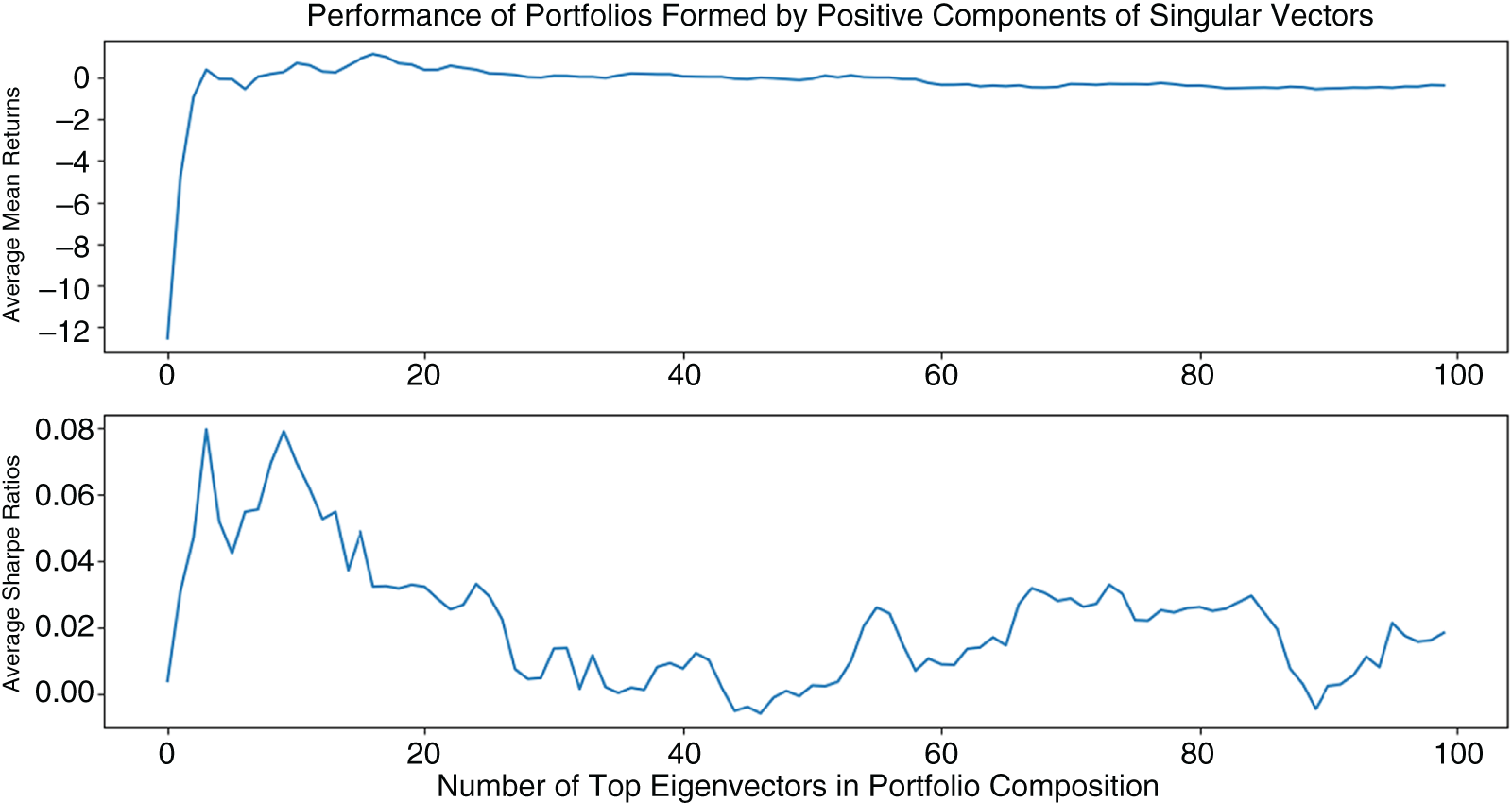
Figure 5.17 Average performance of 1,000 of positive-only components of 1–50 singular vectors. Portfolios consisting of only positive components around 40 singular vectors outperform as measured by mean Sharpe ratios.
Principal Component Regression
Another application of dimensionality reduction is principal component regression, also known as eigenregression. In a principal component regression, the dependent variable is regressed not on other variables in the data set, but on linear combinations of these variables as determined by top eigenvalues and eigenvectors. This approach is particularly useful when the sample is short, relative to its number of features, that is, when the sample has a low rank. Traditional econometric modeling stumbles in this situation, but principal component analysis allows the key relationships in the features (columns of the data) to be condensed into a tightly packed wad of information.
Eigenvalues and eigenvectors can be thought of as the core representation of the data, or its most important characteristics. The motivation behind the principal component regression then is to elucidate the dependent variable's characteristics vis-à-vis these powerful eigenvalue-driven factors.
As an example of an application of the principal component regression, consider financial data analysis that covers the entire healthcare industry (665 stocks), but only over the past quarter (63 trading days). A traditional econometrician would insist that no such analysis can be performed on data with fewer than 665 daily observations. The principal component regression, however, allows us to intelligently compress the number of stocks into its most meaningful portfolios and analyze the latter over a much shorter time interval.
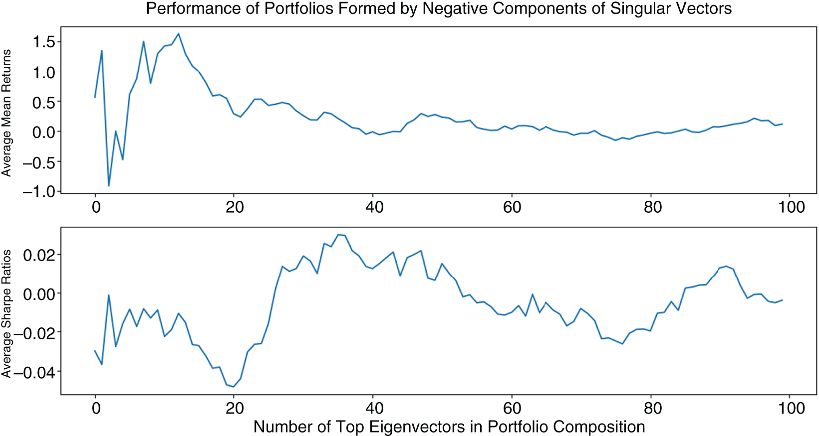
Figure 5.18 Average performance of 1,000 of negative-only components of 1–100 singular vectors. Portfolios consisting of only positive components around 40 singular vectors outperform as measured by mean Sharpe ratios.
Key Big Data Tools: SVD and PCA in Detail
Singular value decomposition (SVD) was briefly introduced in the previous section. Here, we dive in depth into some of the key tools and techniques that will be used throughout much of the book. To showcase the usefulness of the tools, they are presented in the context of a meaningful application: dimensionality reduction.
The power of dimensionality reduction via SVD was graphically illustrated in the previous section. In non-graphical data, dimensionality reduction involves finding a new, smaller set of columns, all of which are some linear combination of the original columns, such that the new column set retains as much data variability and information from the original set as possible. Mathematically, dimensionality reduction is a projection of high-dimensional data onto lower-dimensional data. Given n data points ![]() in
in ![]() , we would like to project the data onto a smaller data set of
, we would like to project the data onto a smaller data set of ![]() dimensions,
dimensions, ![]() . This is very useful when dealing with large unwieldy portfolios like the S&P 500 or Russell 3000. Our objective is to find a d-dimensional projection that preserves as much variance of
. This is very useful when dealing with large unwieldy portfolios like the S&P 500 or Russell 3000. Our objective is to find a d-dimensional projection that preserves as much variance of ![]() as possible.
as possible.
Most PCA- and SVD-based methods operate on the second-moment conditions: they seek to find the orthogonal axes that explain the most data variation.
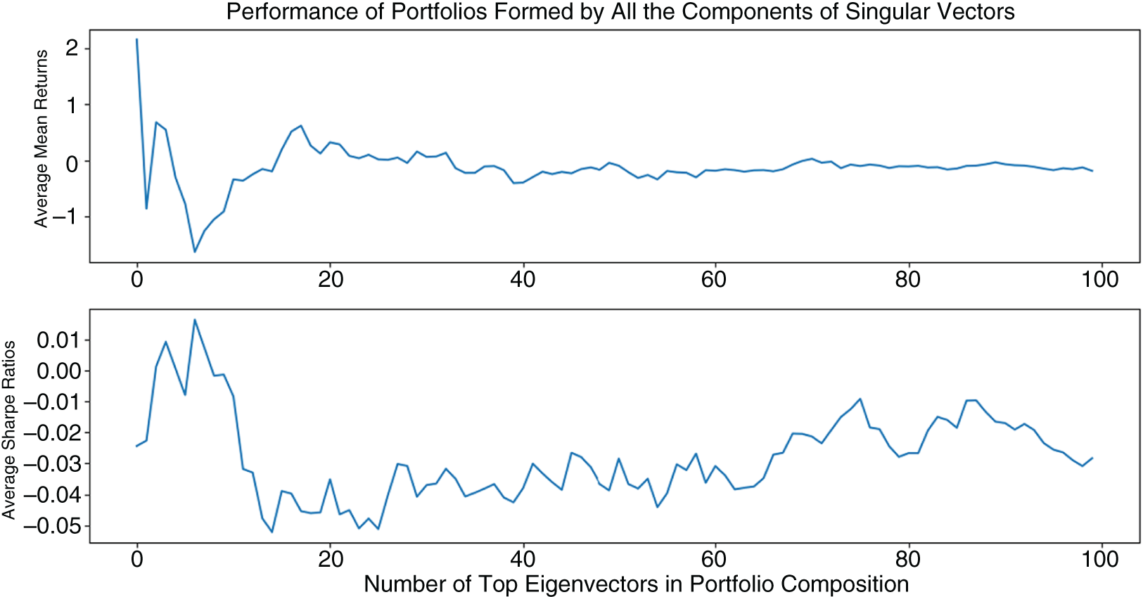
Figure 5.19 Average performance of 1,000 of positive and negative components of 1–100 singular vectors. Portfolios comprising securities weighted by the coefficients of 3 and 4 singular vectors outperform the rest as measured by both the average mean return and the mean Sharpe ratio of the 1,000 random portfolios under consideration. After the fourth singular vector, the portfolio performance drops off sharply in either the mean return, mean Sharpe ratio, or both.
SVD. The SVD of a matrix ![]() is the factorization of
is the factorization of ![]() into three matrices:
into three matrices: ![]() where the columns of
where the columns of ![]() and
and ![]() are orthonormal, and the matrix S is diagonal with positive real entries. The SVD is an important technique for the Big Data Science used extensively throughout this book.
are orthonormal, and the matrix S is diagonal with positive real entries. The SVD is an important technique for the Big Data Science used extensively throughout this book.
The singular value decomposition (SVD) of a matrix ![]() is the factorization of the matrix into the product of three matrices:
is the factorization of the matrix into the product of three matrices:
where all the columns of ![]() and
and ![]() are orthogonal to each other and normalized to be unit vectors, or orthonormal for short, and where the singular value matrix
are orthogonal to each other and normalized to be unit vectors, or orthonormal for short, and where the singular value matrix ![]() is diagonal with real positive values (a diagonal matrix may have non-zero values only on its diagonal, and has zeros everywhere else). The columns of
is diagonal with real positive values (a diagonal matrix may have non-zero values only on its diagonal, and has zeros everywhere else). The columns of ![]() are known as the right singular vectors of
are known as the right singular vectors of ![]() and always form an orthogonal set with no assumptions on
and always form an orthogonal set with no assumptions on ![]() . Similarly, the columns of
. Similarly, the columns of ![]() are known as the left singular vectors of
are known as the left singular vectors of ![]() and also always form an orthogonal set with no assumptions on
and also always form an orthogonal set with no assumptions on ![]() . Due to the orthogonality of
. Due to the orthogonality of ![]() and
and ![]() , whenever the matrix
, whenever the matrix ![]() is square and invertible, the inverse of
is square and invertible, the inverse of ![]() is:
is:
This property becomes very useful in finance applications dealing with matrix inverses, like portfolio management.
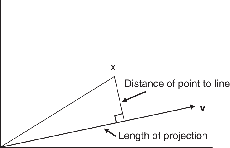
Figure 5.20 An illustration of the relationship between distance of point to line and length of the projection.
In general, however, the matrix ![]() does not need to be square – unlike PCA that requires the input data to be strictly square, SVD happily takes on rectangular matrices. If
does not need to be square – unlike PCA that requires the input data to be strictly square, SVD happily takes on rectangular matrices. If ![]() is
is ![]() , its rows are
, its rows are ![]() points in a
points in a ![]() -dimensional space. SVD then can be thought of as the algorithm finding the best k-dimensional
-dimensional space. SVD then can be thought of as the algorithm finding the best k-dimensional ![]() subspace with respect to the points of
subspace with respect to the points of ![]() . This can be done via best least squares fit by minimizing the sum of the squares of the perpendicular distances of the points to the subspace. An alternative is to find the function to minimize the
. This can be done via best least squares fit by minimizing the sum of the squares of the perpendicular distances of the points to the subspace. An alternative is to find the function to minimize the ![]() axis distance to the subspace of the
axis distance to the subspace of the ![]() .
.
When ![]() , the subspace is a line through the origin. To project the point
, the subspace is a line through the origin. To project the point ![]() onto the line via the best least squares fit, we need to minimize the perpendicular distance of point to line, shown in Figure 5.20. By Pythagoras Theorem,
onto the line via the best least squares fit, we need to minimize the perpendicular distance of point to line, shown in Figure 5.20. By Pythagoras Theorem,
Since ![]() is independent of the line, minimizing (Distance of point to line)2 is equivalent to maximizing the
is independent of the line, minimizing (Distance of point to line)2 is equivalent to maximizing the ![]() .
.
The singular vectors of an ![]() matrix
matrix ![]() are unit vectors
are unit vectors ![]() on the lines through the origin that maximize the lengths of projection for different dimensions. If
on the lines through the origin that maximize the lengths of projection for different dimensions. If ![]() is the ith row of
is the ith row of ![]() ,
, ![]() , then the length of the projection of
, then the length of the projection of ![]() on
on ![]() is
is ![]() . The sum of the lengths squared of all projections is then
. The sum of the lengths squared of all projections is then ![]() . The best fit line maximizes
. The best fit line maximizes ![]() . The Greedy SVD algorithm then works as follows.
. The Greedy SVD algorithm then works as follows.
The first singular vector, ![]() , of
, of ![]() is the best fit line through the origin for the n points in the d-dimensional space that are rows of
is the best fit line through the origin for the n points in the d-dimensional space that are rows of ![]() :
:
The value of ![]() is known as the first singular value of
is known as the first singular value of ![]() ;
; ![]() is the sum of the squares of the projections to the line determined by
is the sum of the squares of the projections to the line determined by ![]() .
.
The second singular vector, ![]() , is defined by the best fit line perpendicular to the first singular vector,
, is defined by the best fit line perpendicular to the first singular vector, ![]() :
:
and the value ![]() is known as the second singular value of
is known as the second singular value of ![]() .
.
The third singular vector, ![]() , is defined by the best fit line perpendicular to the first two singular vectors,
, is defined by the best fit line perpendicular to the first two singular vectors, ![]() and
and ![]() :
:
And the value ![]() is known as the third singular value of
is known as the third singular value of ![]() .
.
The process is repeated until the rth singular vector, ![]() , is found. It can be shown that the number of orthogonal singular vectors of the matrix
, is found. It can be shown that the number of orthogonal singular vectors of the matrix ![]() equals the rank of
equals the rank of ![]() ,
, ![]() .
.
Next, we can define the left singular vectors as ![]() , also orthogonal to each other for
, also orthogonal to each other for ![]() , and formalize the SVD as
, and formalize the SVD as ![]() . From now on, we'll refer to
. From now on, we'll refer to ![]() as right-singular vector.
as right-singular vector.
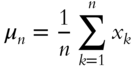
PCA. SVD is a close cousin of PCA. PCA was introduced well over 100 years ago by Pearson (1901). Given the data set ![]() with the sample mean,
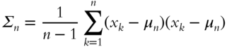
with the sample mean, ![]() , and sample covariance,
, and sample covariance, ![]() shown in Eqs. (5.4) and (5.5), respectively:
shown in Eqs. (5.4) and (5.5), respectively:
Even though the data set ![]() may only be a subset of some larger data distribution, if
may only be a subset of some larger data distribution, if ![]() are sampled independently from that larger distribution, it can be shown that
are sampled independently from that larger distribution, it can be shown that ![]() and
and ![]() are unbiased estimators of the mean and covariance of the larger distribution.
are unbiased estimators of the mean and covariance of the larger distribution.
Formally, PCA's objective is to find the d-dimensional orthonormal basis ![]() , such that the projection of
, such that the projection of ![]() on
on ![]() has the most variance. This is equivalent to seeking the most variance for
has the most variance. This is equivalent to seeking the most variance for ![]() . Hence, our PCA optimization problem becomes:
. Hence, our PCA optimization problem becomes:
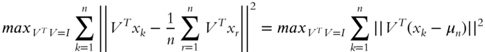
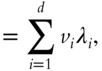
where ![]() are the leading eigenvalues of the sample covariance of
are the leading eigenvalues of the sample covariance of ![]() ,
, ![]() , and
, and ![]() are the associated eigenvectors.
are the associated eigenvectors.
PCA vs. SVD. PCA requires finding the eigenvalues of the covariance of data, ![]() . To do PCA, therefore, one first needs to construct the covariance matrix
. To do PCA, therefore, one first needs to construct the covariance matrix ![]() , which takes 풪
, which takes 풪![]() computational time, and then find the eigenvalues of the covariance matrix in 풪
computational time, and then find the eigenvalues of the covariance matrix in 풪![]() time. The resulting computational complexity of the process is 풪
time. The resulting computational complexity of the process is 풪![]() (see, e.g., Horn and Johnson (1985) and Golub (1996)).
(see, e.g., Horn and Johnson (1985) and Golub (1996)).
SVD, on the other hand, seeks eigenvalues of demeaned data, instead of the covariance matrix. That is, SVD decomposes ![]() into the Unitary vectors
into the Unitary vectors ![]() , a diagonal matrix of singular values S, and singular vectors V, which are identical to the eigenvectors generated by PCA:
, a diagonal matrix of singular values S, and singular vectors V, which are identical to the eigenvectors generated by PCA:
To convert from SVD to PCA is as easy as to observe that, by Eqs. (5.5) and (5.9), the covariance matrix of X is

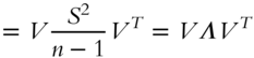
where ![]() are the eigenvalues computed by PCA.
are the eigenvalues computed by PCA.
From Eq (5.10), eigenvalues computed by PCA are ![]() .
.
While we obtain the same result with PCA and SVD, the computational load of SVD, ![]() , is a lot lighter than PCA. An added advantage of SVD vs. PCA is the unitary matrix U, which describes how each row relates to each eigenvector – an added informational dimension.
, is a lot lighter than PCA. An added advantage of SVD vs. PCA is the unitary matrix U, which describes how each row relates to each eigenvector – an added informational dimension.
In addition to being comparatively computationally complex, PCA may cause a loss of precision as well as the outright inability to compute the result. Classic examples like the Läuchli matrix (Läuchli 1967) showcases where PCA fails to converge altogether while SVD delivers solid computation.
Norms. Two important matrix norms, the Frobenius norm, ![]() , and the 2-norm,
, and the 2-norm, ![]() , are also often used throughout this book. The 2-norm,
, are also often used throughout this book. The 2-norm, ![]() , is formally defined as
, is formally defined as
and is thus equal to the largest eigenvalue of ![]() .
.
It can also be shown that the sum of squares of the singular values equals the Frobenius norm squared,
Computing PCA and SVD
Techniques like PCA and SVD are central to data science and help speed up processes and quickly infer meaning by retrieving the structure of the data. Even though PCA and SVD are critical to data scientists today, they originated in the twentieth century. Today, researchers are looking for ways to improve on the traditional PCA and SVD: (i) to speed up the computation further; (ii) to take advantage of the developments in other fields, like Random Matrix Theory, that did not exist when PCA and SVD were created; and (iii) to make PCA and SVD work even more efficiently with today's computational technology that has drastically improved since PCA and SVD first came to light.
Most off-the-shelf programming packages offered built-in PCA and SVD functionality at the time this book was written. However, in many cases, off-the-shelf PCA and SVD calculations take up a significant portion of the programming resources. In some programs, while still drastically outperforming traditional non–Big Data methods, PCA and SVD create bottlenecks, accounting for a disproportionately large calculation time compared to the rest of the data logic.
The computational efficiency of PCA and SVD can be measured by the speed of processing an arbitrarily large data set. After all, isn't this what Big Data is all about? However, in the current advanced, but still growing, power of computing technology, extremely large data sets may still be hard to process. Instead, researchers deploy stochastic techniques to randomly sample the data. These online methods grab a random slice of data, thereby creating a smaller data set that is still representative of the original big data set. Next, PCA or SVD is applied to the smaller data sample, and the sampling process is repeated until a certain stopping condition is met and the results are aggregated. In this approach, the algorithm may process the entire data set or only a portion thereof.
Another metric of the algorithm efficiency is the iteration complexity. Iteration complexity measures the number of loops taken by the algorithm; the fewer the loops, the more efficient the computation. Breaking up the sample and iterating over each piece generates a large number of loops, something that takes up potentially large computational time.
The computational time required to produce SVD estimates depends on the algorithm. The most popular algorithms for SVD over the years have been the power algorithm (Hotelling 1933) and the Lanczos algorithm (Lanczos 1958).
Over the years, researchers have strived to improve the efficiency of PCA and SVD calculations. As a result, several powerful “Golden standard” algorithms emerged and are presented in this section that may or may not be part of the off-the-shelf solutions and may warrant in-house implementation. These algorithms include the power algorithm and its extensions, including a range of Lanczos algorithms, various stochastic approaches, and Fast SVD, discussed in this chapter.
The Power Algorithm for SVD and PCA Estimation. The power algorithm is simple, yet robust and has been extended in many forms over the years and is the basis for many SVD and PCA algorithms. The name “power” refers to the process of self-multiplying matrices, or raising them to a power, in order to determine the singular values and vectors. Here, we first consider a sketch of the case of the power method applied to a square symmetric matrix, and then generalize the result to any ![]() matrix.
matrix.
When matrix ![]() is square symmetric, under certain assumptions, it can be represented as it has the same right and left singular vectors
is square symmetric, under certain assumptions, it can be represented as it has the same right and left singular vectors ![]() :
:

Next,
Since the inner product ![]() whenever
whenever ![]() by orthogonality (the outer product
by orthogonality (the outer product ![]() is not 0),
is not 0),
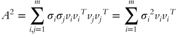
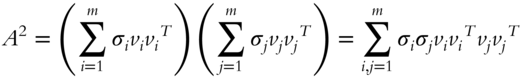
In general, if we raised ![]() to the power
to the power ![]() ,
,

With ![]() ,
,
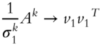
Since ![]() is unknown at this point, we cannot compute
is unknown at this point, we cannot compute ![]() directly. However, dividing
directly. However, dividing ![]() by its Frobenius norm
by its Frobenius norm ![]() results in matrix
results in matrix ![]() converging to the rank 1 matrix
converging to the rank 1 matrix ![]() . From the latter, we can compute
. From the latter, we can compute ![]() .
.
In general, the assumption of a square and symmetric matrix ![]() having the same left and right eigenvectors is too strong. However, we can always find
having the same left and right eigenvectors is too strong. However, we can always find ![]() that satisfies our original assumptions. If
that satisfies our original assumptions. If ![]() can be decomposed, say, via SVD, into
can be decomposed, say, via SVD, into ![]() , then the spectral decomposition of
, then the spectral decomposition of ![]() is:
is:
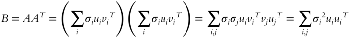
since ![]() for all
for all ![]() due to orthogonality. Furthermore, powering up
due to orthogonality. Furthermore, powering up ![]() produces
produces
![]() if
if ![]()
As ![]() increases, for
increases, for ![]() and
and ![]() ,
, ![]() , and so
, and so
Thus, the power method involves powering up the data in order to determine the associated eigenvalues. The convergence of the power method can be shown to be achieved quickly if there is a significant gap ![]() between the first and the second eigenvalues. Known as the eigen-gap,
between the first and the second eigenvalues. Known as the eigen-gap, ![]() is a common determinant of the speed of SVD and PCA algorithms as it determines the speed with which eigenvalues can be separated from each other. The higher the gap, the easier it is to separate the eigenvalues and reach decomposition.
is a common determinant of the speed of SVD and PCA algorithms as it determines the speed with which eigenvalues can be separated from each other. The higher the gap, the easier it is to separate the eigenvalues and reach decomposition.
Computing ![]() costs
costs ![]() matrix multiplications, or
matrix multiplications, or ![]() , if matrices are multiplied by
, if matrices are multiplied by ![]() once per iteration. To reduce the complexity, successively squaring
once per iteration. To reduce the complexity, successively squaring ![]() lowers the complexity to
lowers the complexity to ![]() . Computing
. Computing ![]() , where
, where ![]() is a randomly chosen unit vector, lowers the complexity further to
is a randomly chosen unit vector, lowers the complexity further to ![]() iterations and can operate in a stochastic sample-driven fashion. The Lanczos method, due to Lanczos (1958), optimizes the power method in the direction of the extreme highest and lowest eigenvalues and typically takes
iterations and can operate in a stochastic sample-driven fashion. The Lanczos method, due to Lanczos (1958), optimizes the power method in the direction of the extreme highest and lowest eigenvalues and typically takes ![]() iterations. Due to its directionality, the Lanczos method needs to work with a full sample, i.e., it cannot work in the online environment.
iterations. Due to its directionality, the Lanczos method needs to work with a full sample, i.e., it cannot work in the online environment.
Optimization of the performance of PCA and SVD calculations was an active area of research at the time this book was written. The algorithm by Liberty, Woolfe, Martinsson, Rokhlin, and Tygert (2007), dubbed Fast SVD, uses Fast Fourier Transform to speed up the computation. Musco and Musco (2015) use bootstrapping via the block Krylov method to derive convergence independent of the eigen-gap ![]() . Bhojanapalli, Jain, and Sanghavi (2015) use alternating minimization to achieve a low-complexity performance in sub-sampling of the matrix. Shamir (2016) proposes a stochastic variance-reduction PCA. Xu, He, De Sa, Mitliagkas, and Ré (2018) propose an extension of the power method, power iteration with momentum, that works online and achieves Lanczos performance of
. Bhojanapalli, Jain, and Sanghavi (2015) use alternating minimization to achieve a low-complexity performance in sub-sampling of the matrix. Shamir (2016) proposes a stochastic variance-reduction PCA. Xu, He, De Sa, Mitliagkas, and Ré (2018) propose an extension of the power method, power iteration with momentum, that works online and achieves Lanczos performance of ![]() iterations.
iterations.
Fast SVD
Fast SVD due to Liberty, Woolfe, Martinsson, Rokhlin, and Tygert (2007), discussed in this section, is one of the recent improvements of the technique. Liberty et al. apply the randomization and Fast Fourier Transform (FFT) to traditional SVD to dramatically increase its computational speed. Due to the application of FFT to randomization, their algorithm also has a finite probability of failure; however, Liberty et al. estimate that this probability is on the order of ![]() .
.
To create the fast version of SVD, Liberty et al. first create interpolative decompositions (IDs), described in this section, and then convert IDs into SVD. An ID is an approximate decomposition of any matrix ![]() of rank
of rank ![]() into a product of two matrices:
into a product of two matrices:
- a subset of matrix
 ,
,  , and
, and - matrix
 , such that, by Lemma (1) in Liberty et al. (2007):
- Some set of the columns of
 makes up an identity matrix
  .
. - The absolute values of all entries of
 are less than or equal to 1
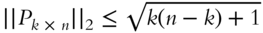
- The least, same as the
 th greatest singular value of
  is at least 1
 - When
 or
or  ,
, 
- When
 or
or  ,
,  , where
  is the
  st greatest singular value of
  .
.
- Some set of the columns of
The approximation ![]() is then numerically stable and is referred to as the interpolative decomposition (ID) of
is then numerically stable and is referred to as the interpolative decomposition (ID) of ![]() .
.
At the core of Liberty et al.'s research is a speedy randomized Discrete Fourier Transform. The transform is a uniform random sampler ![]() of a Discrete Fourier Transform
of a Discrete Fourier Transform ![]() of diagonal matrices
of diagonal matrices ![]() to use in the fast computation of the IDs, following Ailon and Chazelle (2006):
to use in the fast computation of the IDs, following Ailon and Chazelle (2006):
 is a diagonal
  matrix with complex independent and identically distributed random-variable entries
  , distributed uniformly on the unit circle.
 is the
  Discrete Fourier Transform with
 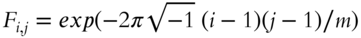 .
. is a real
  matrix, an operator that uniformly randomly selects rows from the product of
  and
and  . As such, all of the entries of
  are 0 except for one 1 in the diagonal in each of the randomly selected columns
  , with
  uniformly drawn with replacement from
  .
.
The resulting speedy randomized Discrete Fourier Transform is an operator
with the cost of applying ![]() to any arbitrary vector via Sorrensen and Burrus (1993) being
to any arbitrary vector via Sorrensen and Burrus (1993) being
Armed with the speedy randomized Discrete Fourier Transform, Liberty et al. (2007) describe two algorithms for Interpolative Decomposition (ID), followed by an algorithm of converting ID into SVD.
Conclusion
PCA and SVD are powerful techniques that allow researchers to distill the structure of the data, identifying key drivers. The drivers let the data speak for themselves, without requiring the researchers to provide traditional hypotheses. The techniques are potentially game-changers in modern finance.
These Big Data methods allow us to process large data sets quickly, without adding computing power, saving corporations millions of dollars by timely short-term identification of impending risk events. The Big Data Science hypothesis-less paradigm further allows more reliable and efficient conclusions to be drawn by removing researchers' subjectivity in posing the research question.
Appendix 5.A PCA and SVD in Python
Both PCA and SVD are easy to program in Python.
To obtain the first five principal components of a dataset X, all one needs to write is the following code:
from sklearn.decomposition import PCApca = PCA(n_components=5)PCs = pca.fit_transform(X)
Of course, PCA is based on analyzing variance of the data, so it helps when all the columns of the data are standardized to approximate the N(0,1) distribution. Luckily for us, the standardization of data is also taken care of in Python and is done with the following code:
from sklearn.preprocessing import StandardScalerX = StandardScaler().fit_transform(X)
Such pre-processing of data is now a standard feature in many applications and produces better predictions than relying on raw data as inputs.
PCA's cousin, SVD, is equally easy to build in Python. The matrices U, S, and V of SVD decomposition of matrix X can be obtained with the following two lines of code:
from scipy import linalgU, s, Vh = linalg.svd(X)
The simplicity and elegance of the Python code make the analysis fast, simple, and even very enjoyable!
For specific code examples, please visit https://www.BigDataFinanceBook.com, and register with password SVD (case-sensitive).
References
- Ailon, N. and Chazelle, B. (2006). Approximate nearest neighbors and the fast Johnson-Lindenstrauss transform. In: Proceedings of the Thirty-Eighth Annual ACM Symposium on the Theory of Computing, 557–563. New York: ACM Press.
- Aldridge, I. (2016). ETFs, high-frequency trading, and flash crashes. The Journal of Portfolio Management 43(1): 17–28.
- Avellaneda, M. and Lee, J. (2010). Statistical arbitrage in the U.S. equities market. Quantitative Finance 10(7): 761–782.
- Bhojanapalli, S., Jain, P., and Sanghavi, S. (2015). Tighter low-rank approximation via sampling the leveraged element. SODA 902–920.
- Brown, S.J., Goetzmann, W., Ibbotson, R.G., and Ross, S.A. (1992). Survivorship bias in performance studies. The Review of Financial Studies 5(4): 553–580.
- Fama, E. and French, K. (1992). The cross-section of expected stock returns. Journal of Finance 47: 427–465.
- Fama, E. and French, K. (1993). Common risk factors in the returns on stocks and bonds. Journal of Financial Economics 33: 3–56.
- Fan, J., Fan, Y., and Lv, J. (2008). High dimensional covariance matrix estimation using a factor model. Journal of Econometrics 147: 186–197.
- Golub, G.H. (1996). Matrix Computations. 3rd ed. Baltimore, MD: Johns Hopkins University Press.
- Horn, R.A. and Johnson, C.R. (1985). Matrix Analysis. Cambridge: Cambridge University Press.
- Hotelling, H. (1933). Analysis of a complex of statistical variables into principal components. Journal of Educational Psychology 24(6): 417.
- Johnstone, I.M. (2001). On the distribution of the largest eigenvalue in principal components analysis. Annals of Statistics 29: 295–327.
- Lanczos, C. (1958). Linear systems in self-adjoint form. American Mathematical Monthly 65: 665–679.
- Läuchli, P. (1961). Jordan-Elimination und Ausgleichung nach kleinsten Quadraten. Numerical Mathematics 3: 226. https://doi.org/10.1007/BF01386022.
- Liberty, E., Woolfe, F., Martinsson, P., Rokhlin, V., and Tygert, M. (2007). Fast SVD. PNAS 104(51): 20167–20172.
- Lintner, J. (1965). The valuation of risk assets and the selection of risky investments in stock portfolios and capital budgets. Review of Economics and Statistics 47(1): 13–37.
- Musco, C. and Musco, C. (2015). Randomized block Krylov methods for stronger and faster approximate singular value decomposition. NIPS (2015): 1396–1404.
- Pearson, K. (1901). On lines and planes of closest fit to systems of points in space. Philosophical Magazine Series 6, 2(11): 559–572.
- Ross, S.A. (1976). The arbitrage theory of capital asset pricing. Journal of Economic Theory 13: 341–360.
- Ross, S.A. (1977). The Capital Asset Pricing Model (CAPM), short-sale restrictions and related issues. Journal of Finance 32: 177–183.
- Shamir, O. (2016). Fast stochastic algorithms for SVD and PCA: Convergence properties and convexity. In: Proceedings of the 33rd International Conference on Machine Learning, New York.
- Sharpe, W.F. (1964). Capital asset prices: A theory of market equilibrium under conditions of risk. Journal of Finance 19(3): 425–442.
- Sorrensen, H.V. and Burrus, C.S. (1993). Efficient computation of the DFT with only a subset of input or output points. IEEE Transactions on Signal Processing 41: 1184–1200.
- Stewart, G. (1993). On the early history of the singular value decomposition. SIAM Review 35(4): 551–566.
- Xu, P., He, B., De Sa, C., Mitliagkas, I., and Ré, C. (2018). Accelerated stochastic power iteration. In: Proceedings of International Conference on Artificial Intelligence and Statistics (AISTATS), PMLR 84: 58–67.